

Lecture 3: Gradient Descent Methods
Shen Shen
September 13, 2024
Intro to Machine Learning

- Next Friday Sept 20, lecture will still be held at 12pm in 45-230, and live-streamed; But, it's a student holiday, attendance ultra not expected but always appreciated 😉
- Lecture pages have centralized resources
- Lecture recordings might be used for edX or beyond; pick a seat outside the camera/mic zone if you do not wish to participate.
Outline
- Recap, motivation for gradient descent methods
- Gradient descent algorithm (GD)
- The gradient vector
- GD algorithm
- Gradient decent properties
- convex functions, local vs global min
- Stochastic gradient descent (SGD)
- SGD algorithm and setup
- GD vs SGD comparison
Outline
- Recap, motivation for gradient descent methods
- Gradient descent algorithm (GD)
- The gradient vector
- GD algorithm
- Gradient decent properties
- convex functions, local vs global min
- Stochastic gradient descent (SGD)
- SGD algorithm and setup
- GD vs SGD comparison
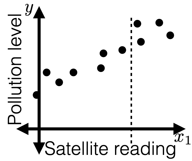
Recall
- A general ML approach
- Collect data
- Choose hypothesis class, hyperparameter, loss function
- Train (optimize for) "good" hypothesis by minimizing loss.


- Limitations of a closed-form solution for objective minimizer
- Don't always have closed-form solutions. (Recall, half-pipe cases.)
- Ridge came to the rescue, but we don't always have such "savior".
- Even when closed-form solutions exist, can be expensive to compute (recall, lab2, Q2.8)
- Want a more general, efficient way! (=> GD methods today)
Outline
- Recap, motivation for gradient descent methods
-
Gradient descent algorithm (GD)
- The gradient vector
- GD algorithm
- Gradient decent properties
- convex functions, local vs global min
- Stochastic gradient descent (SGD)
- SGD algorithm and setup
- GD vs SGD comparison
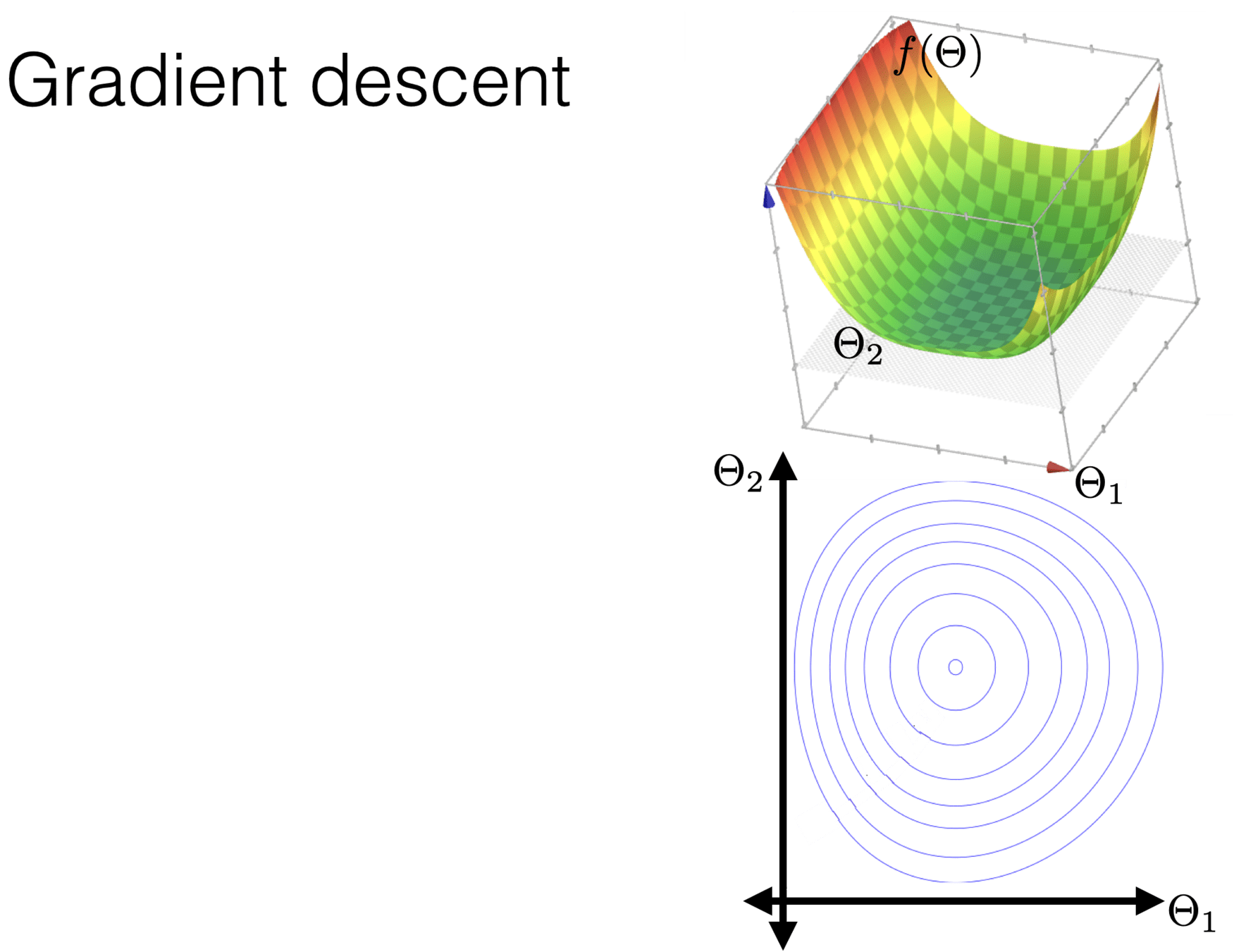
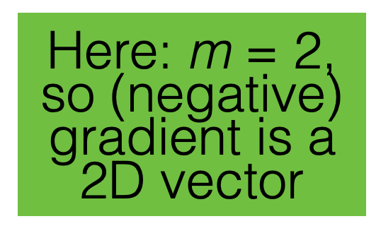
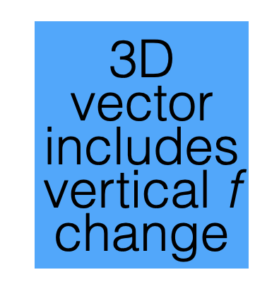
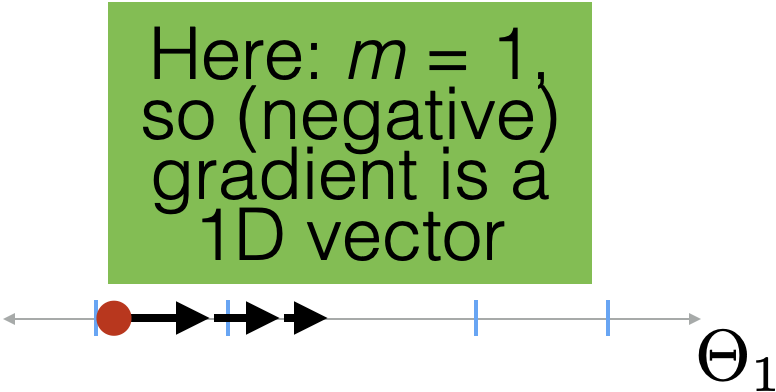
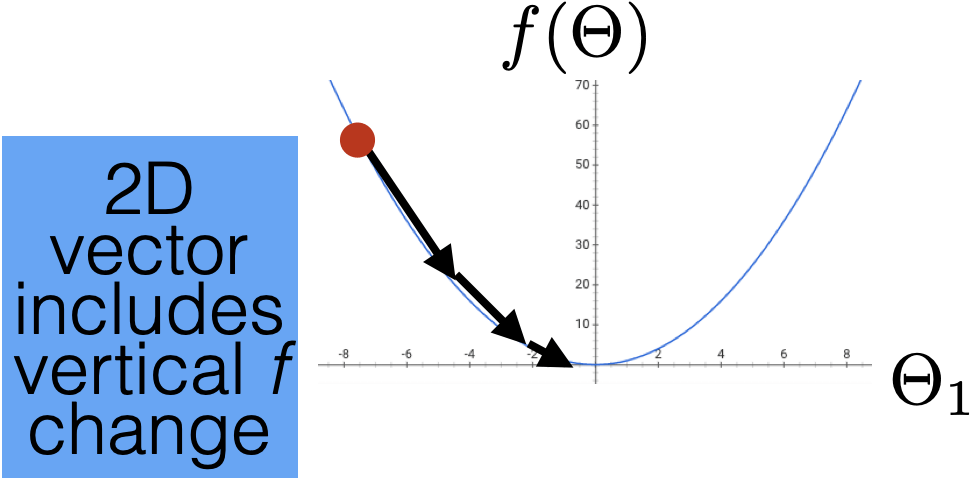
For \(f: \mathbb{R}^m \rightarrow \mathbb{R}\), its gradient \(\nabla f: \mathbb{R}^m \rightarrow \mathbb{R}^m\) is defined at the point \(p=\left(x_1, \ldots, x_m\right)\) in \(m\)-dimensional space as the vector
- Generalizes 1-dimensional derivatives.
- By construction, always has the same dimensionality as the function input.
(Aside: sometimes, the gradient doesn't exist, or doesn't behave nicely, as we'll see later in this course. For today, we have well-defined, nice, gradients.)
Gradient
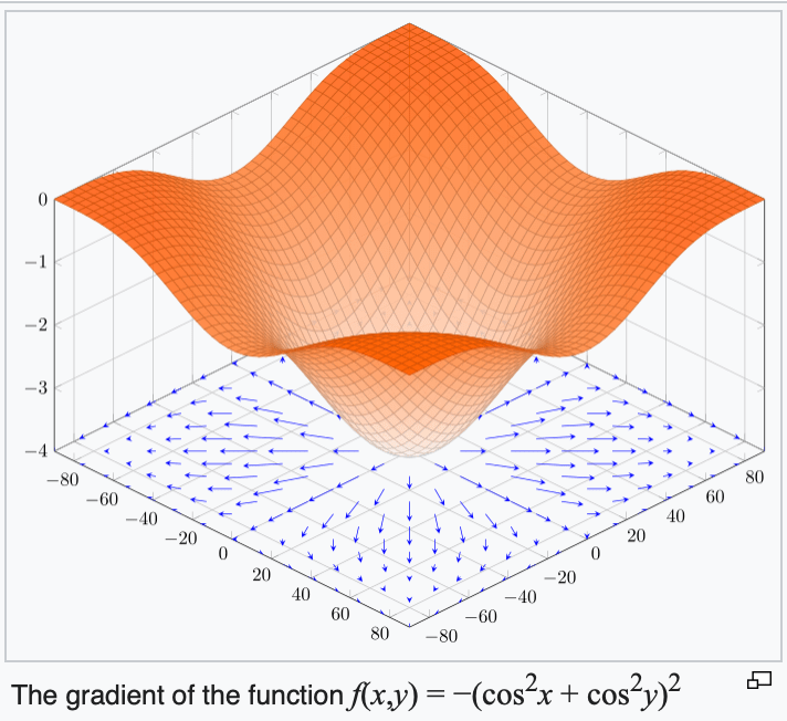
another example
a gradient can be the (symbolic) function
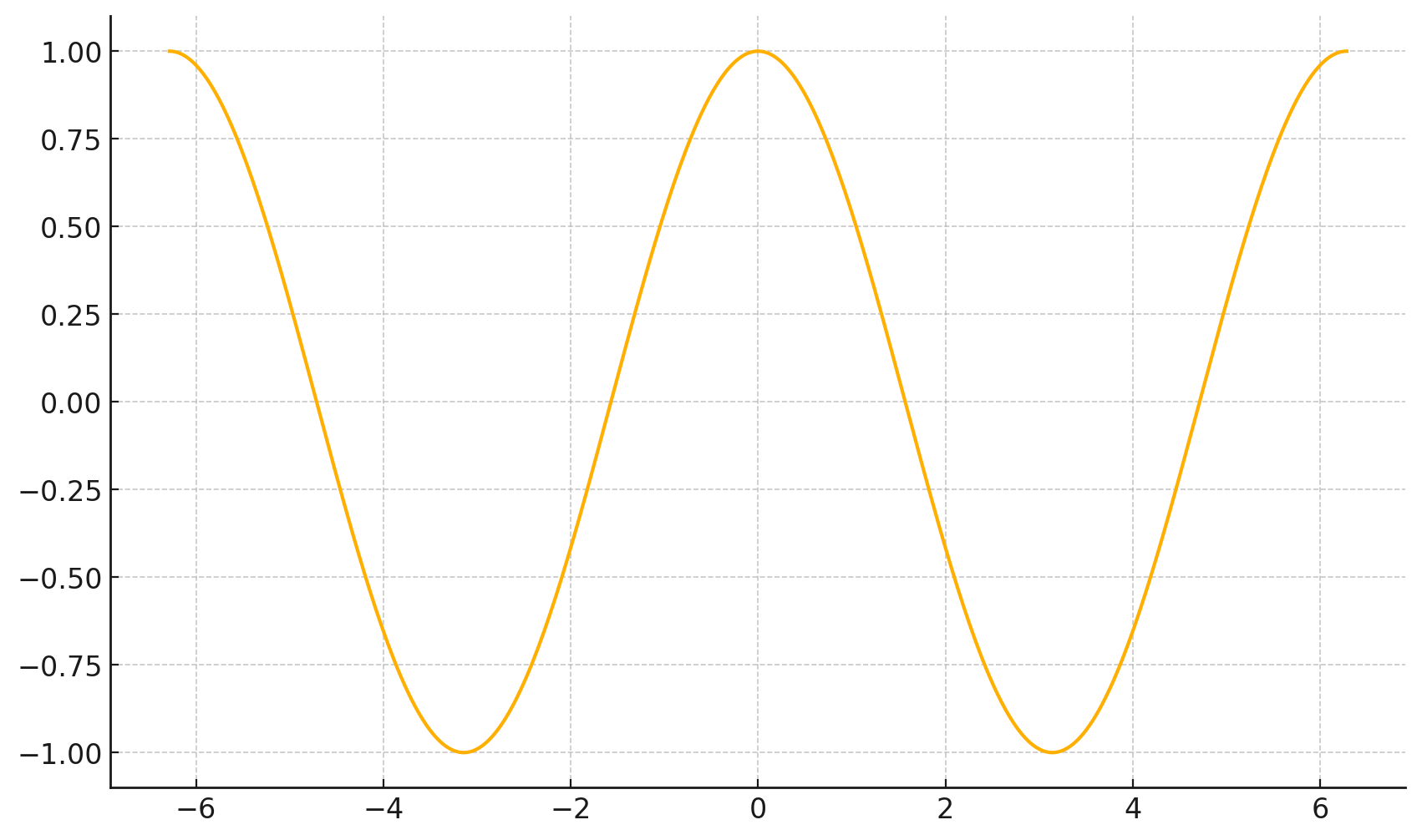
one cute example:
exactly like how derivative can be both a function and a number.
or,
we can also evaluate the gradient function at a point and get (numerical) gradient vectors
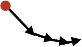
3. the gradient points in the direction of the (steepest) increase in the function value.
\(\frac{d}{dx} \cos(x) \bigg|_{x = -4} = -\sin(-4) \approx -0.7568\)
\(\frac{d}{dx} \cos(x) \bigg|_{x = 5} = -\sin(5) \approx 0.9589\)
Outline
- Recap, motivation for gradient descent methods
-
Gradient descent algorithm (GD)
- The gradient vector
- GD algorithm
- Gradient decent properties
- convex functions, local vs global min
- Stochastic gradient descent (SGD)
- SGD algorithm and setup
- GD vs SGD comparison
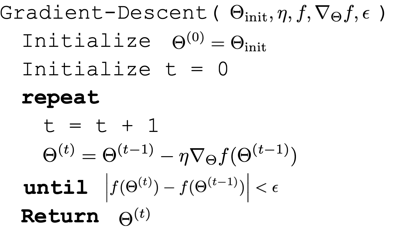
hyperparameters
initial guess
of parameters
learning rate,
aka, step size
precision
1
2
3
4
5
6
7
8


1
2
3
4
5
6
7
8

1
2
3
4
5
6
7
8
1
2
3
4
5
6
7
8
1
2
3
4
5
6
7
8
1
2
3
4
5
6
7
8
1
2
3
4
5
6
7
8

1
2
3
4
5
6
7
8
Q: if this condition is satisfied, what does it imply?
A: the gradient at the current parameter is almost zero.
1
2
3
4
5
6
7
8
Other possible stopping criteria for line 7:
- Parameter norm change between iteration\(\left\|\Theta^{(t)}-\Theta^{(t-1)}\right\|<\epsilon\)
- Gradient norm close to zero \(\left\|\nabla_{\Theta} f\left(\Theta^{(t)}\right)\right\|<\epsilon\)
- Max number of iterations \(T\)
1
2
3
4
5
6
7
8
Outline
- Recap, motivation for gradient descent methods
-
Gradient descent algorithm (GD)
- The gradient vector
- GD algorithm
-
Gradient decent properties
- convex functions, local vs global min
- Stochastic gradient descent (SGD)
- SGD algorithm and setup
- GD vs SGD comparison

When minimizing a function, we'd hope to get to a global minimizer
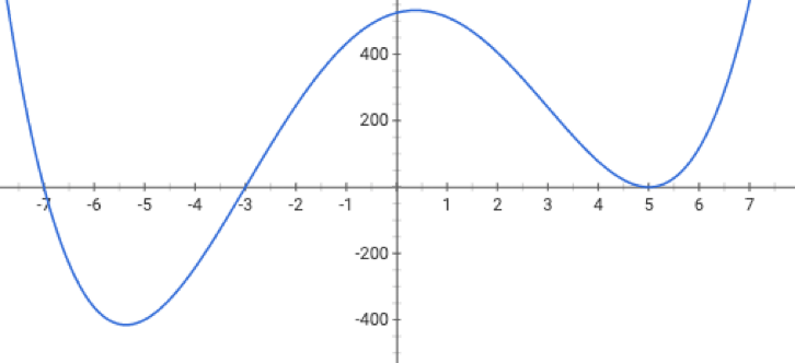


At a global minimizer
the gradient vector is the zero vector
\(\Rightarrow\)
\(\nLeftarrow\)

When minimizing a function, we'd hope to get to a global minimizer
At a global minimizer
the gradient vector is the zero vector
\(\Leftarrow\)
the function is a convex function
A function \(f\) is convex
if any line segment connecting two points of the graph of \(f\) lies above or on the graph.
- (\(f\) is concave if \(-f\) is convex.)
- (one can say a lot about optimization convergence for convex functions.)
Some examples
Convex functions
Non-convex functions


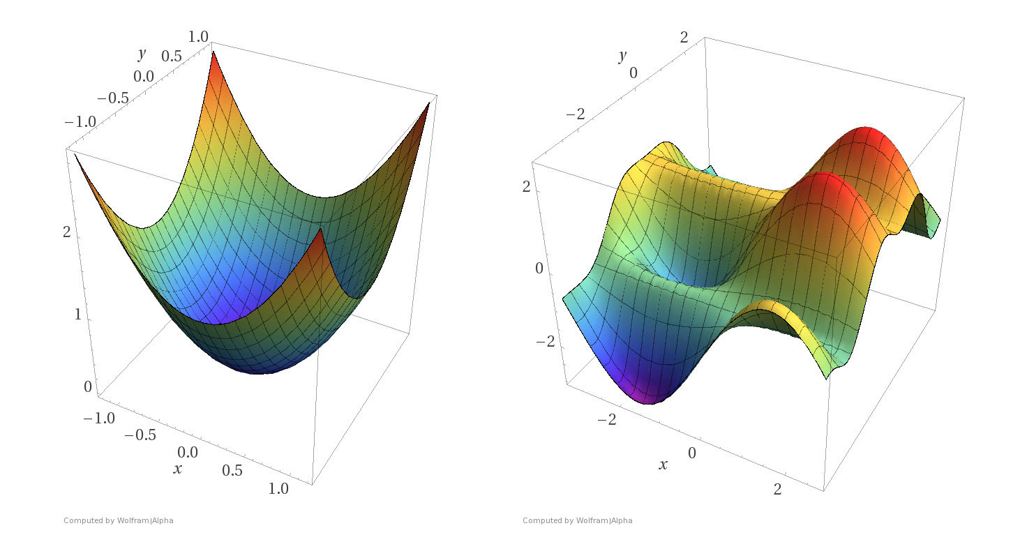


- A function \(f\) on \(\mathbb{R}^m\) is convex if any line segment connecting two points of the graph of \(f\) lies above or on the graph.
- For convex functions, all local minima are global minima.
What do we need to know:
- Intuitive understanding of the definition
- If given a function, can determine if it's convex. (We'll only ever give at most 2D, so visual understanding is enough)
- Understand how gradient descent algorithms may "fail" without convexity.
- Recognize that OLS loss function is convex, ridge regression loss is (strictly) convex, and later cross-entropy loss function is convex too.
- Assumptions:
- \(f\) is sufficiently "smooth"
- \(f\) has at least one global minimum
- Run the algorithm long enough
- \(\eta\) is sufficiently small
- \(f\) is convex
- Conclusion:
- Gradient descent will return a parameter value within \(\tilde{\epsilon}\) of a global minimum (for any chosen \(\tilde{\epsilon}>0\) )
Gradient Descent Performance
if violated, may not have gradient,
can't run gradient descent
- Assumptions:
- \(f\) is sufficiently "smooth"
- \(f\) has at least one global minimum
- Run the algorithm long enough
- \(\eta\) is sufficiently small
- \(f\) is convex
- Conclusion:
- Gradient descent will return a parameter value within \(\tilde{\epsilon}\) of a global minimum (for any chosen \(\tilde{\epsilon}>0\) )
Gradient Descent Performance
if violated:
may not terminate/no minimum to converge to

- Assumptions:
- \(f\) is sufficiently "smooth"
- \(f\) has at least one global minimum
- Run the algorithm long enough
- \(\eta\) is sufficiently small
- \(f\) is convex
- Conclusion:
- Gradient descent will return a parameter value within \(\tilde{\epsilon}\) of a global minimum (for any chosen \(\tilde{\epsilon}>0\)
Gradient Descent Performance
if violated:
see demo on next slide, also lab/recitation/hw
- Assumptions:
- \(f\) is sufficiently "smooth"
- \(f\) has at least one global minimum
- Run the algorithm long enough
- \(\eta\) is sufficiently small
- \(f\) is convex
- Conclusion:
- Gradient descent will return a parameter value within \(\tilde{\epsilon}\) of a global minimum (for any chosen \(\tilde{\epsilon}>0\) )
Gradient Descent Performance
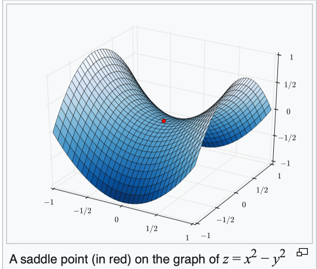
if violated, may get stuck at a saddle point
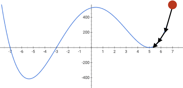
or a local minimum
Gradient descent performance
- Assumptions:
- \(f\) is sufficiently "smooth"
- \(f\) has at least one global minimum
- Run the algorithm sufficiently "long"
- \(\eta\) is sufficiently small
- \(f\) is convex
- Conclusion:
- Gradient descent will return a parameter value within \(\tilde{\epsilon}\) of a global minimum (for any chosen \(\tilde{\epsilon}>0\) )
Outline
- Recap, motivation for gradient descent methods
- Gradient descent algorithm (GD)
- The gradient vector
- GD algorithm
- Gradient decent properties
- convex functions, local vs global min
-
Stochastic gradient descent (SGD)
- SGD algorithm and setup
- GD vs SGD comparison
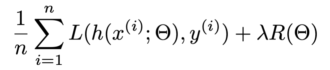
Gradient of an ML objective
- An ML objective function is a finite sum
- the MSE of a linear hypothesis:
- The gradient of an ML objective :
- and its gradient w.r.t. \(\theta\):
In general,
For instance,
(gradient of the sum) = (sum of the gradient)
👆
Concrete example
Three data points:
{(2,5), (3,6), (4,7)}
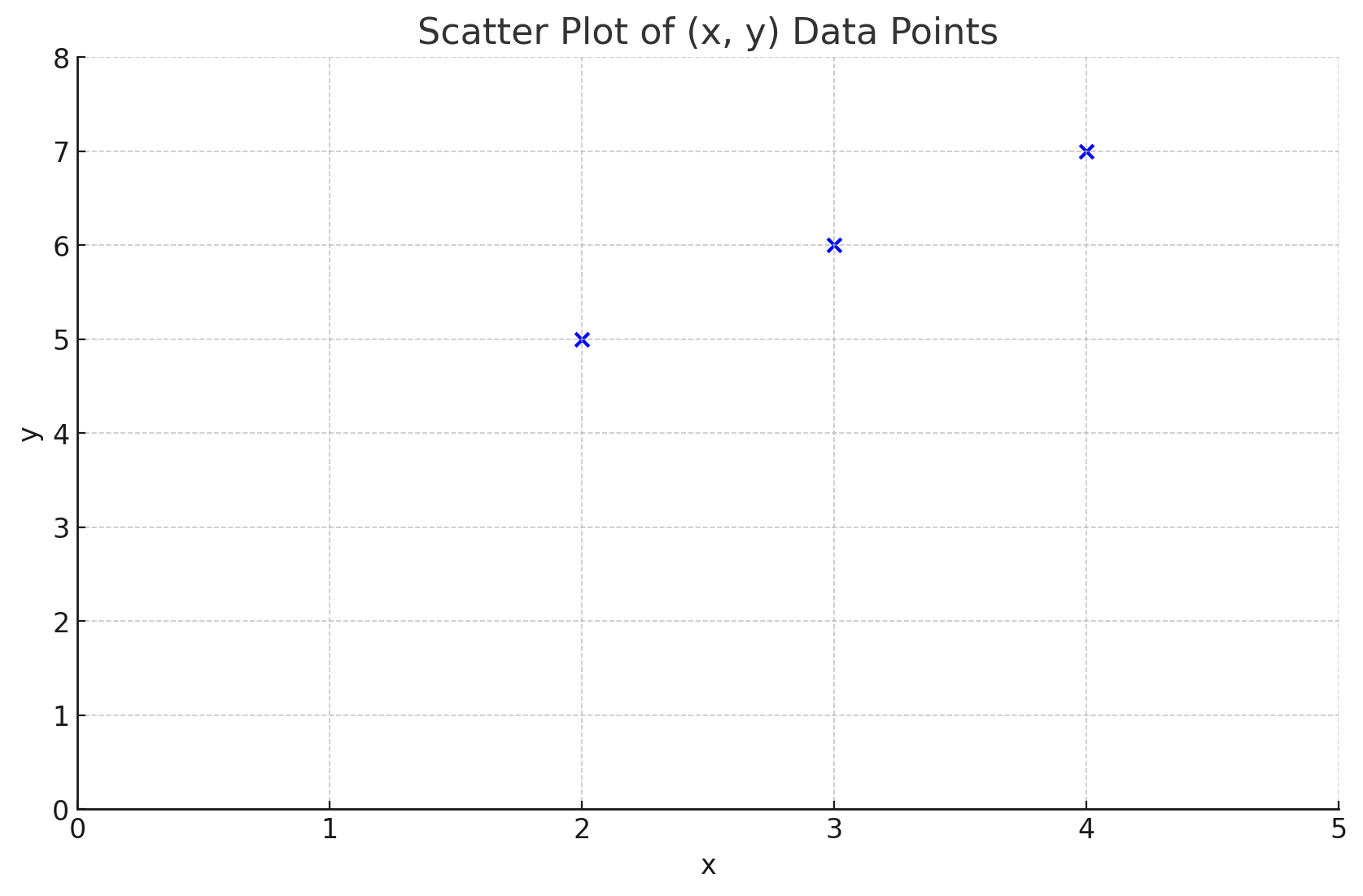
Fit a line (without offset) to the dataset, MSE:
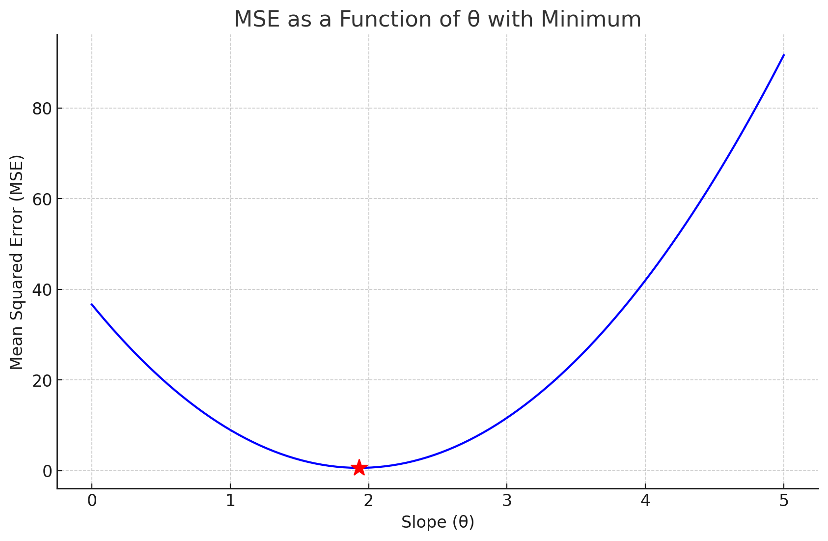
First data point's "pull"
Second data point 's "pull"
Third data point's "pull"
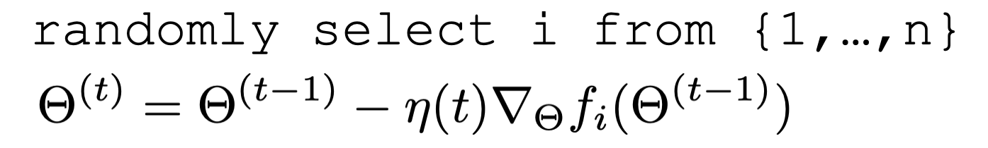
Stochastic gradient descent
for a randomly picked data point \(i\)

- Assumptions:
- \(f\) is sufficiently "smooth"
- \(f\) has at least one global minimum
- Run the algorithm long enough
- \(\eta\) is sufficiently small and satisfies additional "scheduling" condition
- \(f\) is convex
- Conclusion:
- Stochastic gradient descent will return a parameter value within \(\tilde{\epsilon}\) of a global minimum with probability 1 (for any chosen \(\tilde{\epsilon}>0\) )
Stochastic gradient descent performance
\(\sum_{t=1}^{\infty} \eta(t)=\infty\) and \(\sum_{t=1}^{\infty} \eta(t)^2<\infty\)
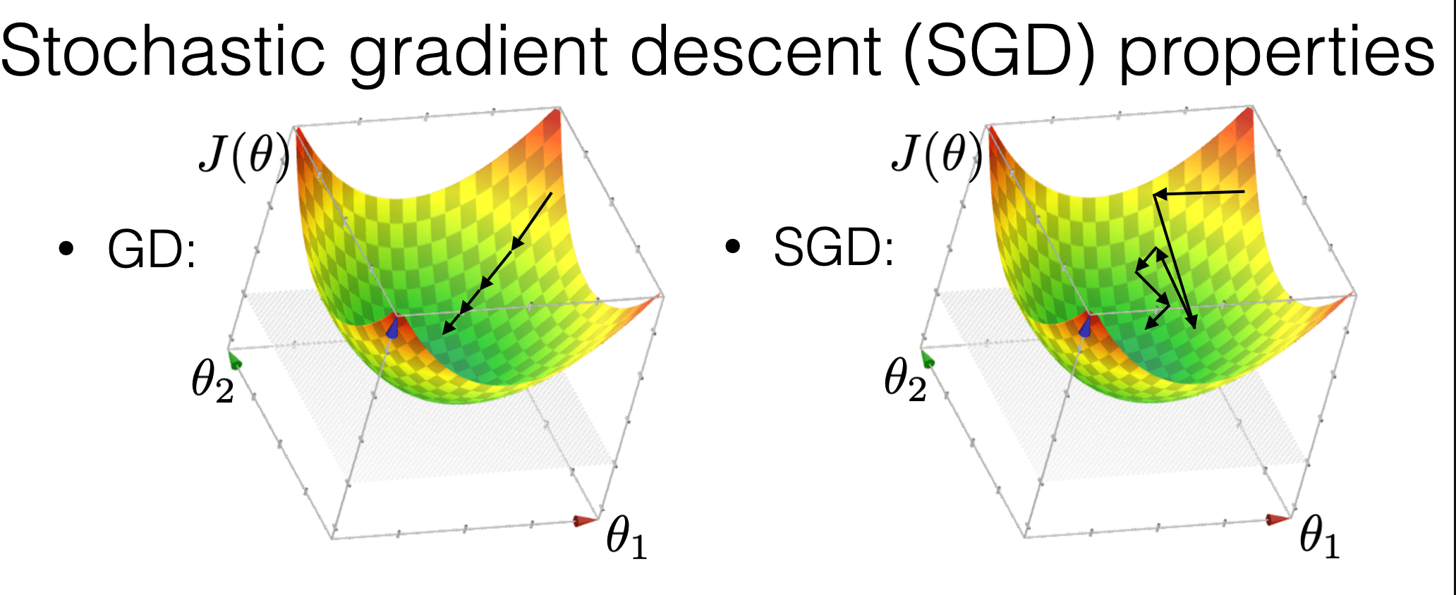
is more "random"
is more efficient
may get us out of a local min

Compared with GD, SGD
Summary
-
Most ML methods can be formulated as optimization problems.
-
We won’t always be able to solve optimization problems analytically (in closed-form).
-
We won’t always be able to solve (for a global optimum) efficiently.
-
We can still use numerical algorithms to good effect. Lots of sophisticated ones available.
-
Introduce the idea of gradient descent in 1D: only two directions! But magnitude of step is important.
-
In higher dimensions the direction is very important as well as magnitude.
-
GD, under appropriate conditions (most notably, when objective function is convex), can guarantee convergence to a global minimum.
-
SGD: approximated GD, more efficient, more random, and less guarantees.
Thanks!
We'd love to hear your thoughts.