

Lecture 6: Neural Networks
Shen Shen
Oct 4, 2024
Intro to Machine Learning

Outline
- Recap, the leap from simple linear models
- (Feedforward) Neural Networks Structure
- Design choices
- Forward pass
- Backward pass
- Back-propagation
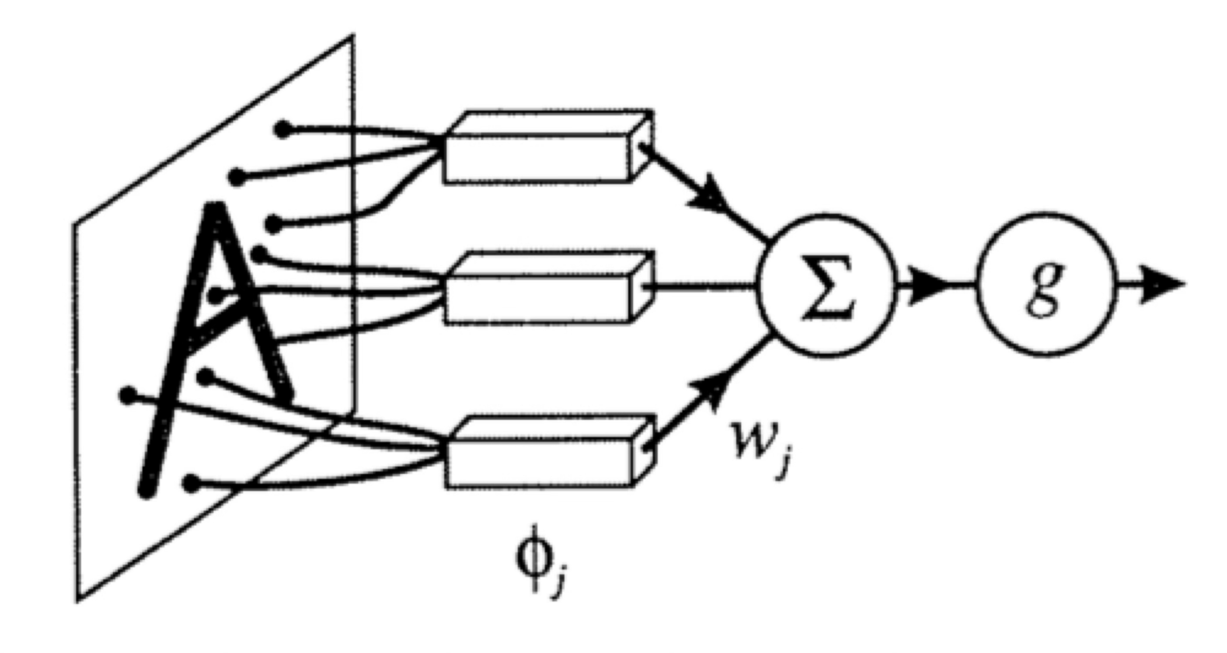
Recap:
leveraging nonlinear transformations
👆
importantly, linear in \(\phi\), non-linear in \(x\)
transform via

Pointed out key ideas (enabling neural networks):
- Nonlinear feature transformation
- "Composing" simple transformations
- Backpropagation
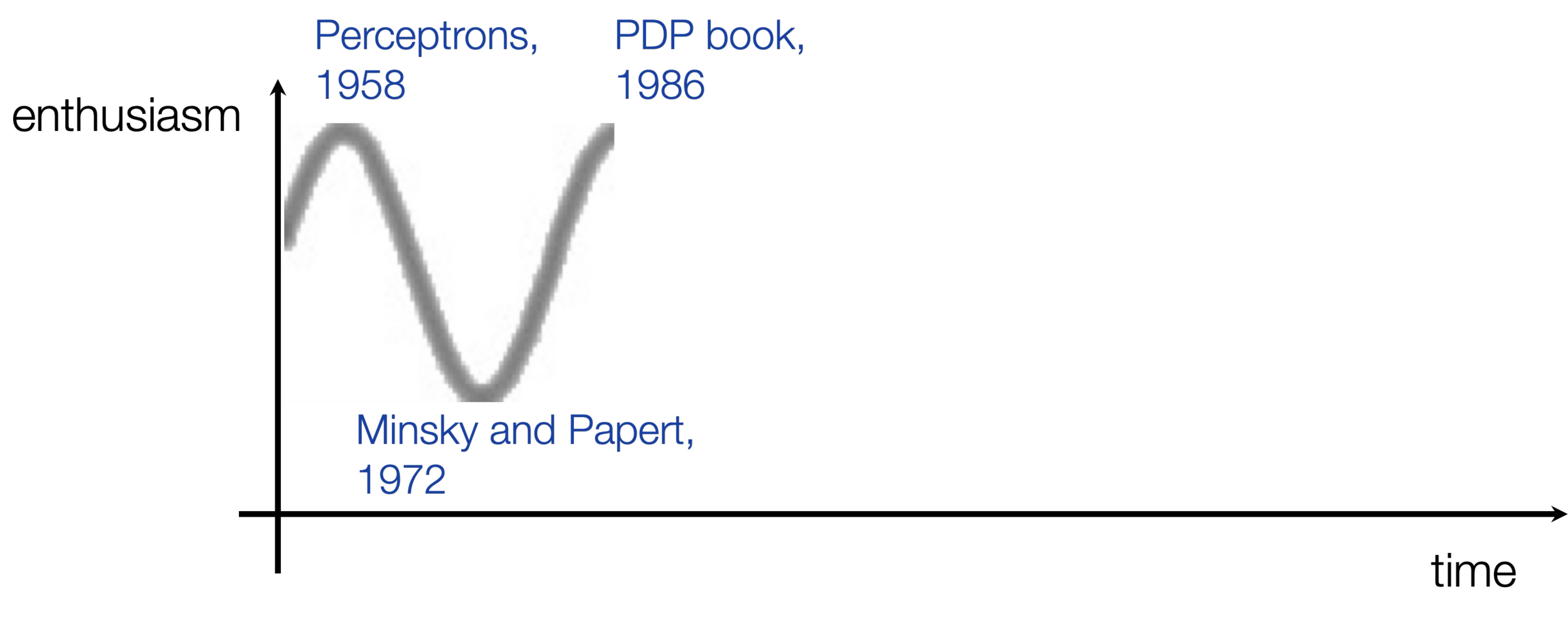
expressiveness
efficient training
Two epiphanies:
- nonlinear transformation empowers linear tools
- "composing" simple nonlinearities amplifies such effect
some appropriate weighted sum
Outline
- Recap, the leap from simple linear models
-
(Feedforward) Neural Networks Structure
- Design choices
- Forward pass
- Backward pass
- Back-propagation
👋 heads-up, in this section, for simplicity:
all neural network diagrams focus on a single data point
A neuron:
\(w\): what the algorithm learns
- \(x\): \(d\)-dimensional input
A neuron:
- \(a\): post-activation output
- \(f\): activation function
- \(w\): weights (i.e. parameters)
- \(z\): pre-activation output
\(f\): what we engineers choose
\(z\): scalar
\(a\): scalar
Choose activation \(f(z)=z\)
learnable parameters (weights)
e.g. linear regressor represented as a computation graph
Choose activation \(f(z)=\sigma(z)\)
learnable parameters (weights)
e.g. linear logistic classifier represented as a computation graph
A layer:
learnable weights
A layer:
- (# of neurons) = (layer's output dimension).
- typically, all neurons in one layer use the same activation \(f\) (if not, uglier algebra).
- typically fully connected, where all \(x_i\) are connected to all \(z_j,\) meaning each \(x_i\) influences every \(a_j\) eventually.
- typically, no "cross-wiring", meaning e.g. \(z_1\) won't affect \(a^2.\) (the final layer may be an exception if softmax is used.)
layer
linear combo
activations
A (fully-connected, feed-forward) neural network:
layer
input
neuron
learnable weights
We choose:
- activation \(f\) in each layer
- # of layers
- # of neurons in each layer
hidden
output
Outline
- Recap, the leap from simple linear models
- (Feedforward) Neural Networks Structure
- Design choices
- Forward pass
- Backward pass
- Back-propagation
some appropriate weighted sum
recall this example
\(f(\cdot) = \sigma(\cdot)\)
\(f(\cdot) \) identity function
it can be represented as
Activation function \(f\) choices
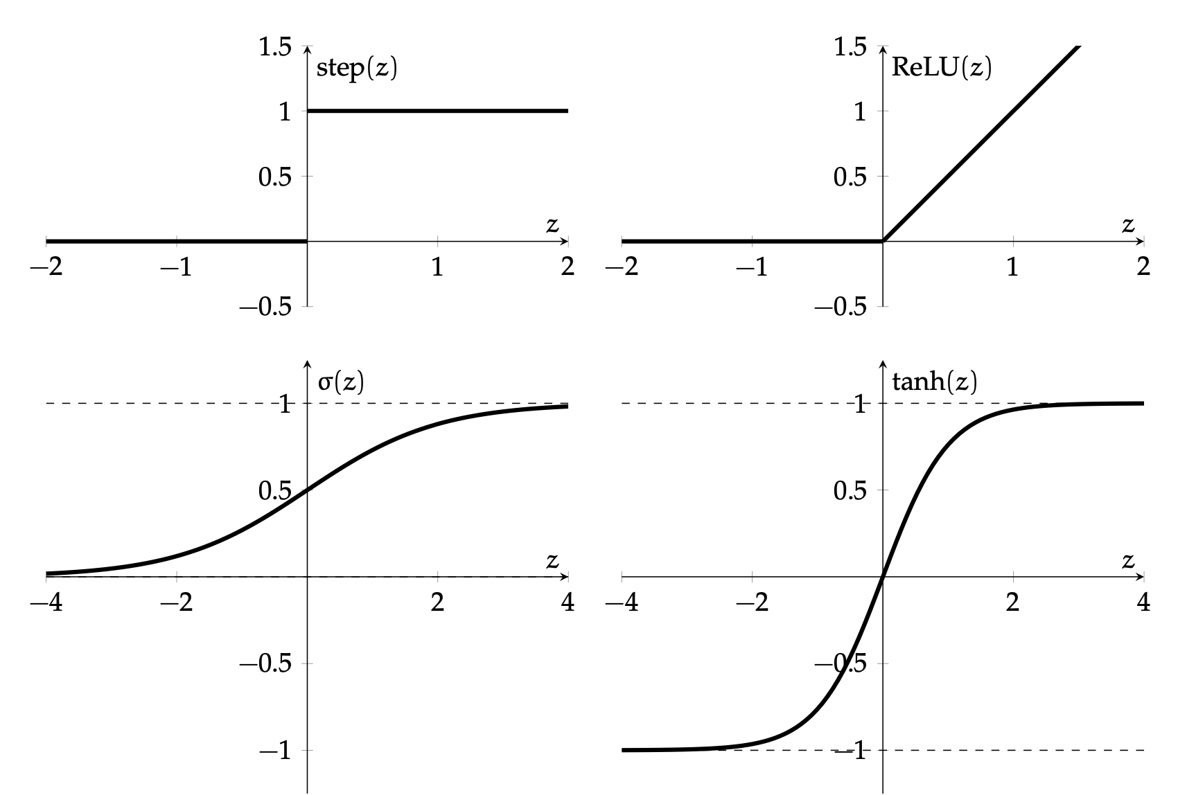
\(\sigma\) used to be the most popular
- firing rate of a neuron
- elegant gradient \(\sigma^{\prime}(z)=\sigma(z) \cdot(1-\sigma(z))\)
- default choice in hidden layers
- very simple function form, so is the gradient.
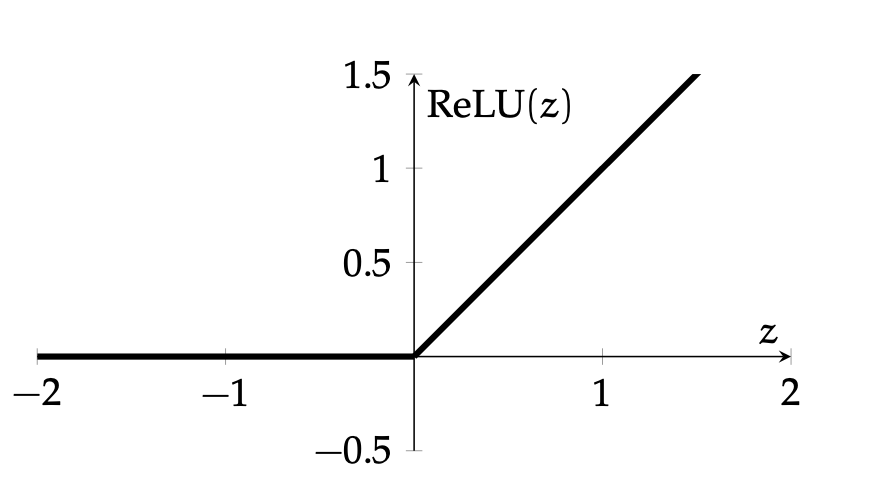
nowadays
- drawback: if strongly in negative region, a single ReLU can be "dead" (no gradient).
- Luckily, typically we have lots of units, so not everyone is dead.
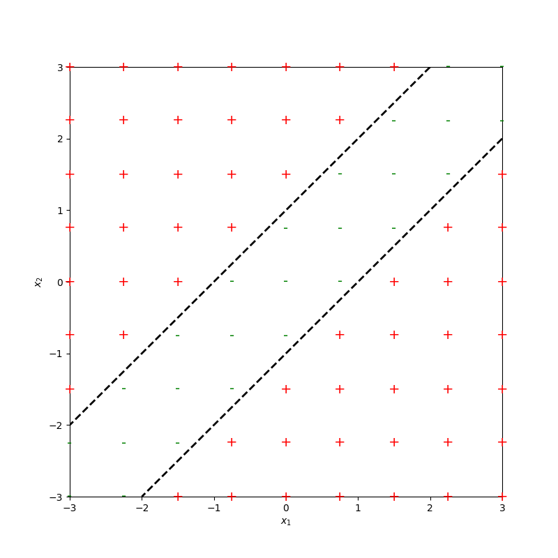
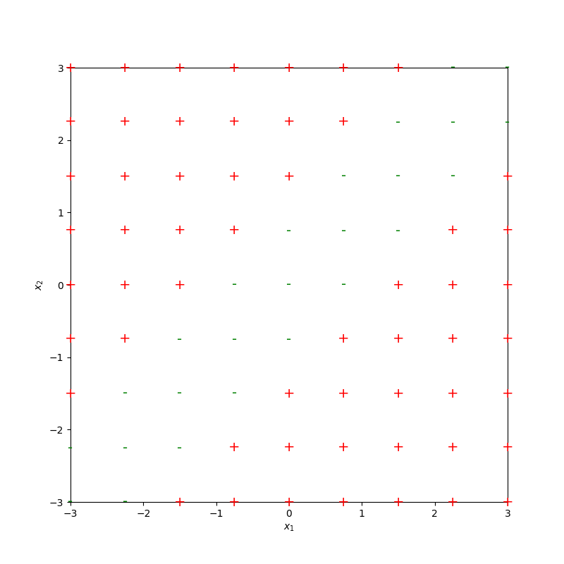
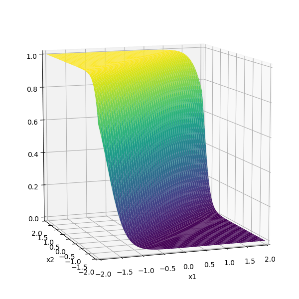
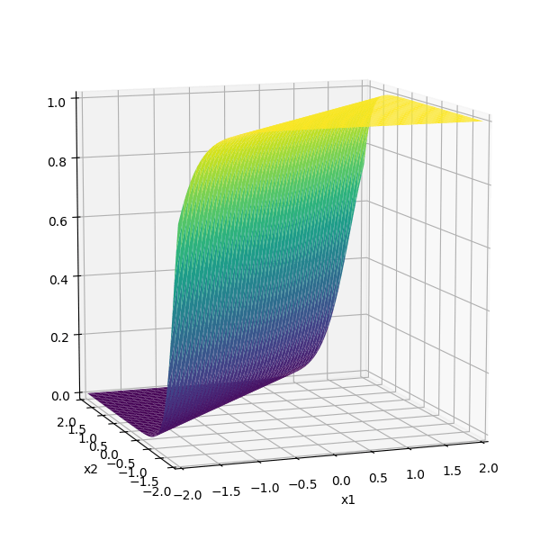
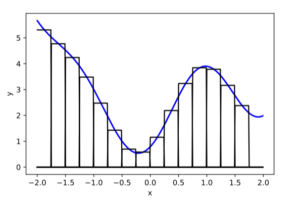
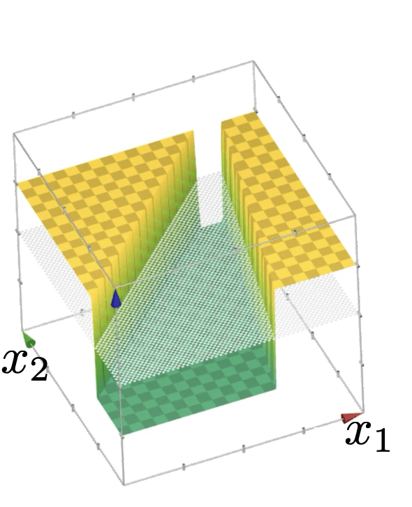
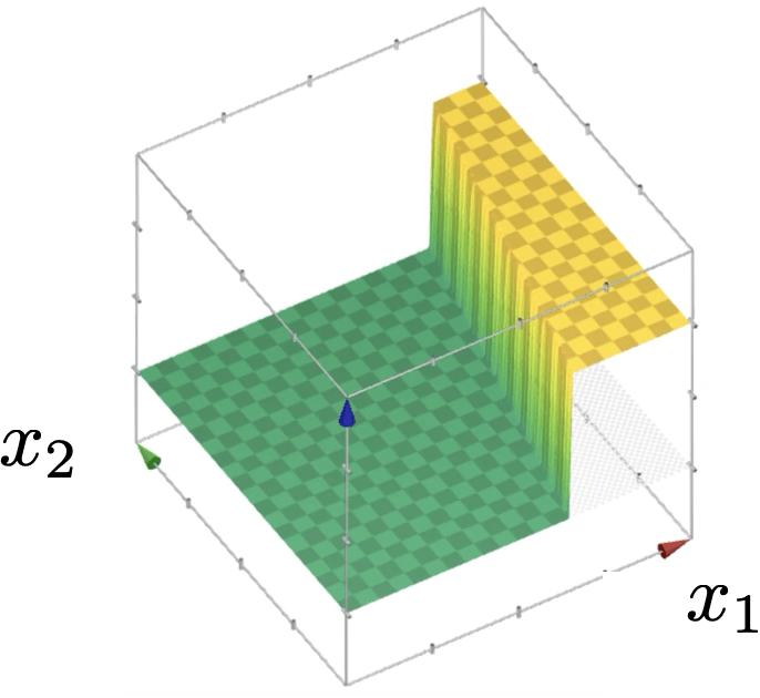
compositions of ReLU(s) can be quite expressive
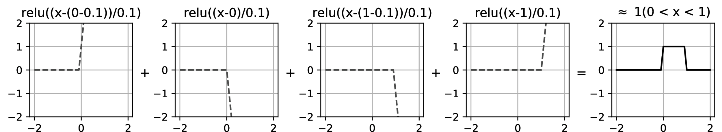
in fact, asymptotically, can approximate any function!
(image credit: Phillip Isola)
(image credit: Tamara Broderick)
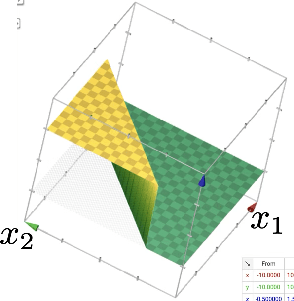
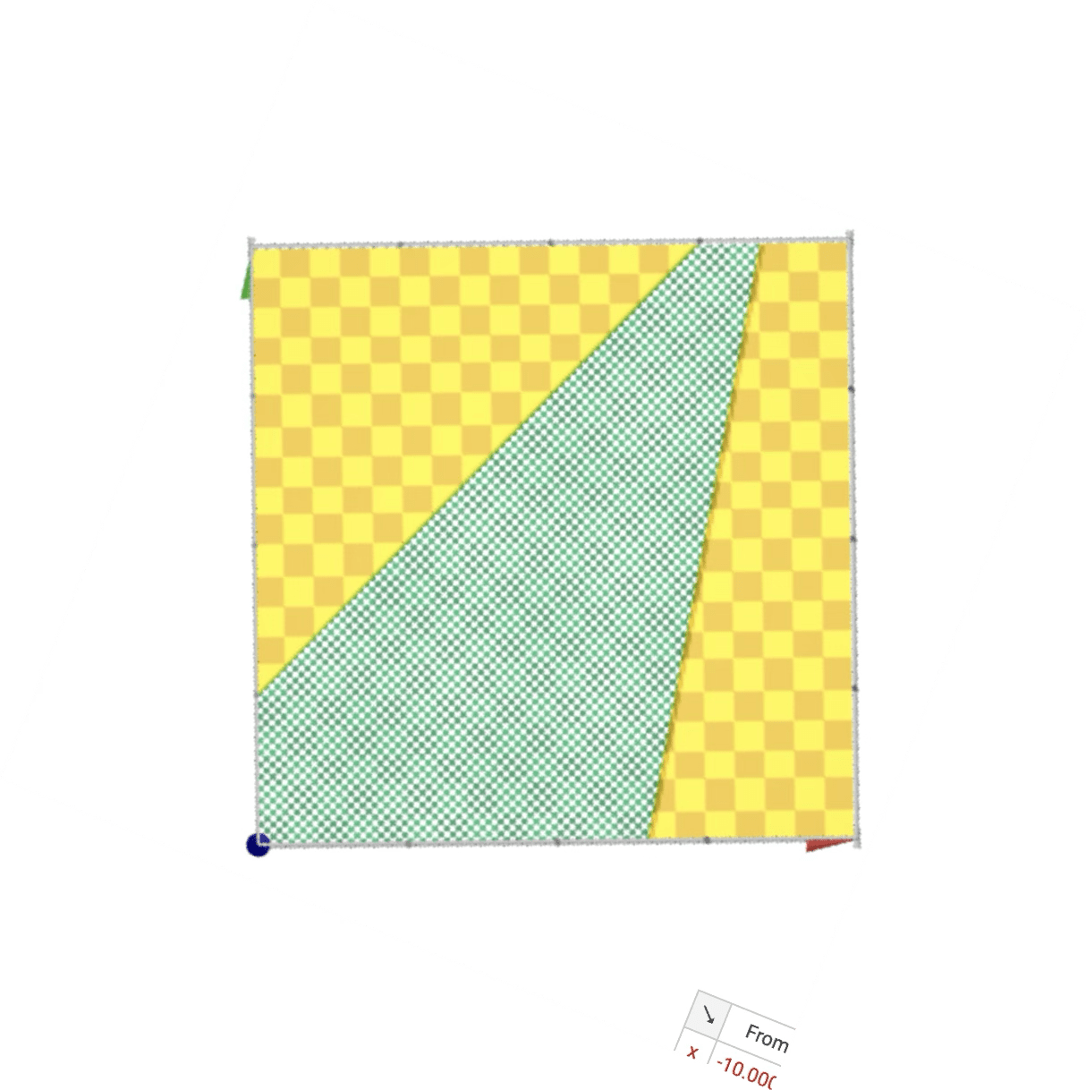
or give arbitrary decision boundaries!

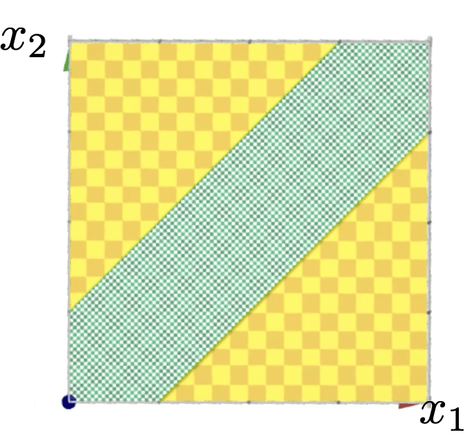
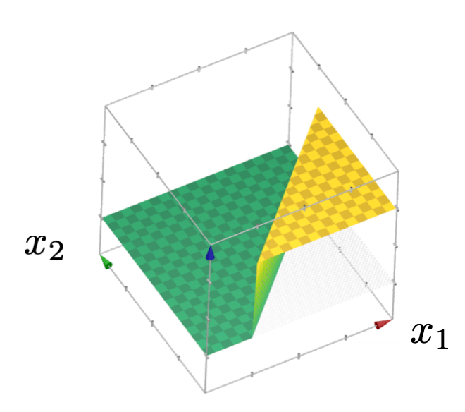
(image credit: Tamara Broderick)
output layer design choices
- # neurons, activation, and loss depend on the high-level goal.
- typically straightforward.
- Multi-class setup: if predict one and only one class out of \(K\) possibilities, then last layer: \(K\) neurons, softmax activation, cross-entropy loss
- other multi-class settings, see discussion in lab.
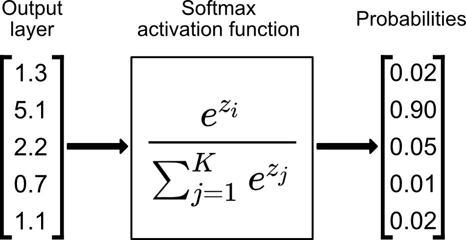
e.g., say \(K=5\) classes
input \(x\)
hidden layer(s)
output layer

- Width: # of neurons in layers
- Depth: # of layers
- More expressive if increasing either the width or depth.
- The usual pitfall of overfitting (though in NN-land, it's also an active research topic.)
(The demo won't embed in PDF. But the direct link below works.)
Outline
- Recap, the leap from simple linear models
- (Feedforward) Neural Networks Structure
- Design choices
- Forward pass
- Backward pass
- Back-propagation
- Evaluate the loss \(\mathcal{L} = (g-y)^2\)
- Repeat for each data point, average the sum of \(n\) individual losses
e.g. forward-pass of a linear regressor
- Evaluate the loss \(\mathcal{L} = - [y \log g+\left(1-y\right) \log \left(1-g\right)]\)
- Repeat for each data point, average the sum of \(n\) individual losses
e.g. forward-pass of a linear logistic classifier
linear combination
nonlinear activation
\(\dots\)
Forward pass:
evaluate, given the current parameters,
- the model output \(g^{(i)}\) =
- the loss incurred on the current data \(\mathcal{L}(g^{(i)}, y^{(i)})\)
- the training error \(J = \frac{1}{n} \sum_{i=1}^{n}\mathcal{L}(g^{(i)}, y^{(i)})\)
loss function
Outline
- Recap, the leap from simple linear models
- (Feedforward) Neural Networks Structure
- Design choices
- Forward pass
-
Backward pass
- Back-propagation
- Randomly pick a data point \((x^{(i)}, y^{(i)})\)
- Evaluate the gradient \(\nabla_{W^2} \mathcal{L(g^{(i)},y^{(i)})}\)
- Update the weights \(W^2 \leftarrow W^2 - \eta \nabla_{W^2} \mathcal{L(g^{(i)},y^{(i)}})\)
\(\dots\)
Backward pass:
Run SGD to update the parameters, e.g. to update \(W^2\)

\(\nabla_{W^2} \mathcal{L(g^{(i)},y^{(i)})}\)
\(\dots\)
\(\nabla_{W^2} \mathcal{L(g,y)}\)
Backward pass:
Run SGD to update the parameters, e.g. to update \(W^2\)
Evaluate the gradient \(\nabla_{W^2} \mathcal{L(g^{(i)},y^{(i)})}\)
Update the weights \(W^2 \leftarrow W^2 - \eta \nabla_{W^2} \mathcal{L(g^{(i)},y^{(i)}})\)
How do we get these gradient though?
\(\nabla_{W^1} \mathcal{L(g,y)}\)
Backward pass:
Run SGD to update the parameters, e.g. to update \(W^1\)
Evaluate the gradient \(\nabla_{W^1} \mathcal{L(g^{(i)},y^{(i)})}\)
Update the weights \(W^1 \leftarrow W^1 - \eta \nabla_{W^1} \mathcal{L(g^{(i)},y^{(i)}})\)
\(\dots\)
Outline
- Recap, the leap from simple linear models
- (Feedforward) Neural Networks Structure
- Design choices
- Forward pass
-
Backward pass
- Back-propagation
e.g. backward-pass of a linear regressor
- Randomly pick a data point \((x^{(i)}, y^{(i)})\)
- Evaluate the gradient \(\nabla_{w} \mathcal{L(g^{(i)},y^{(i)})}\)
- Update the weights \(w \leftarrow w - \eta \nabla_w \mathcal{L(g^{(i)},y^{(i)}})\)
e.g. backward-pass of a linear regressor
e.g. backward-pass of a non-linear regressor
\(\dots\)
Now, back propagation: reuse of computation
how to find
?
\(\dots\)
back propagation: reuse of computation
how to find
?
\(\dots\)
back propagation: reuse of computation
how to find
?
Summary
- We saw that introducing non-linear transformations of the inputs can substantially increase the power of linear tools. But it’s kind of difficult/tedious to select a good transformation by hand.
- Multi-layer neural networks are a way to automatically find good transformations for us!
- Standard NNs have layers that alternate between parametrized linear transformations and fixed non-linear transforms (but many other designs are possible.)
- Typical non-linearities include sigmoid, tanh, relu, but mostly people use relu.
- Typical output transformations for classification are as we've seen: sigmoid, or softmax.
- There’s a systematic way to compute gradients via back-propagation, in order to update parameters.
Thanks!
We'd love to hear your thoughts.