x^{(1)}

y^{(1)}

f^1

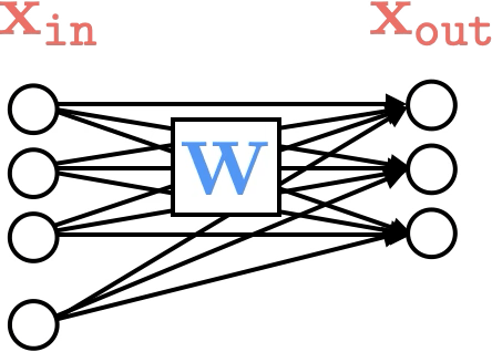
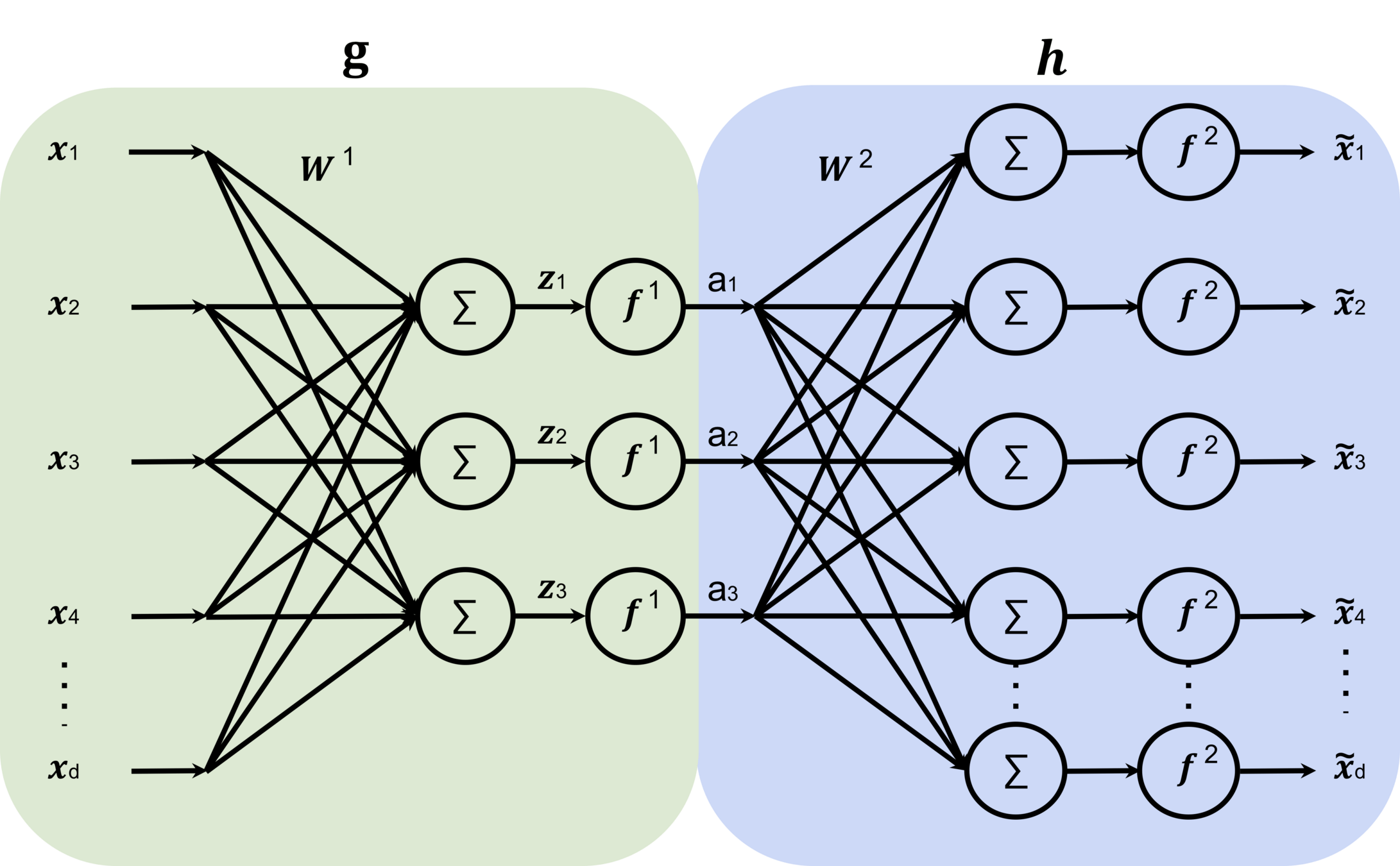
linear combination

nonlinear activation

\begin{aligned} & W^1 \\ \end{aligned}

\begin{aligned} & W^2 \\ \end{aligned}

\begin{aligned} & W^L \\ \end{aligned}

f^2

f^L

g^{(1)}

\(\dots\)

f^2\left(\hspace{2cm}; \mathbf{W}^2\right)

f^1(\mathbf{x}^{(i)}; \mathbf{W}^1)

f^L\left(\dots \hspace{3.5cm}; \dots \mathbf{W}^L\right)

Forward pass: evaluate, given the current parameters,

the model output \(g^{(i)}\) =

the loss incurred on the current data \(\mathcal{L}(g^{(i)}, y^{(i)})\)

the training error \(J = \frac{1}{n} \sum_{i=1}^{n}\mathcal{L}(g^{(i)}, y^{(i)})\)

\mathcal{L}(g^{(1)}, y^{(1)})

\mathcal{L}(g, y)

\mathcal{L}(g^{(n)}, y^{(n)})

\underbrace{\quad \quad \quad \quad \quad } \\ n

\dots

loss function

Recap:

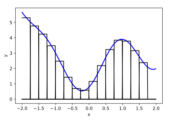
compositions of ReLU(s) can be quite expressive

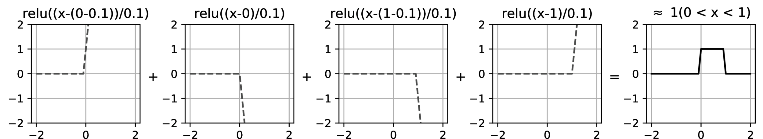
in fact, asymptotically, can approximate any function!

(image credit: Phillip Isola)

\sigma_1 = \sigma(5 x_1 + -5 x_2 + 1)

\sigma_2 = \sigma(-5 x_1 + 5 x_2 + 1)

some weighted sum

Recap:

Randomly pick a data point \((x^{(i)}, y^{(i)})\)
Evaluate the gradient \(\nabla_{W^2} \mathcal{L(g^{(i)},y^{(i)})}\)
Update the weights \(W^2 \leftarrow W^2 - \eta \nabla_{W^2} \mathcal{L(g^{(i)},y^{(i)}})\)

x^{(i)}

y^{(i)}

f^1

\begin{aligned} & W^1 \\ \end{aligned}

\begin{aligned} & W^2 \\ \end{aligned}

\begin{aligned} & W^L \\ \end{aligned}

f^2

f^L

g^{(i)}

\(\dots\)

\mathcal{L}(g^{(i)}, y^{(i)})

\mathcal{L}(g, y)

\mathcal{L}(g^{(n)}, y^{(n)})

\underbrace{\quad \quad \quad \quad \quad } \\ n

\dots

Backward pass: run SGD to update the parameters, e.g. to update \(W^2\)

\(\nabla_{W^2} \mathcal{L(g^{(i)},y^{(i)})}\)

Recap:

x

\(\dots\)

y

f^1

\begin{aligned} & W^1 \\ \end{aligned}

\begin{aligned} & W^2 \\ \end{aligned}

\begin{aligned} & W^L \\ \end{aligned}

f^2

f^L

\mathcal{L}(g,y)

g

Z^L

A^2

Z^2

A^1

Z^1

\frac{\partial \mathcal{L}(g,y)}{\partial g}

\frac{\partial g}{\partial Z^{L}}

\frac{\partial Z^3}{\partial A^{2}}\frac{\partial A^4}{\partial Z^{3}} \dots \frac{\partial Z^L}{\partial A^{L-1}}

\frac{\partial A^2}{\partial Z^{2}}

\frac{\partial \mathcal{L}(g,y)}{\partial Z^2}

\underbrace{\hspace{4cm}}

\underbrace{\hspace{4.7cm}}

\frac{\partial Z^2}{\partial W^{2}}

\frac{\partial \mathcal{L}(g,y)}{\partial W^2}

Recap:

back propagation: reuse of computation

\underbrace{\hspace{6.5cm}}

\frac{\partial Z^2}{\partial A^{1}}

\frac{\partial A^1}{\partial Z^{1}}

\frac{\partial Z^1}{\partial W^{1}}

x

\(\dots\)

y

f^1

\begin{aligned} & W^1 \\ \end{aligned}

\begin{aligned} & W^2 \\ \end{aligned}

\begin{aligned} & W^L \\ \end{aligned}

f^2

f^L

\mathcal{L}(g,y)

g

Z^L

A^2

Z^2

A^1

Z^1

\frac{\partial \mathcal{L}(g,y)}{\partial g}

\frac{\partial g}{\partial Z^{L}}

\frac{\partial Z^3}{\partial A^{2}}\frac{\partial A^4}{\partial Z^{3}} \dots \frac{\partial Z^L}{\partial A^{L-1}}

\frac{\partial A^2}{\partial Z^{2}}

\frac{\partial \mathcal{L}(g,y)}{\partial Z^2}

\underbrace{\hspace{4cm}}

\frac{\partial \mathcal{L}(g,y)}{\partial W^1}

\underbrace{\hspace{4.7cm}}

\frac{\partial Z^2}{\partial W^{2}}

\frac{\partial \mathcal{L}(g,y)}{\partial W^2}

back propagation: reuse of computation

Recap:

Outline

Recap, neural networks mechanism
Neural networks are representation learners
Auto-encoder:
- Bottleneck
- Reconstruction
Unsupervised learning
(Some recent representation learning ideas)

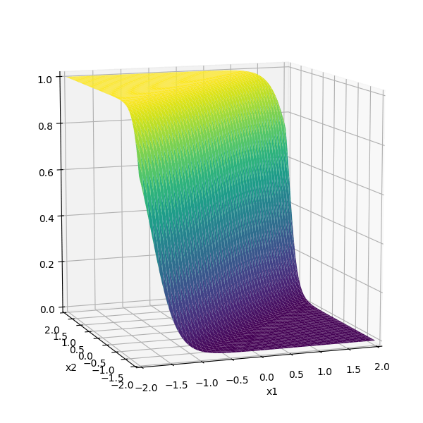
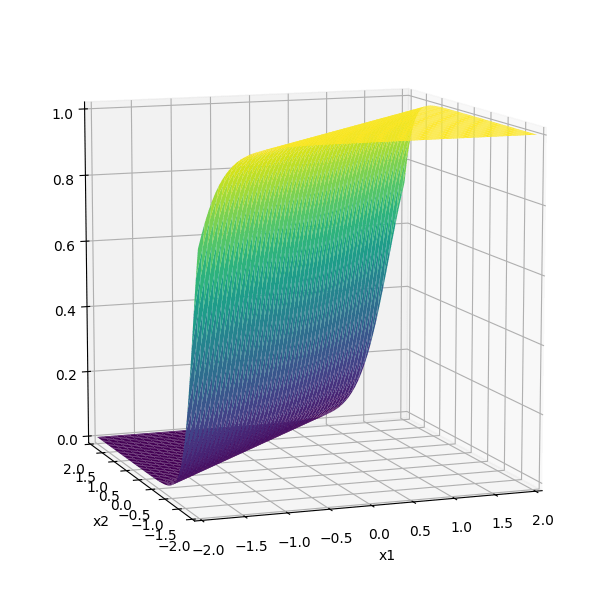
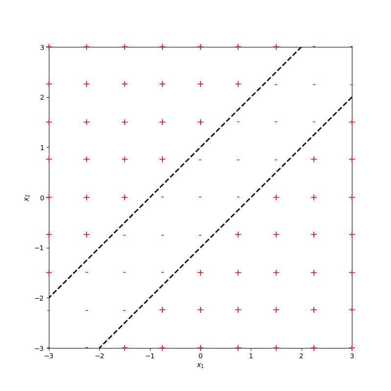
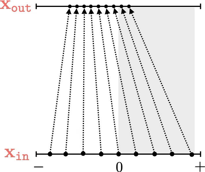
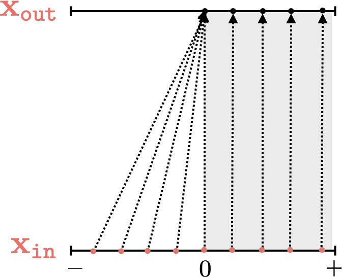
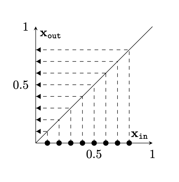
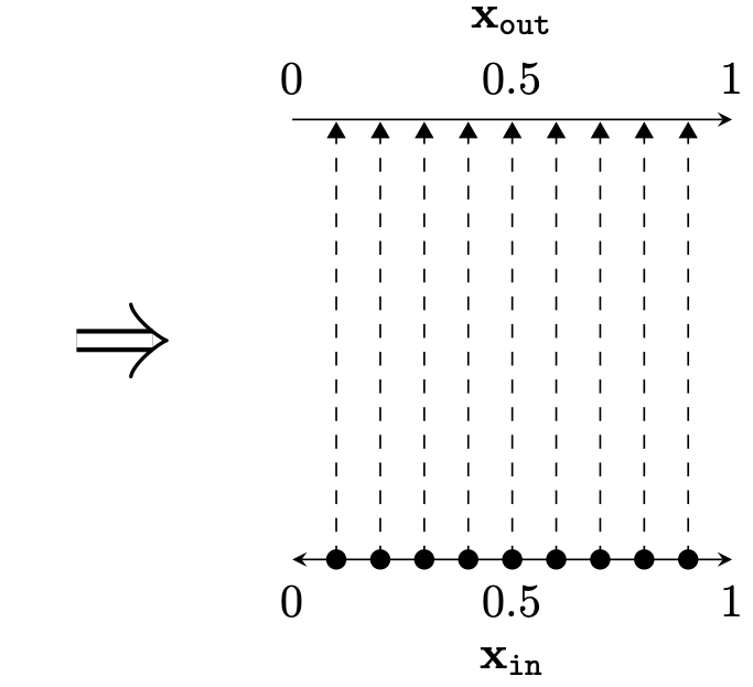
Two different ways to visualize a function

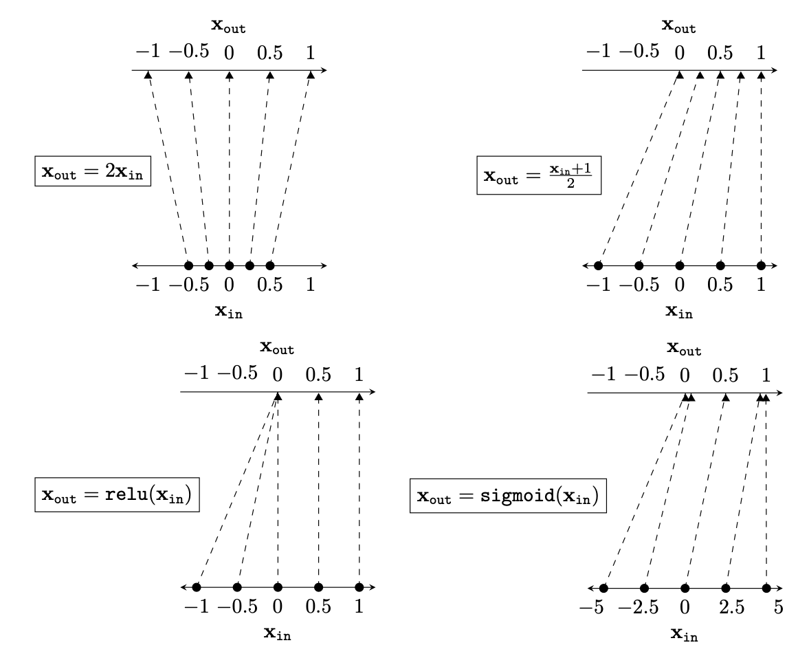
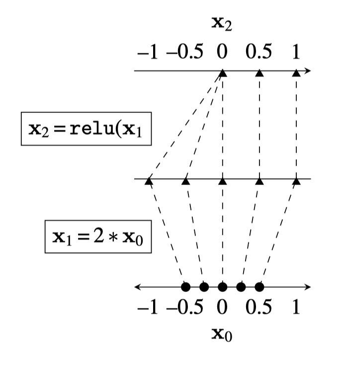
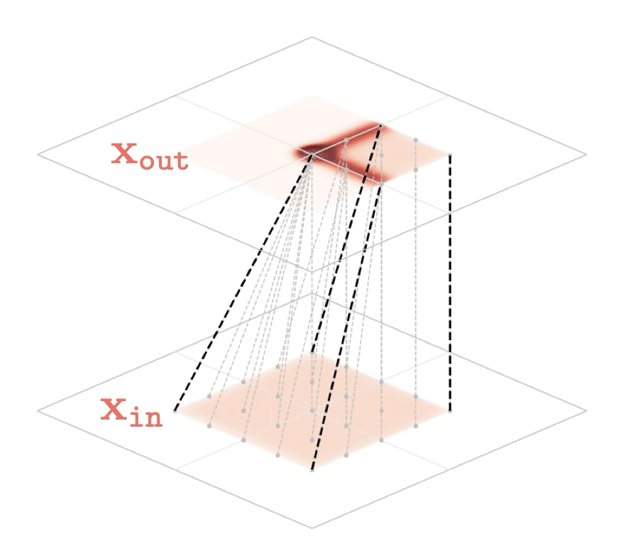
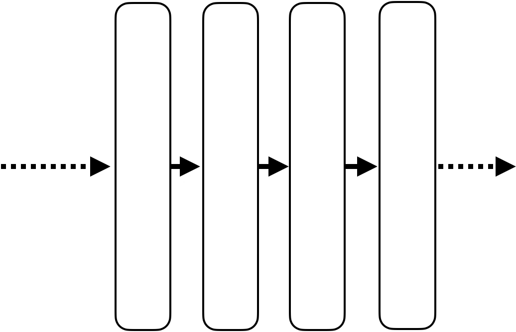
Representation transformations for a variety of neural net operations

and stack of neural net operations

)

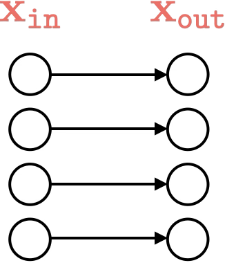
wiring graph

equation

mapping 1D

mapping 2D

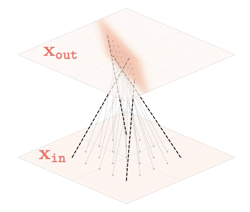
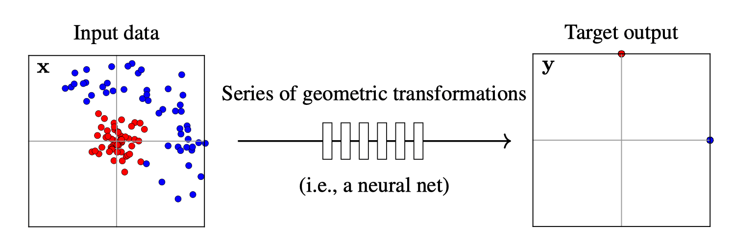
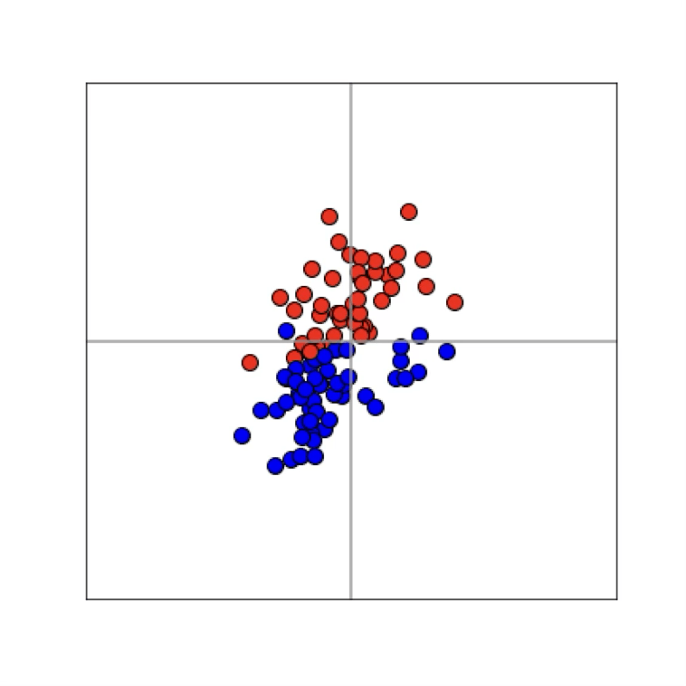
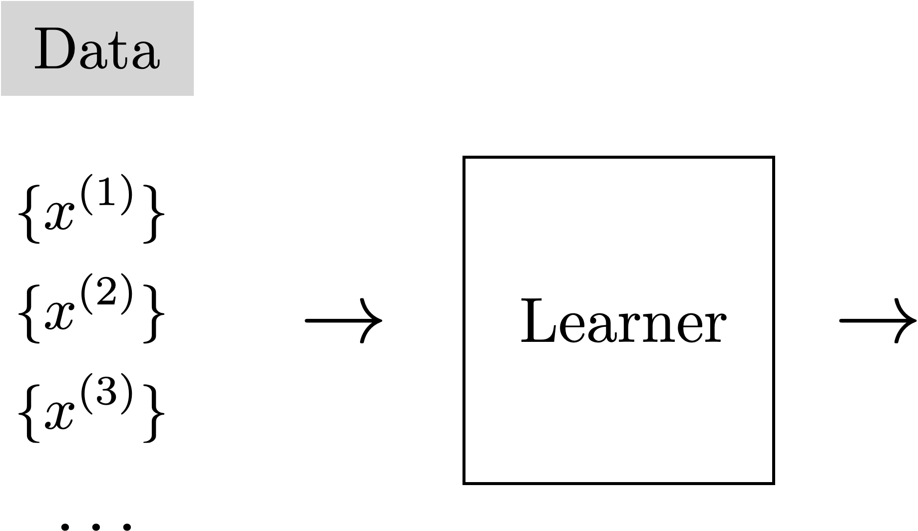
Training data

x

z_1

a_1

z_2

g

{z}_1=\text { linear }(x)

{a}_1=\text { ReLU}(z_1)

g=\text {softmax}(z_2)

{z}_2=\text { linear }(a_1)

x\in \mathbb{R^2}

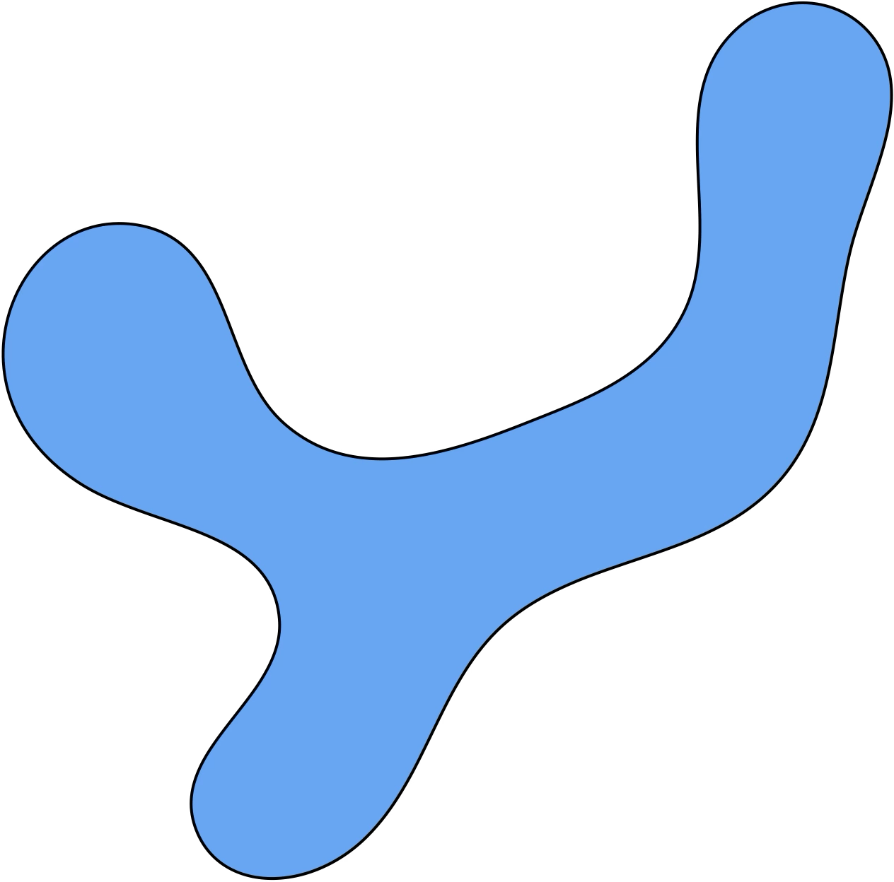
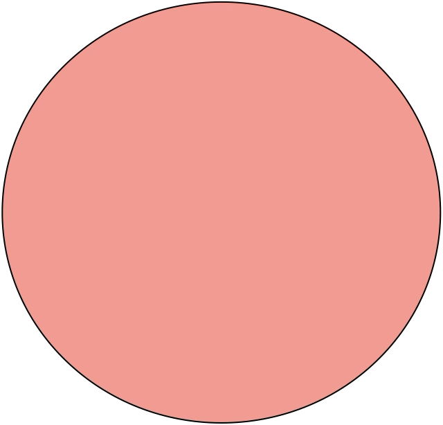
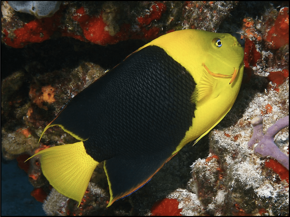
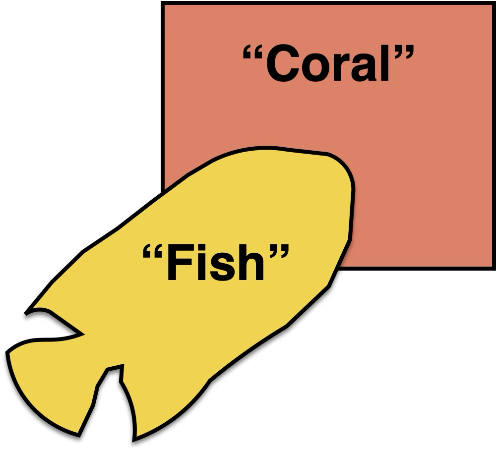
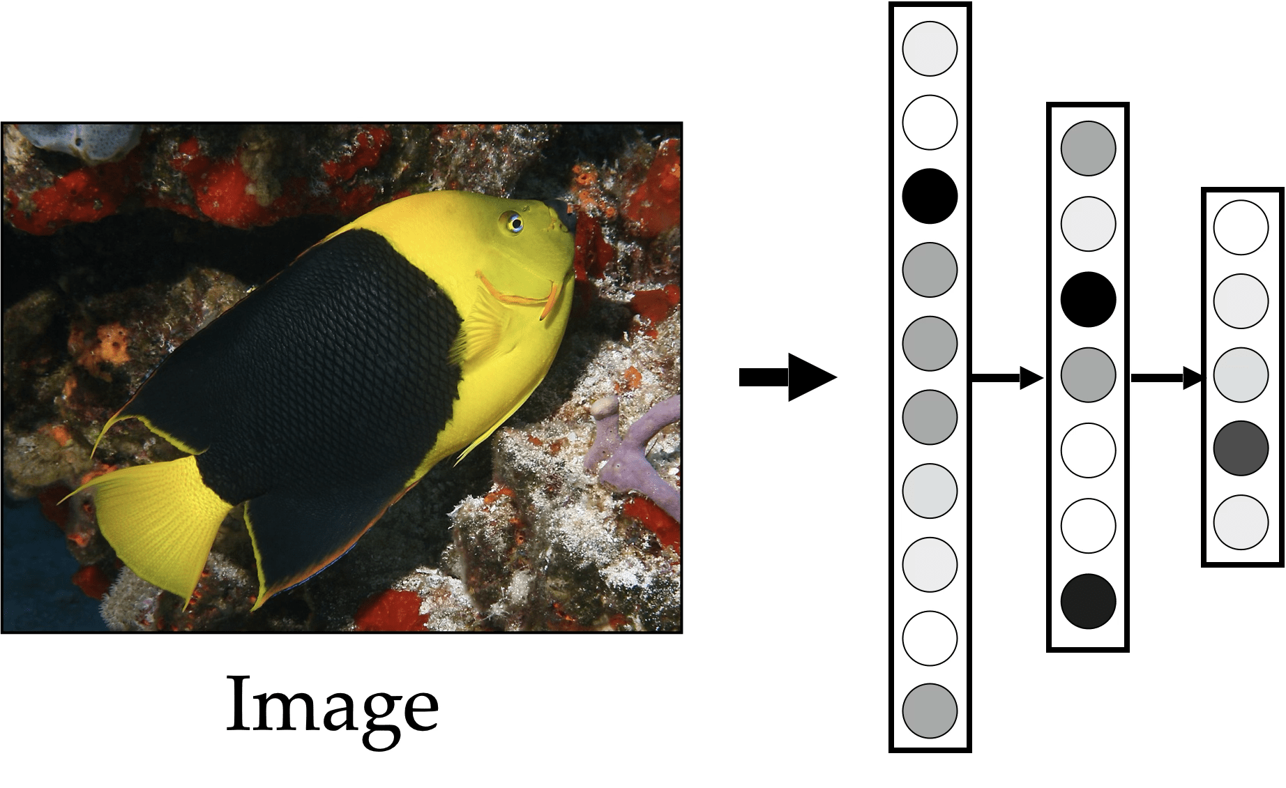
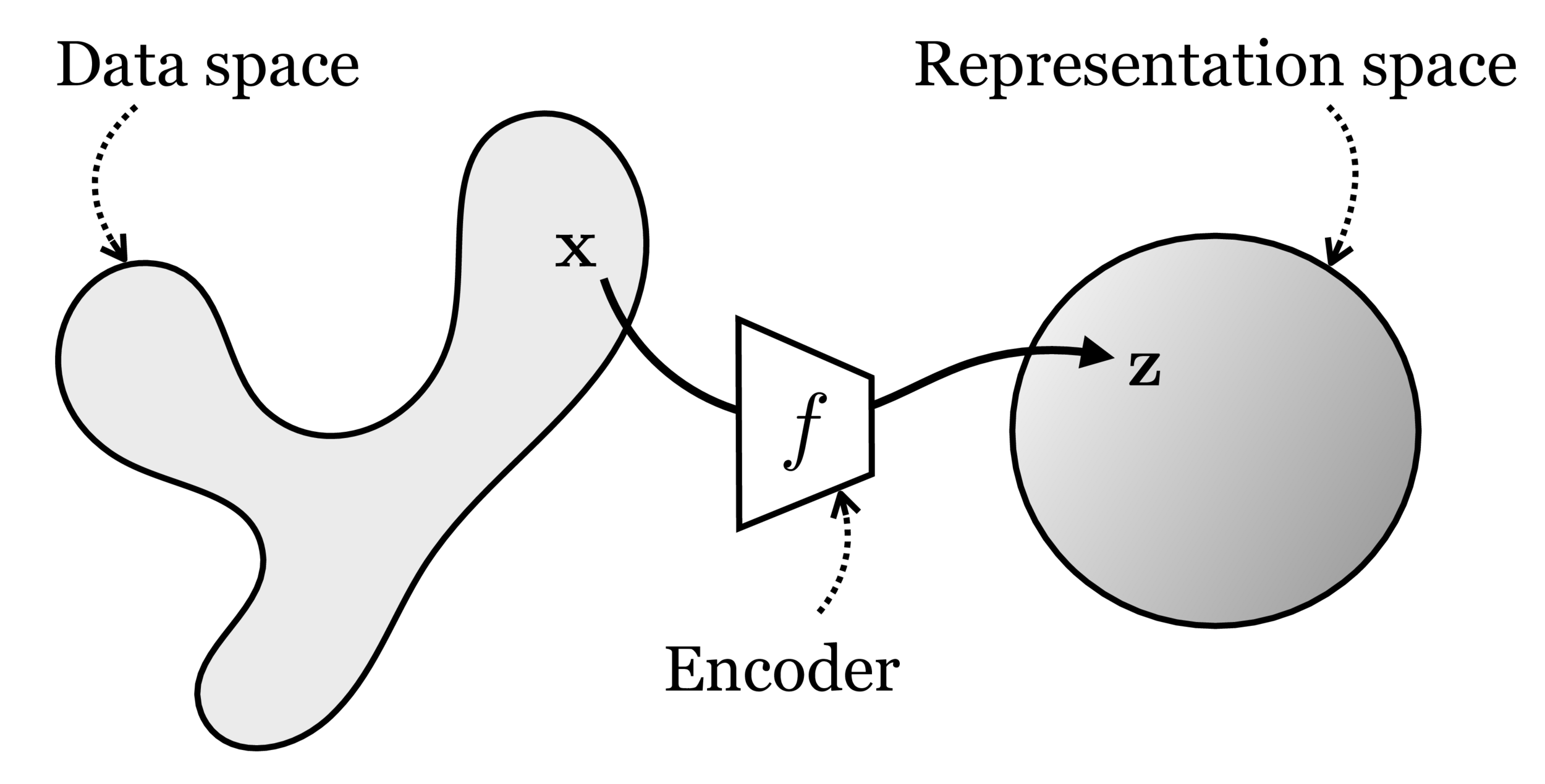
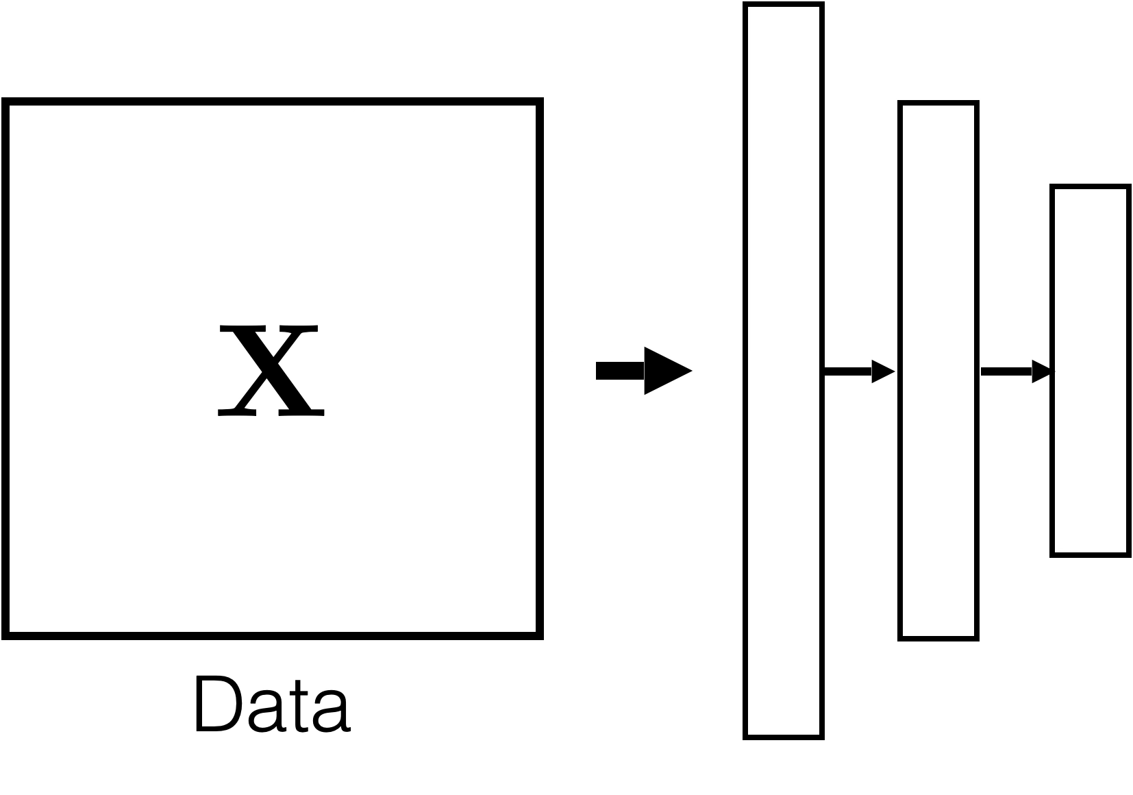
maps from complex data space to simple embedding space

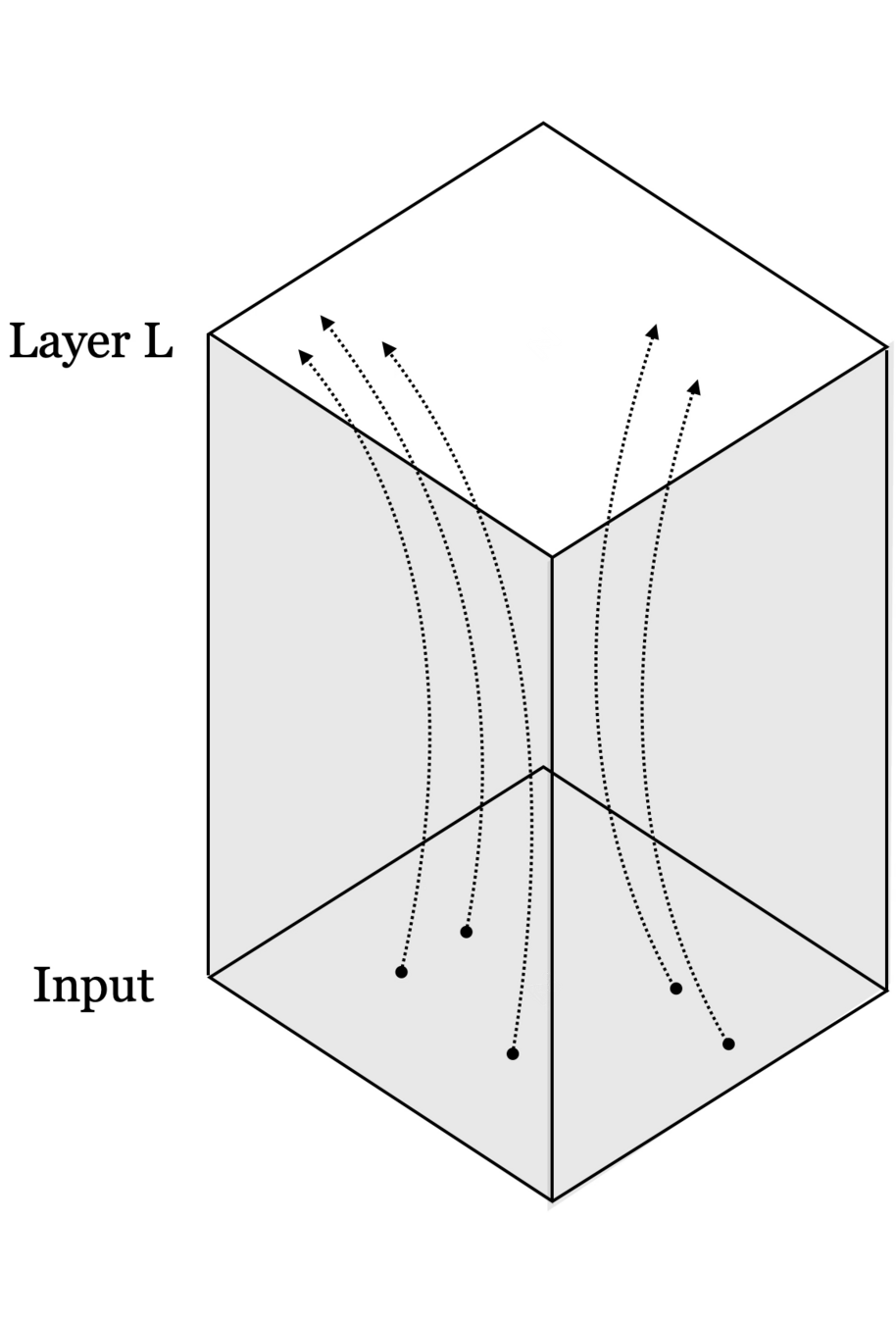
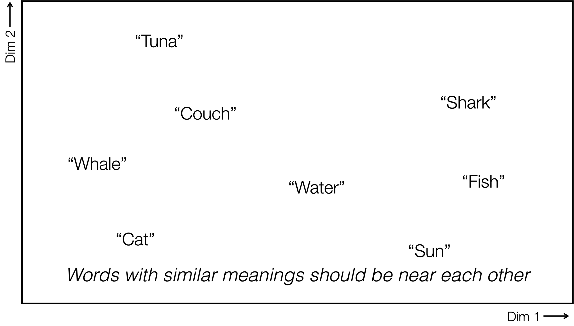
Neural networks are representation learners

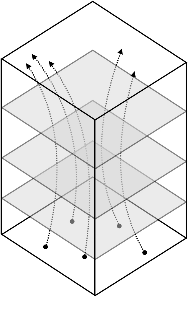
Deep nets transform datapoints, layer by layer
Each layer gives a different representation (aka embedding) of the data

🧠

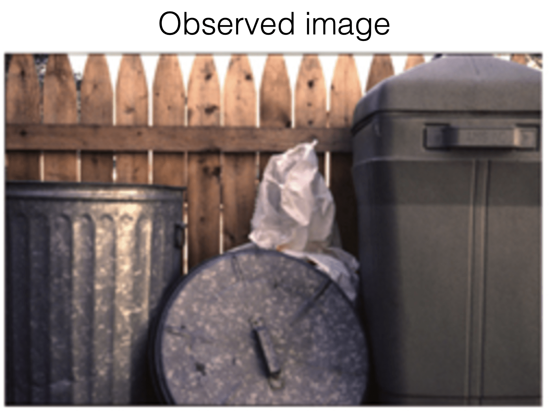
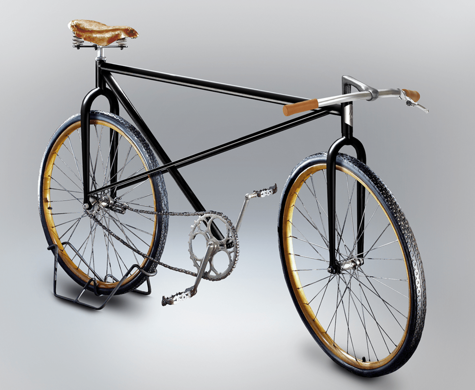
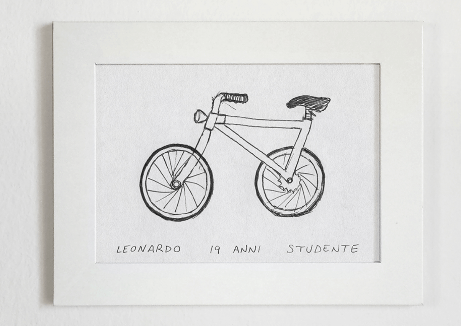
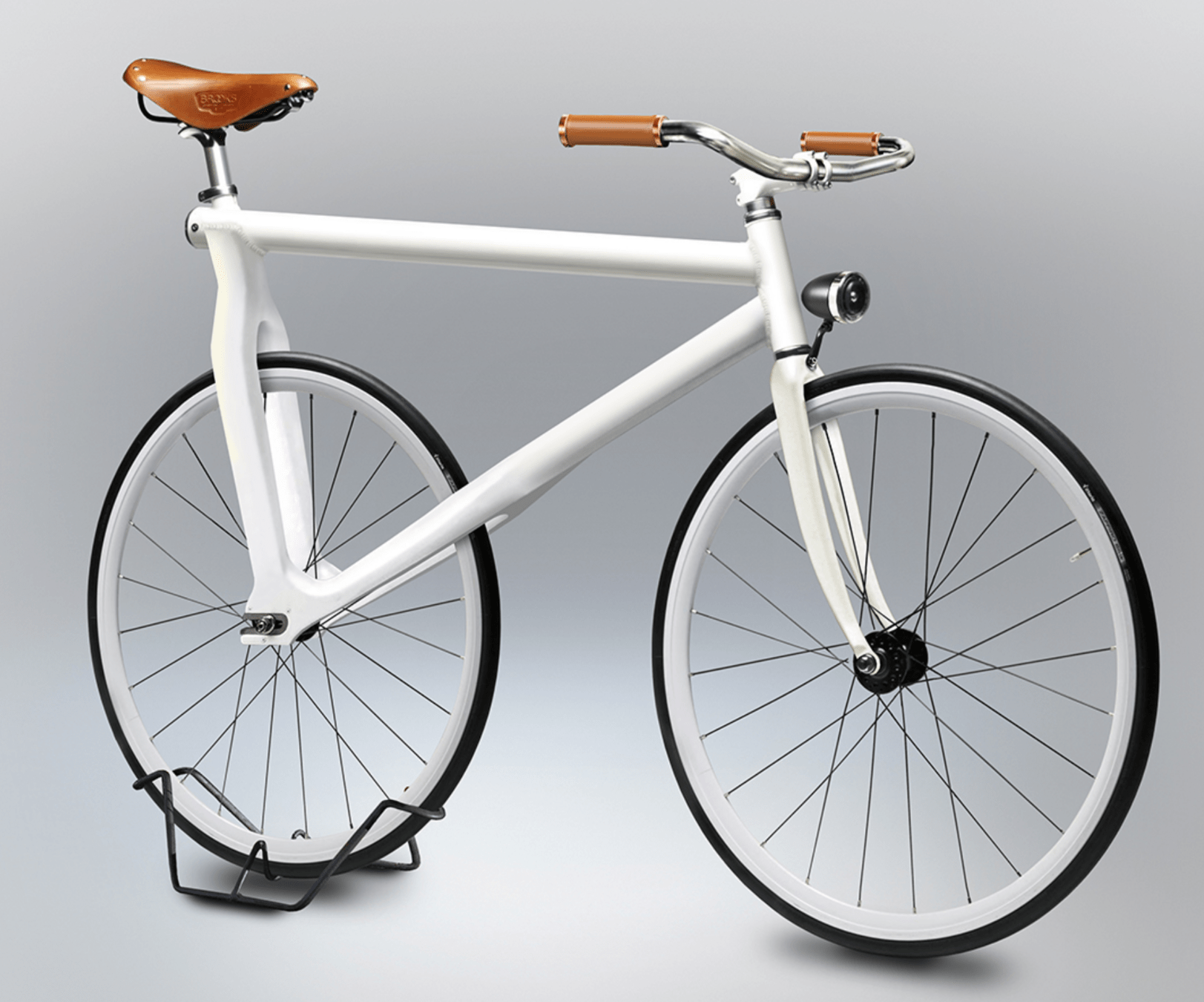
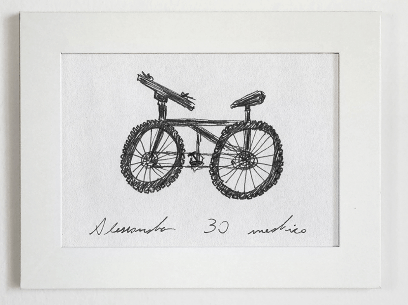
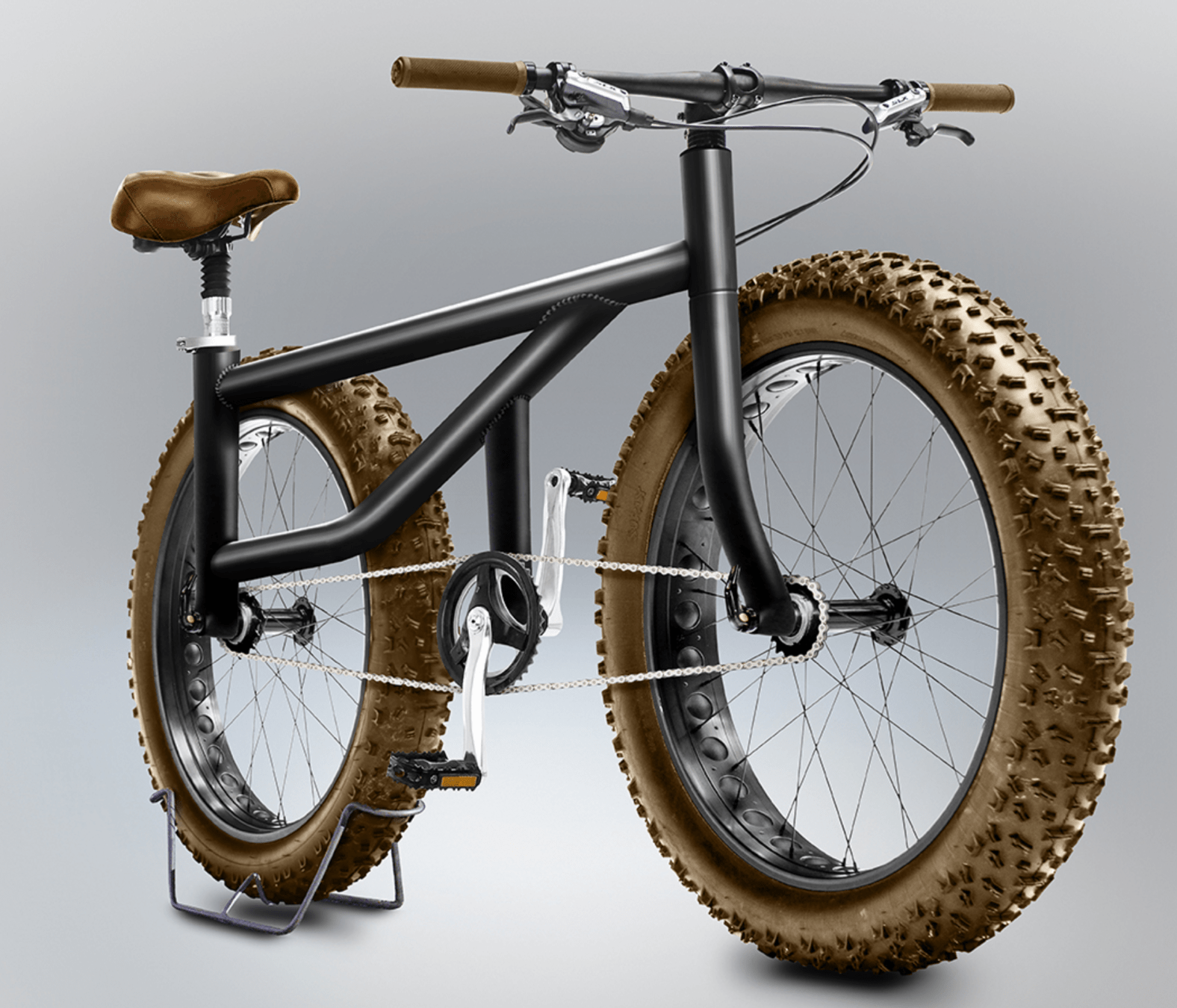
humans also learn representations

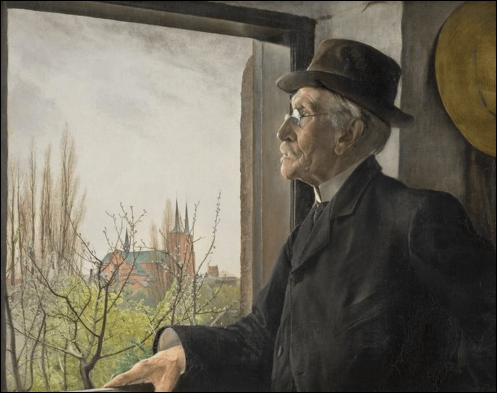
"I stand at the window and see a house, trees, sky. Theoretically I might say there were 327 brightnesses and nuances of colour. Do I have "327"? No. I have sky, house, and trees.”

— Max Wertheimer, 1923

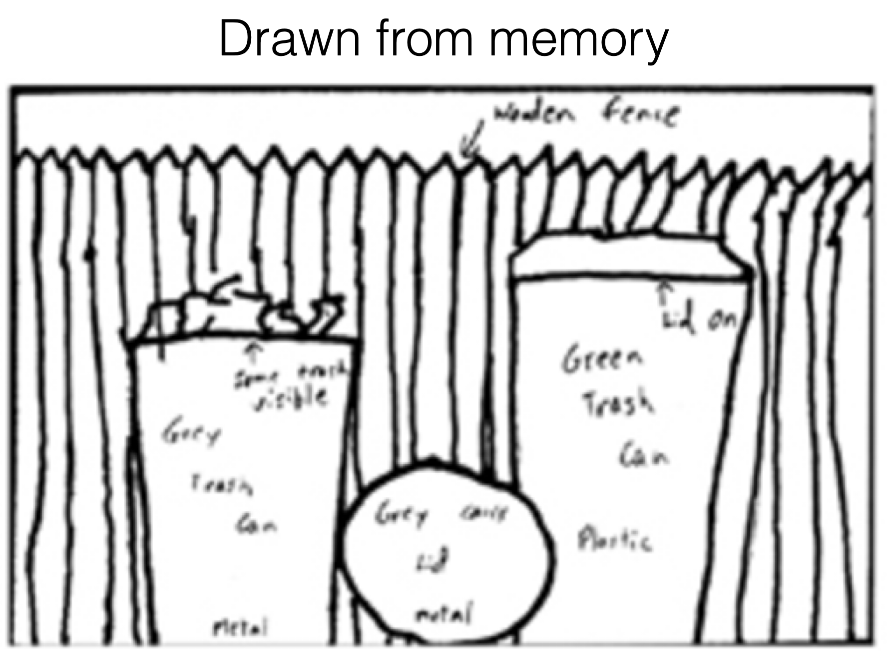
Good representations are:

Compact (minimal)
Explanatory (roughly sufficient)

[See “Representation Learning”, Bengio 2013, for more commentary]

[Bartlett, 1932]
[Intraub & Richardson, 1989]

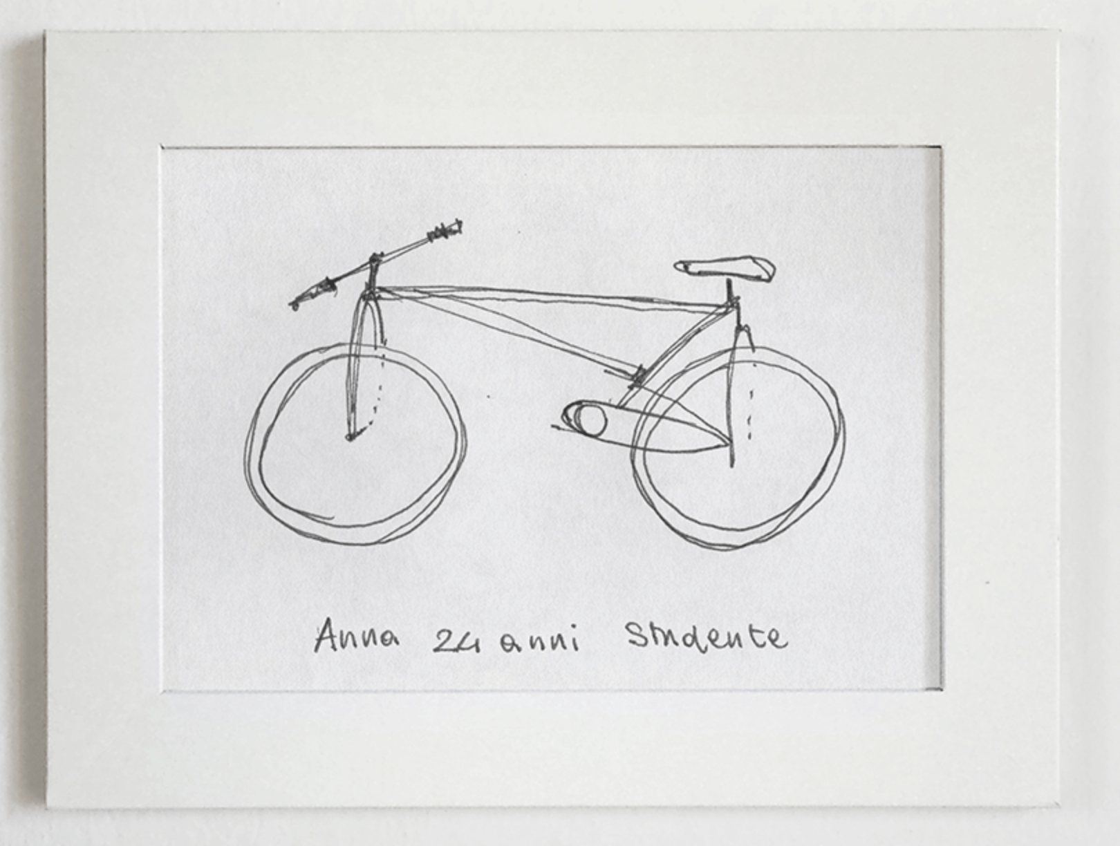
[https://www.behance.net/gallery/35437979/Velocipedia]

Outline

Recap, neural networks mechanism
Neural networks are representation learners
Auto-encoder:
- Bottleneck
- Reconstruction
Unsupervised learning
(Some recent representation learning ideas)

Compact (minimal)
Explanatory (roughly sufficient)
Disentangled (independent factors)
Interpretable
Make subsequent problem solving easy

[See “Representation Learning”, Bengio 2013, for more commentary]

Auto-encoders try to achieve these

\left\{ \begin{array}{l} \\ \\ \end{array} \right.

\left\{ \begin{array}{l} \\ \\ \\ \end{array} \right.

these may just emerge as well

Good representations are:

compact representation/embedding

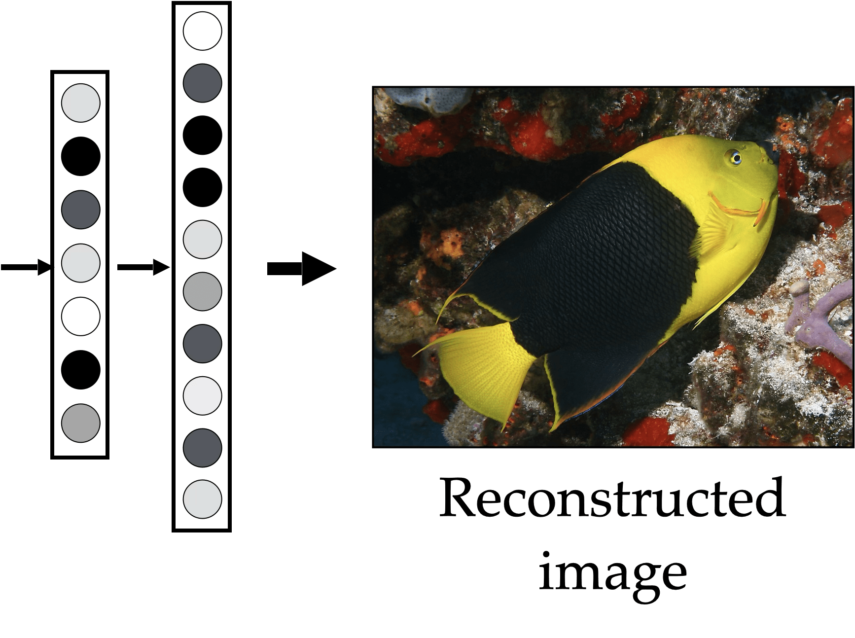
Auto-encoder

"What I cannot create, I do not understand." Feynman

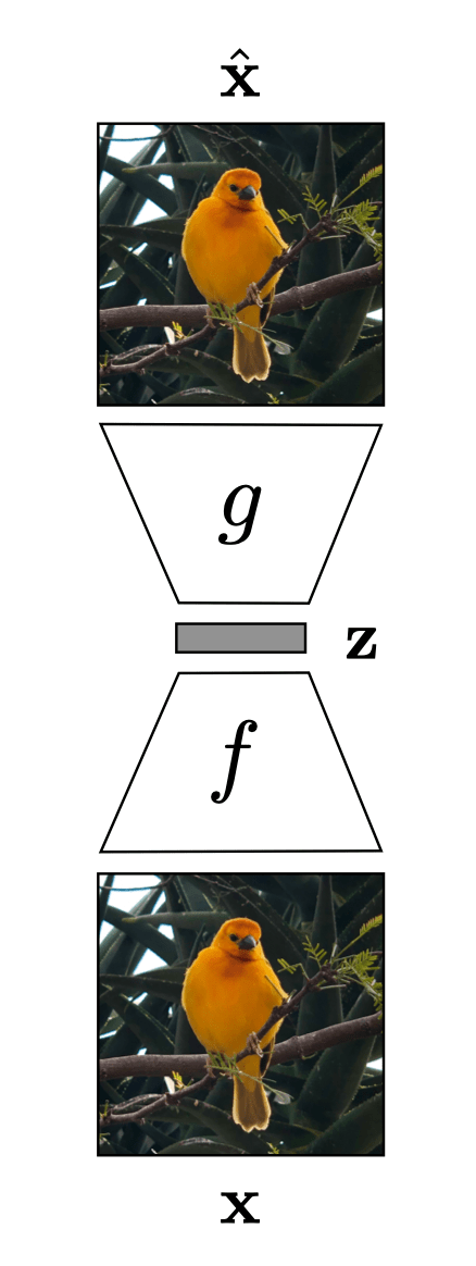
Auto-encoder

\underbrace{\hspace{1cm}}

encoder

decoder

bottleneck

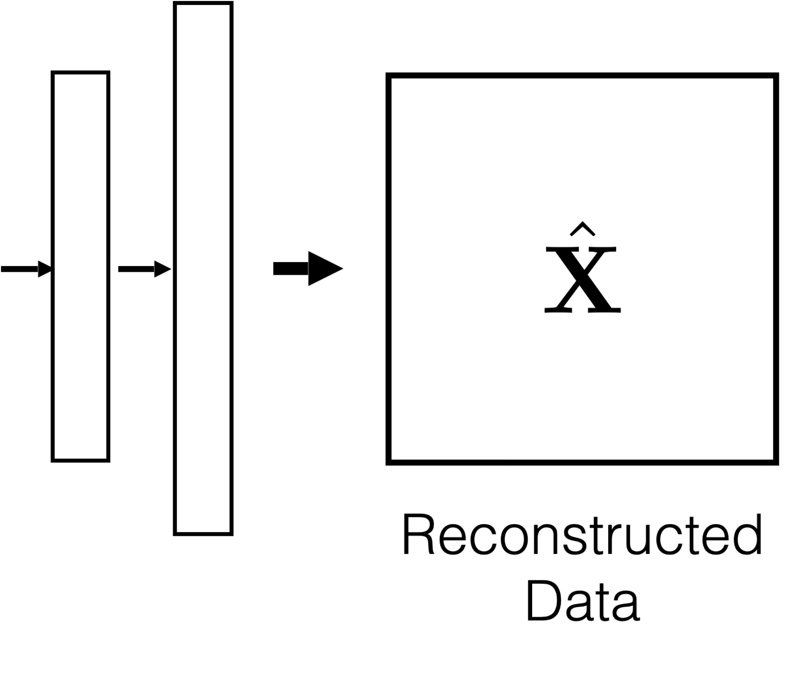
Auto-encoder

x

\tilde{x}=\text{NN}(x;W)

\min_{W} ||x - \tilde{x}||^2

input \(x \in \mathbb{R^d}\)

output \(\tilde{x} \in \mathbb{R^d}\)

\dots

bottleneck

typically, has lower dimension than \(d\)

Auto-encoder

Training Data

\left\{{x}^{(i)}\right\}_{i=1}^n

loss/objective

\mathcal{L}(F(\mathbf{x}), \mathbf{x})=\|F(\mathbf{x})-\mathbf{x}\|^2

hypothesis class

A model

\(f\)

F=g \circ h: \mathbb{R}^d \rightarrow \mathbb{R}^m \rightarrow \mathbb{R}^d

h

g

\(m<d\)

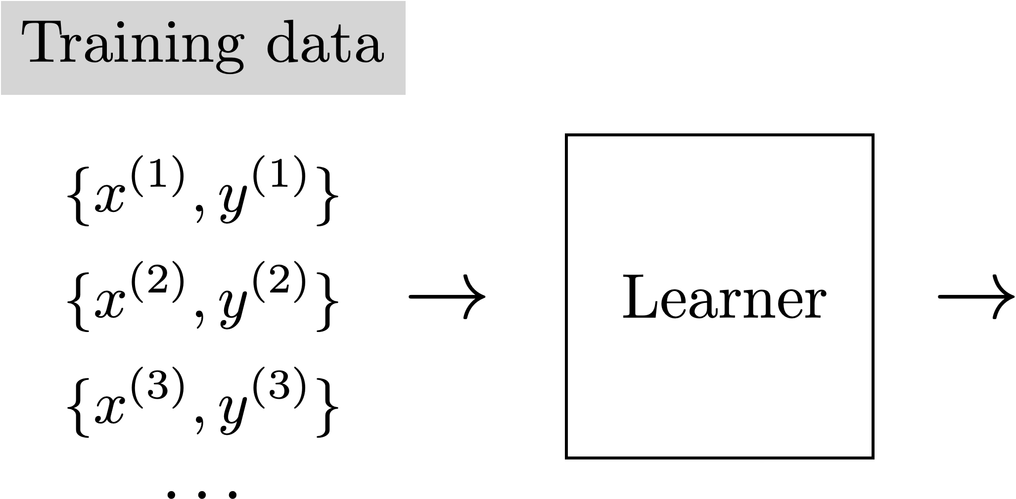
\(f: X \rightarrow Y\)

Supervised Learning

"Good"

Representation

Unsupervised Learning

Training Data

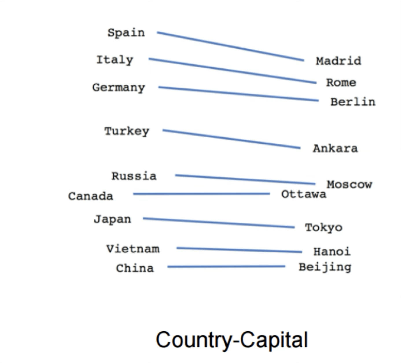
Word2Vec

https://www.tensorflow.org/text/tutorials/word2vec

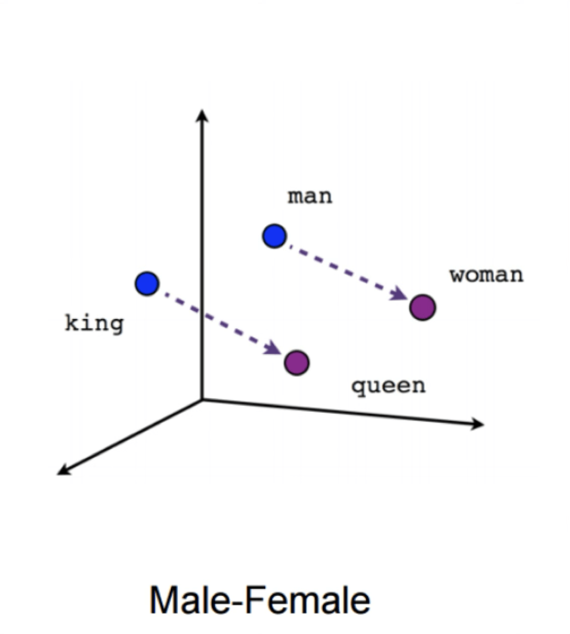
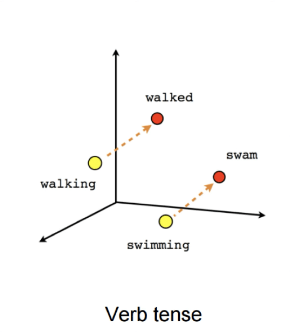
Word2Vec

verb tense

gender

X = Vector(“Paris”) – vector(“France”) + vector(“Italy”) \(\approx\) vector("Rome")

“Meaning is use” — Wittgenstein

Can help downstream tasks:

sentiment analysis
machine translation
info retrieval

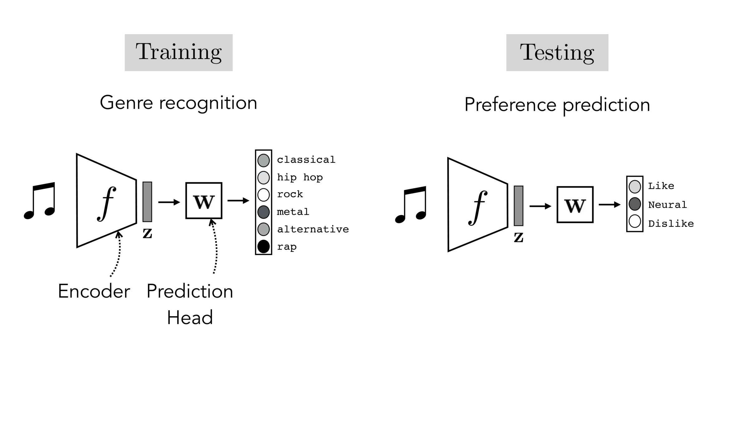
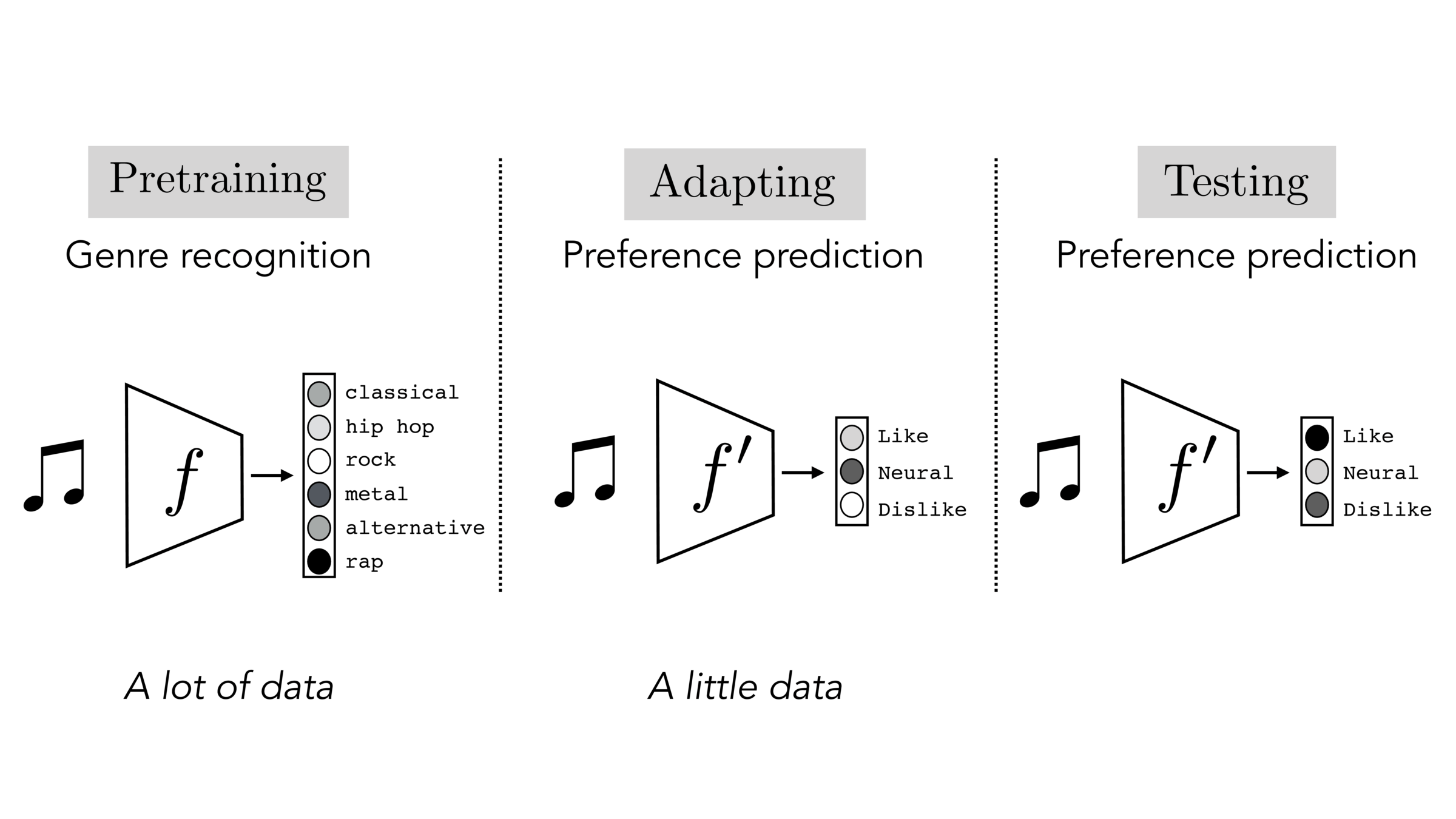
Often, what we will be “tested” on is not what we were trained on.

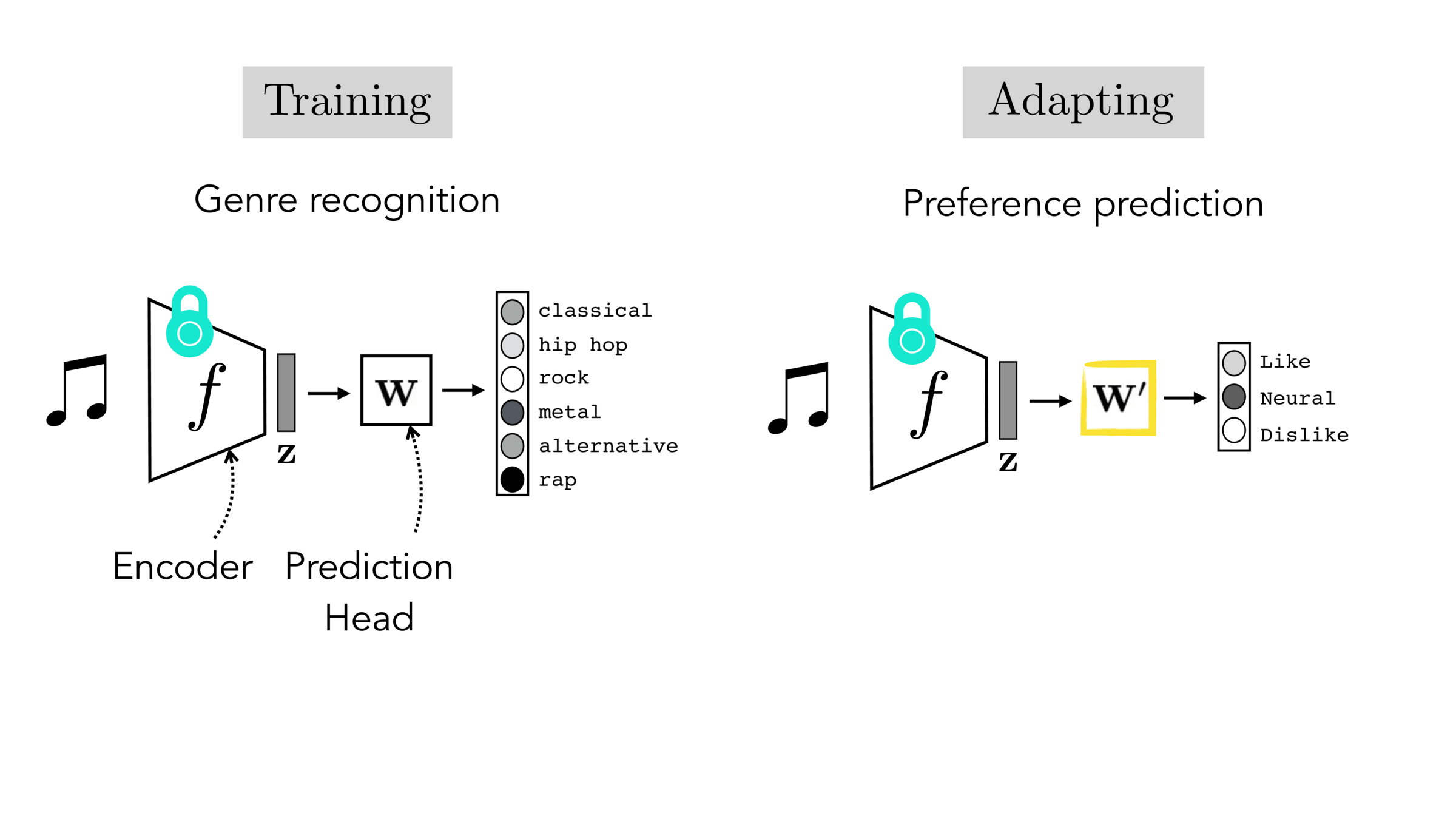
Final-layer adaptation: freeze \(f\), train a new final layer to new target data

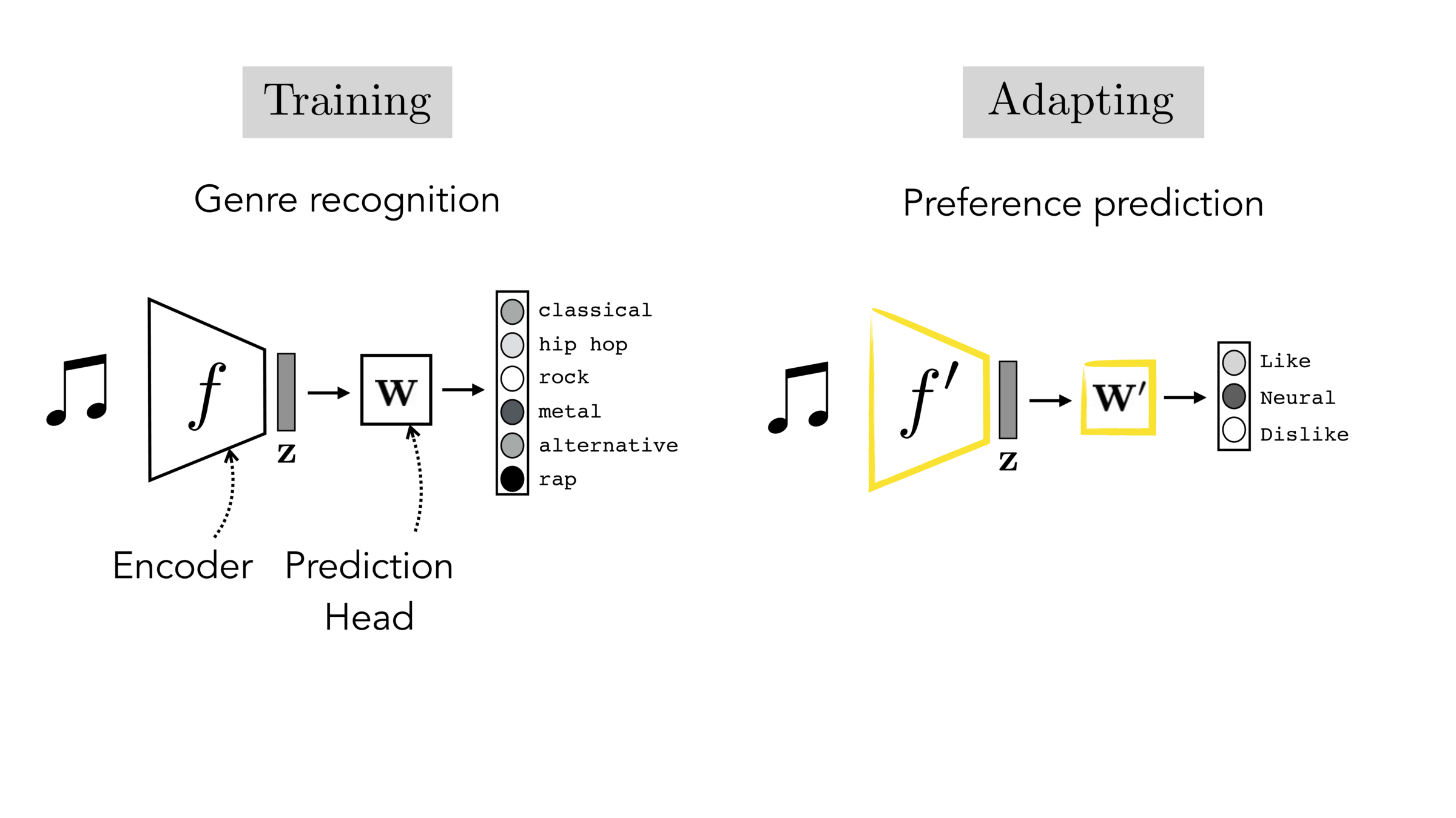
Finetuning: initialize \(f’\) as \(f\), then continue training for \(f'\) as well, on new target data

Outline

Recap, neural networks mechanism
Neural networks are representation learners
Auto-encoder:
- Bottleneck
- Reconstruction
Unsupervised learning
(Some recent representation learning ideas)

\left( \begin{array}{l} \\ \\ \\ \\ \\ \\ \end{array} \right.

Feature reconstruction (unsupervised learning)

Features

Reconstructed Features

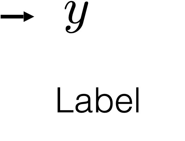
Label prediction (supervised learning)

Features

Label

Partial

features

Other partial

features

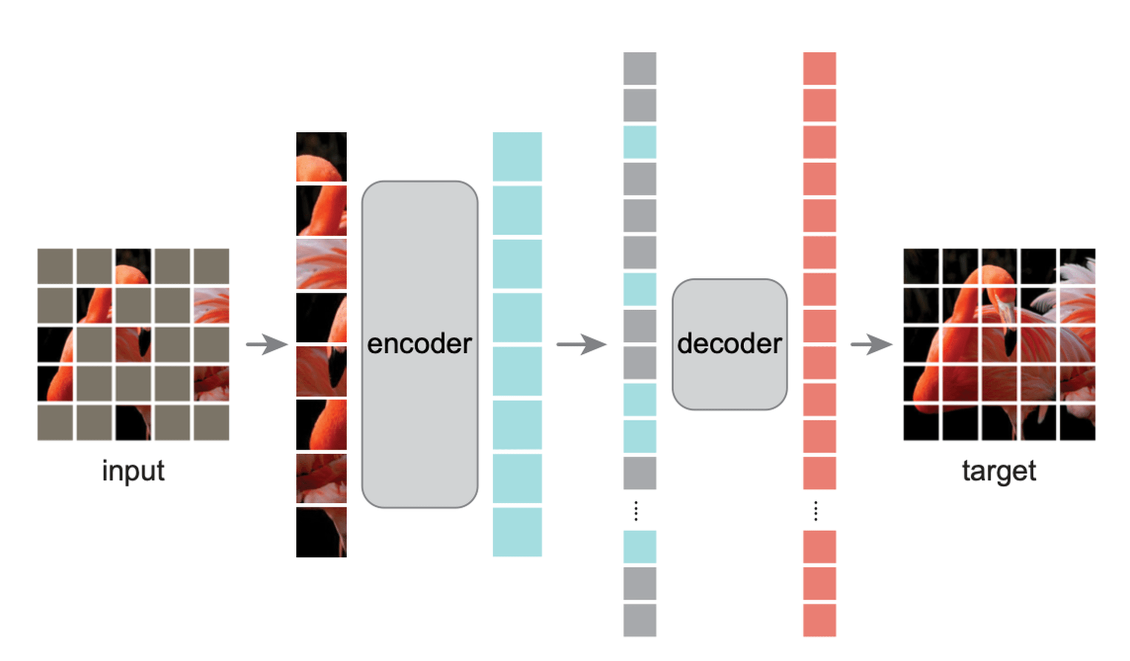
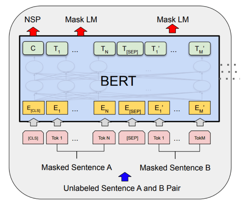
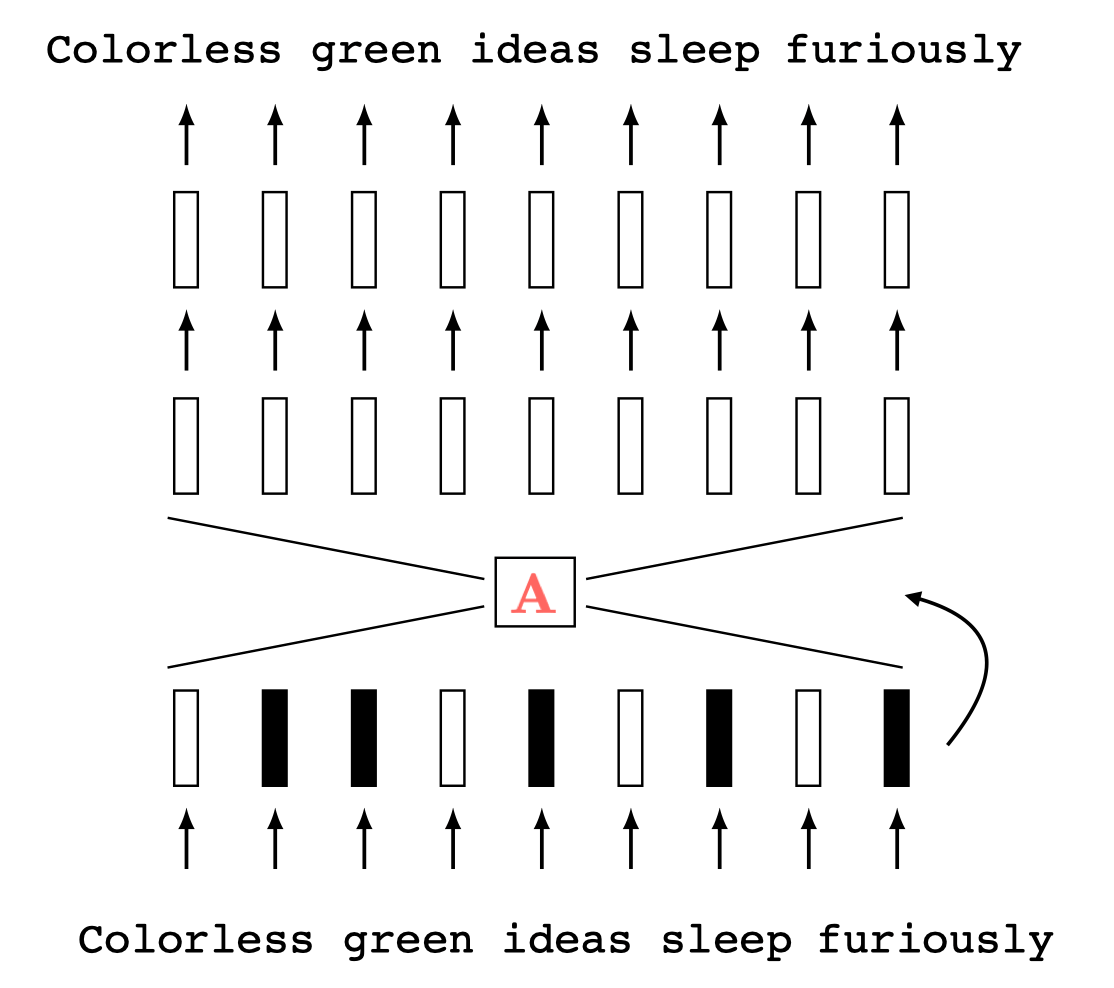
Masked Auto-encoder

[He, Chen, Xie, et al. 2021]

Masked Auto-encoder

[Devlin, Chang, Lee, et al. 2019]

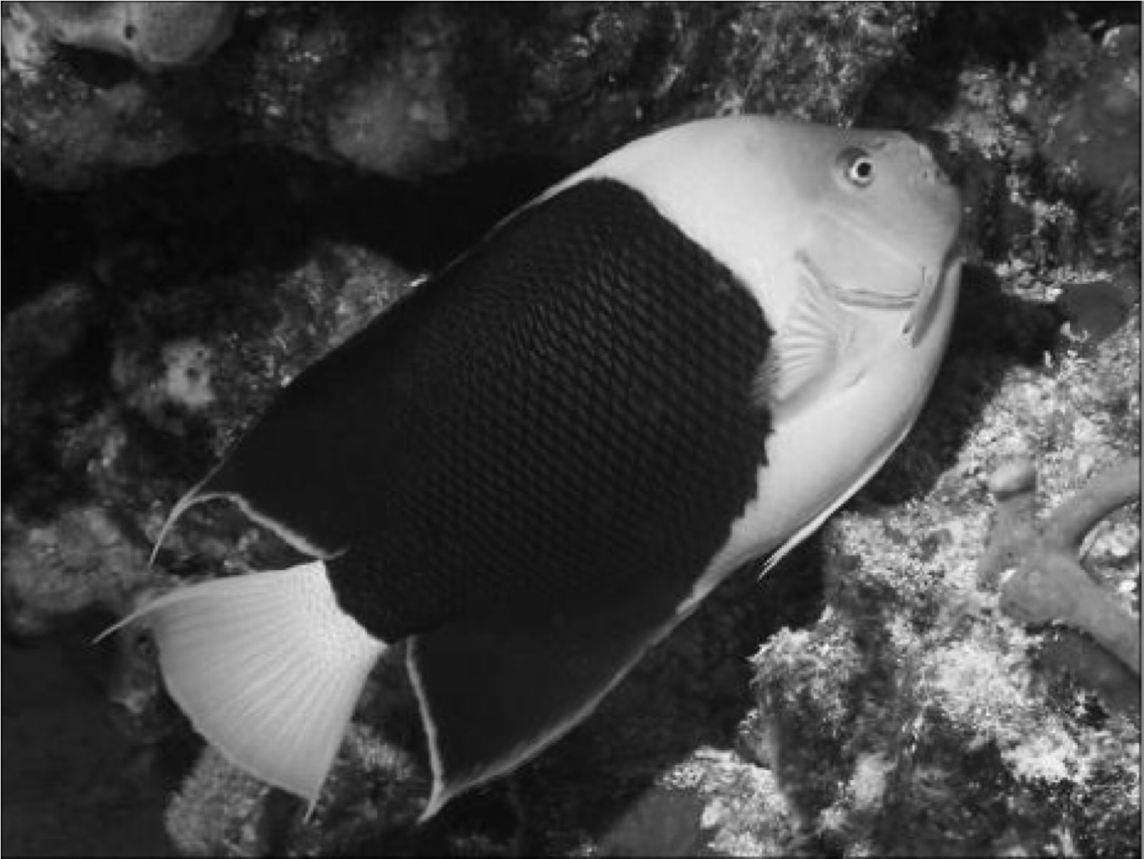
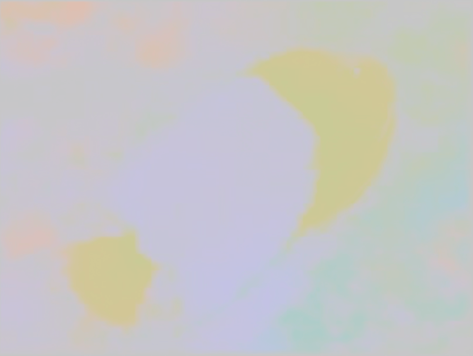
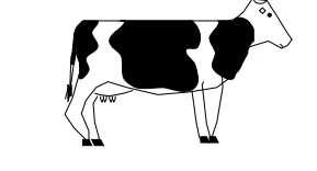
[Zhang, Isola, Efros, ECCV 2016]

predict color from gray-scale

[Zhang, Isola, Efros, ECCV 2016]

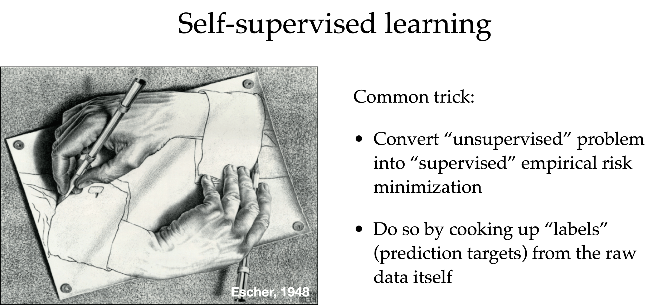
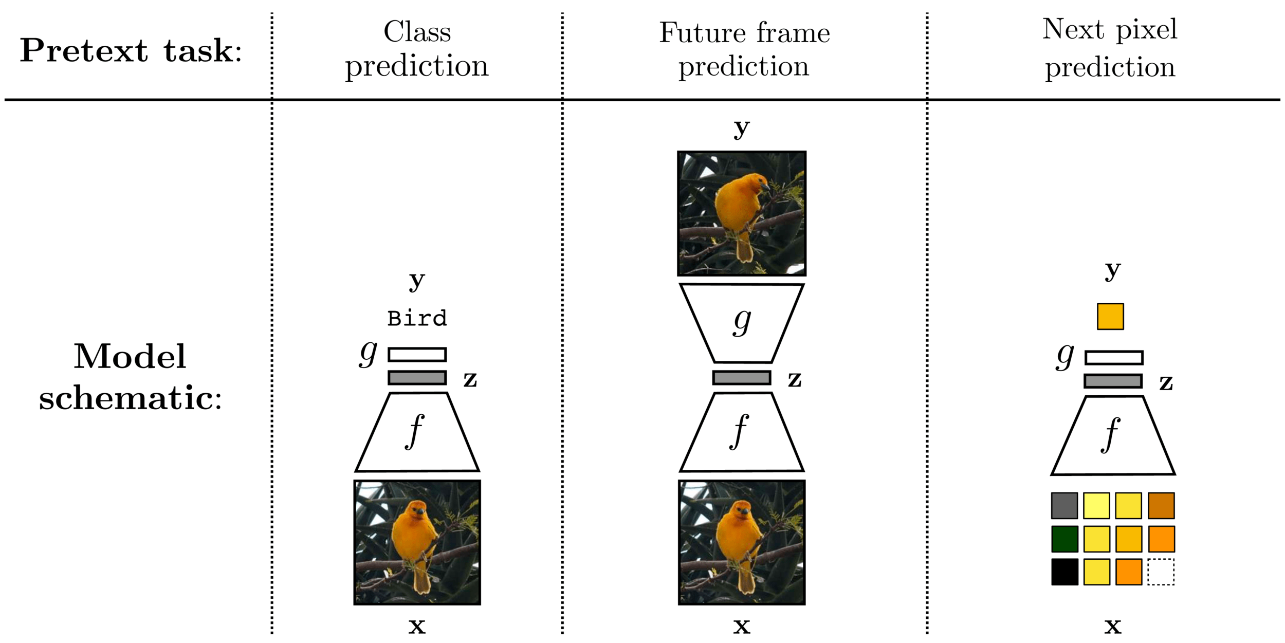
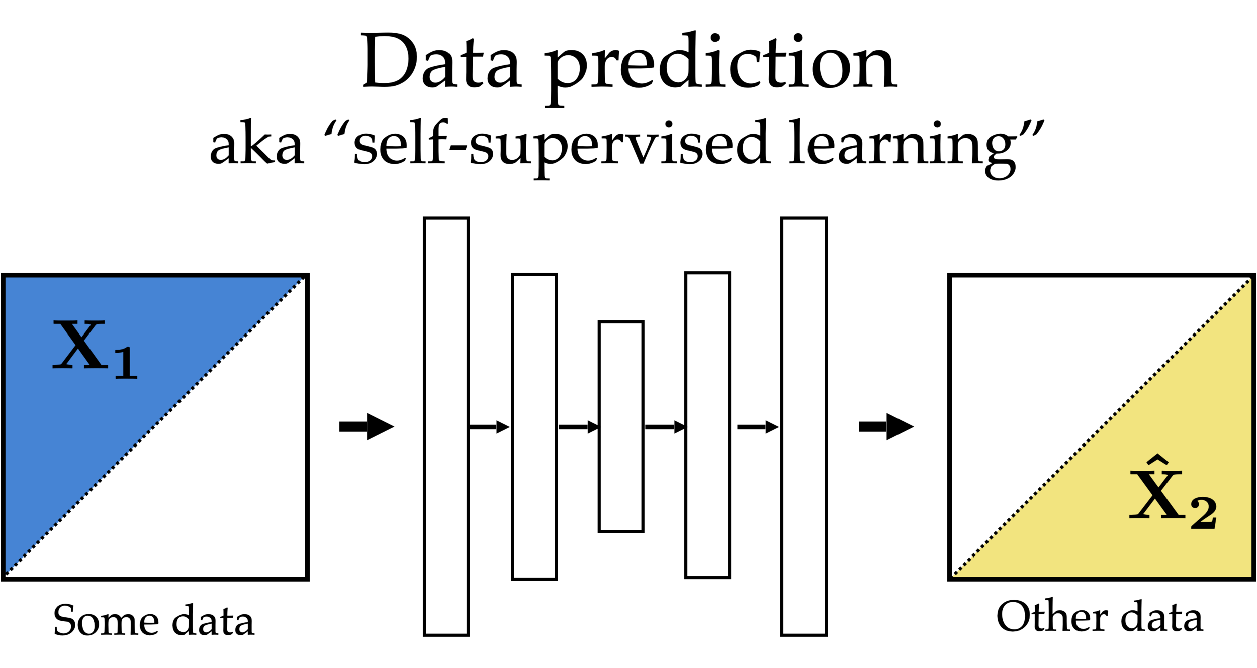
Self-supervised learning

Common trick:

Convert “unsupervised” problem into “supervised” setup
Do so by cooking up “labels” (prediction targets) from the raw data itself — called pretext task

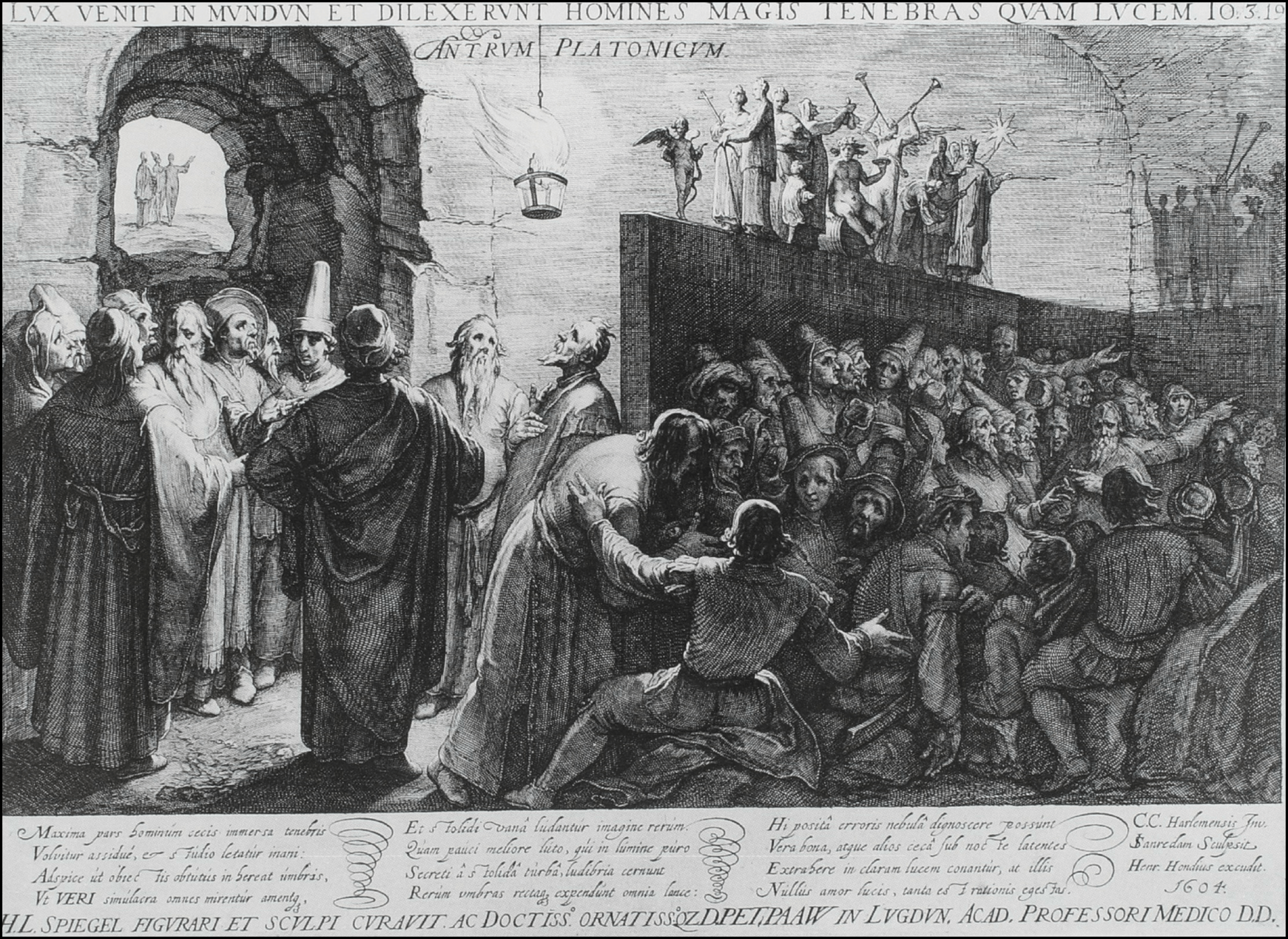
The allegory of the cave

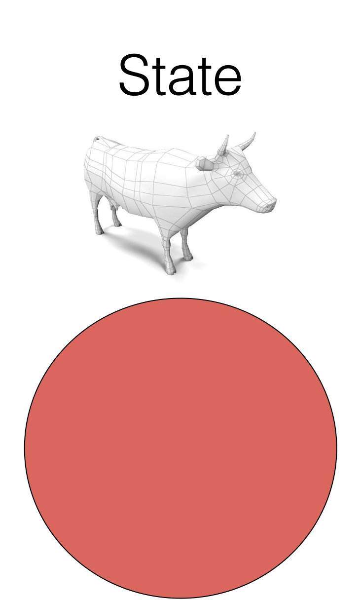
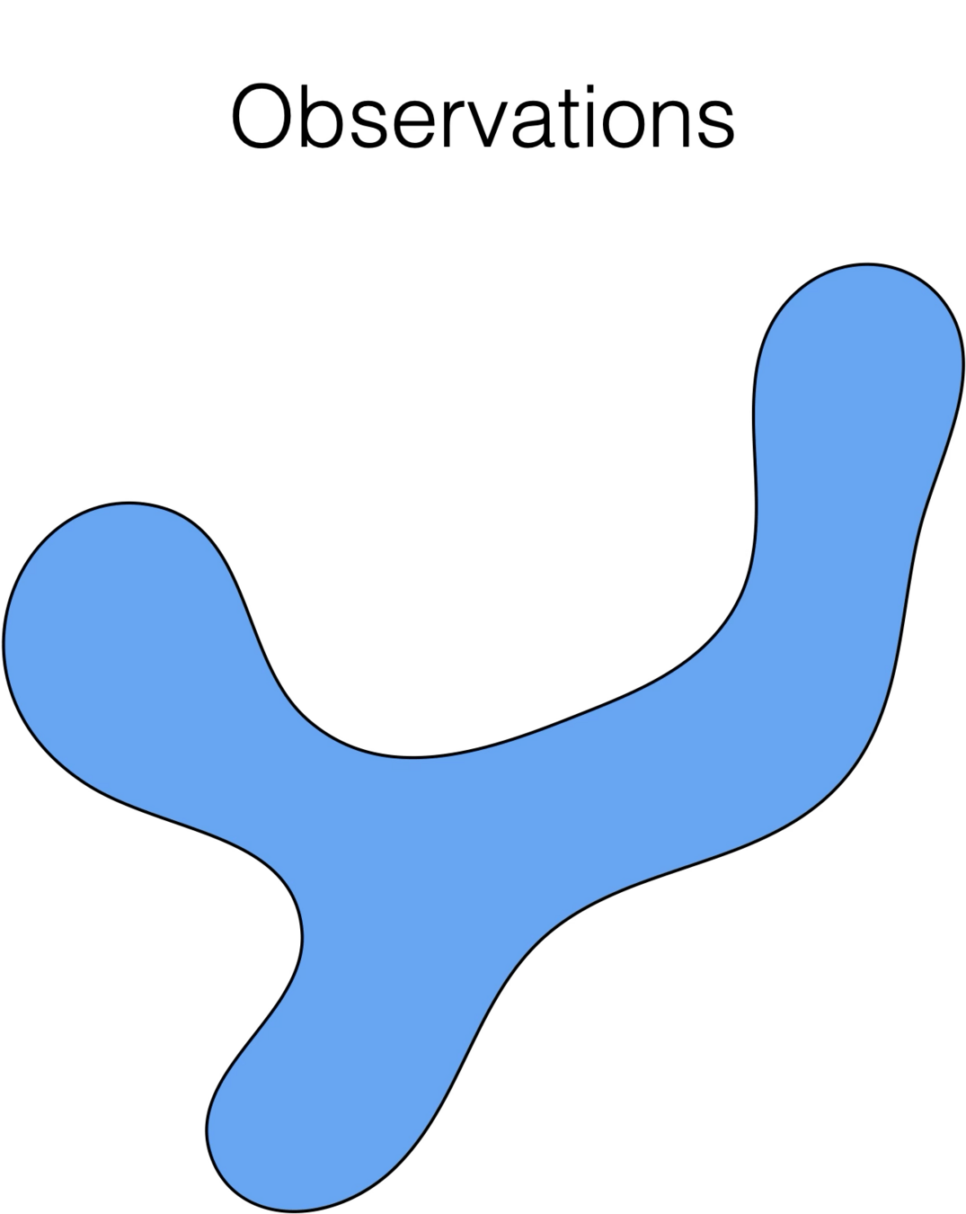
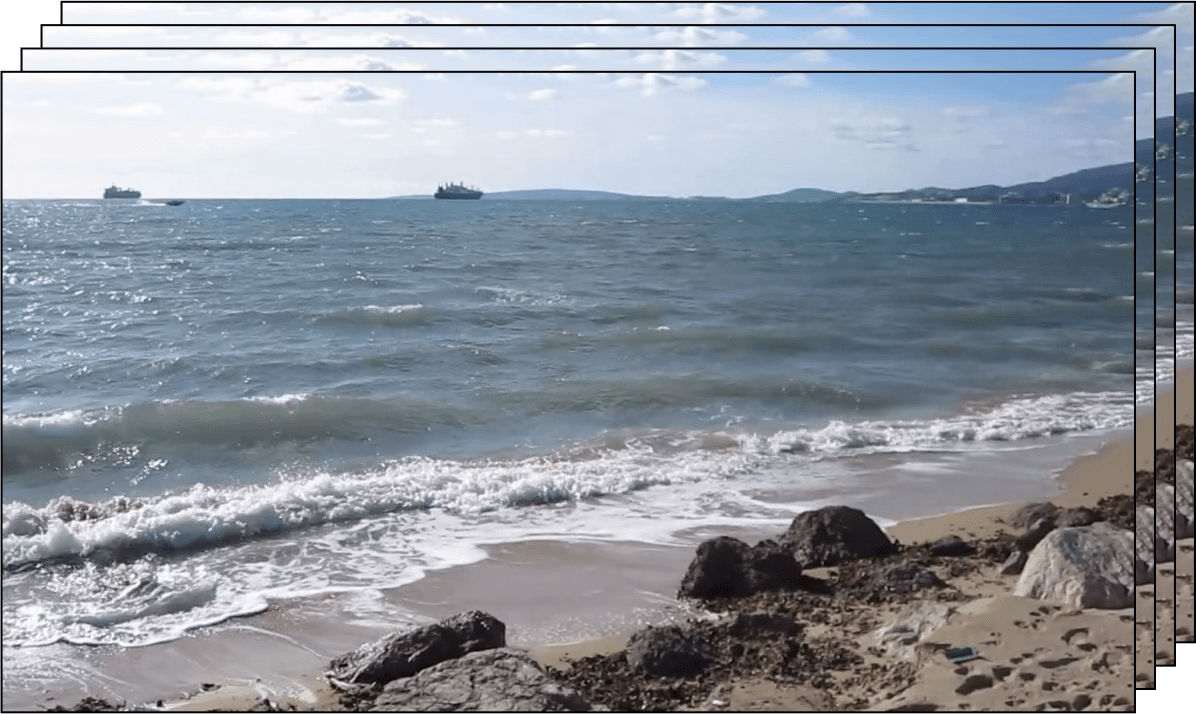
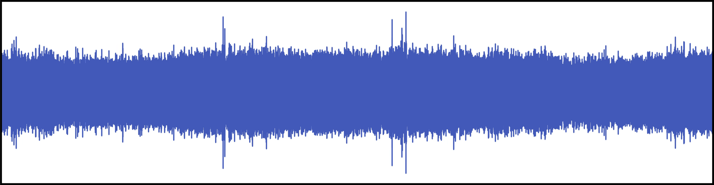
[Slide credit: Andrew Owens]

[Owens et al, Ambient Sound Provides Supervision for Visual Learning, ECCV 2016]

[Slide credit: Andrew Owens]

[Owens et al, Ambient Sound Provides Supervision for Visual Learning, ECCV 2016]

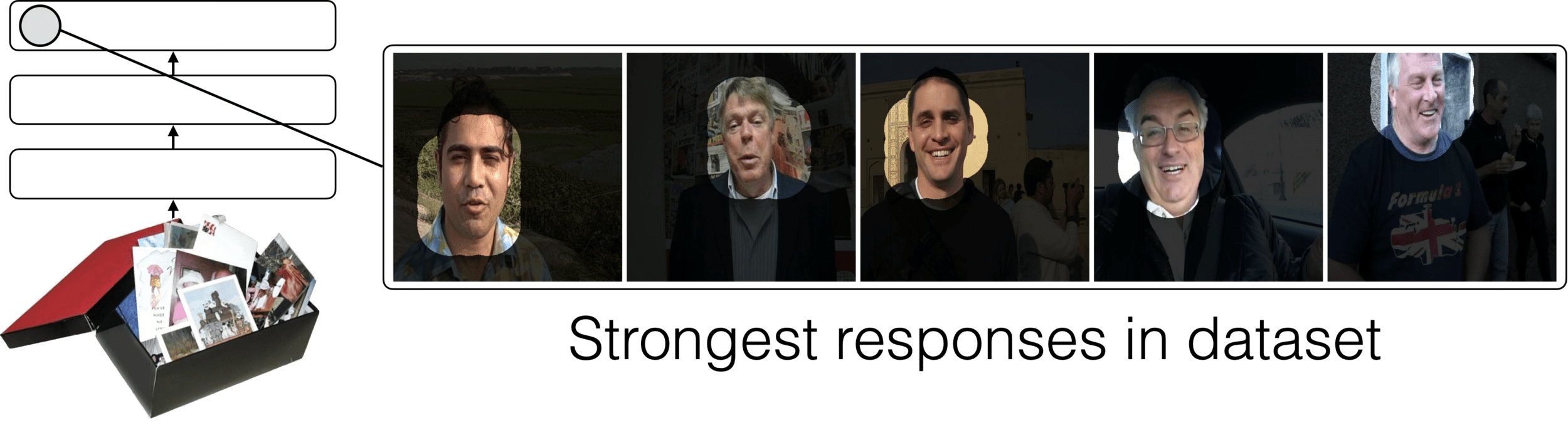
What did the model learn?

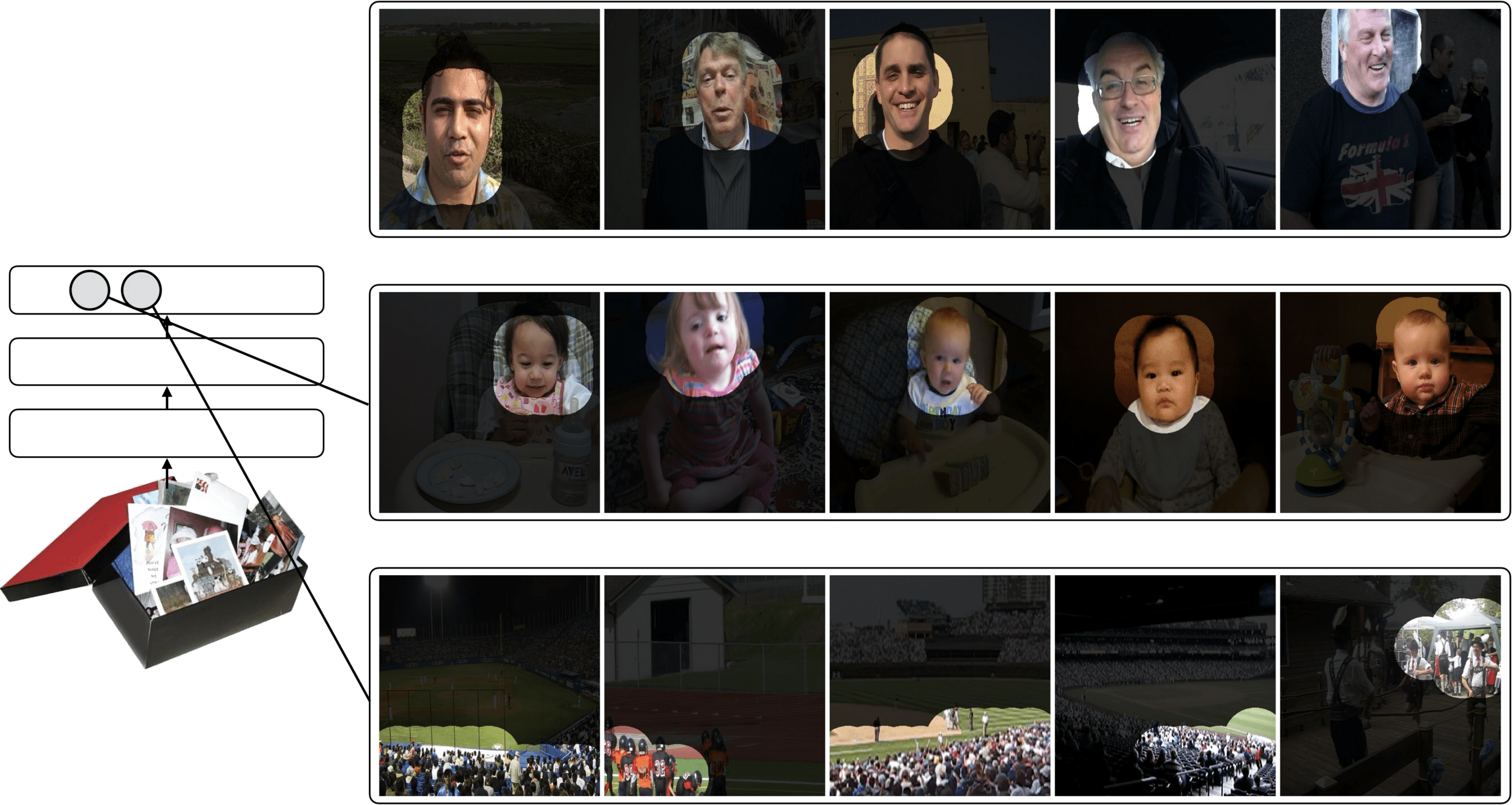
[Slide credit: Andrew Owens]

[Owens et al, Ambient Sound Provides Supervision for Visual Learning, ECCV 2016]

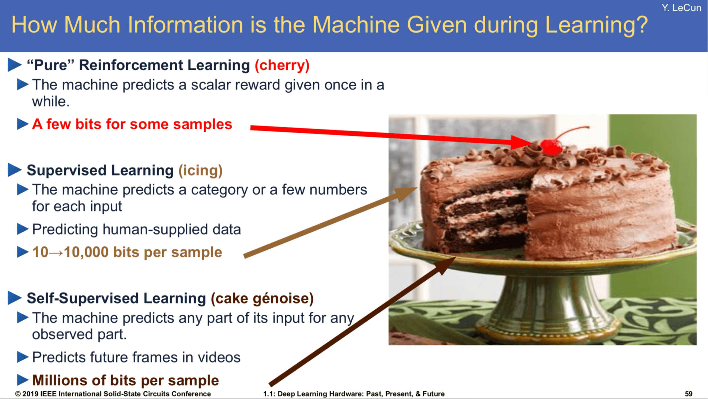
[Slide Credit: Yann LeCun]

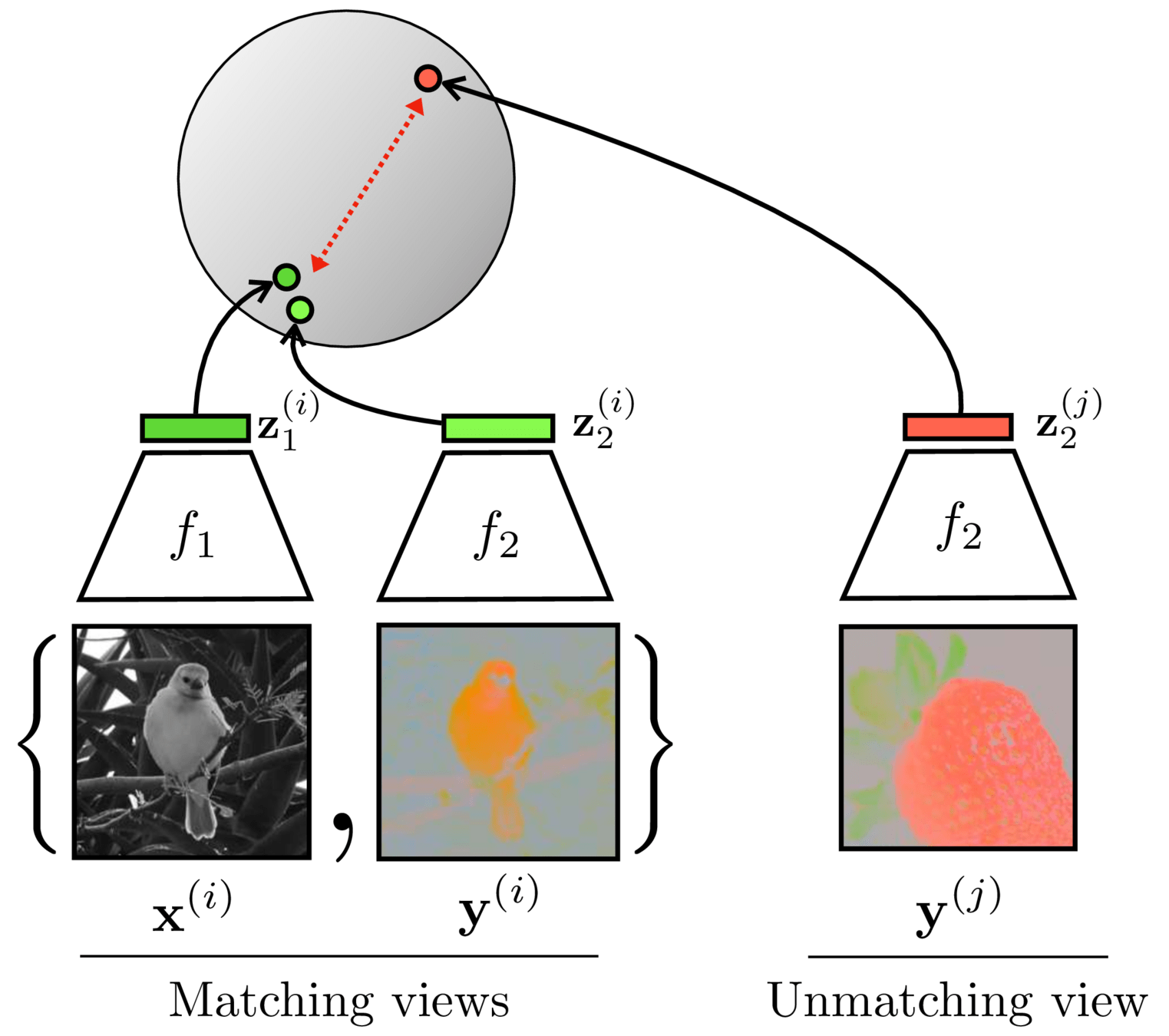
Contrastive learning

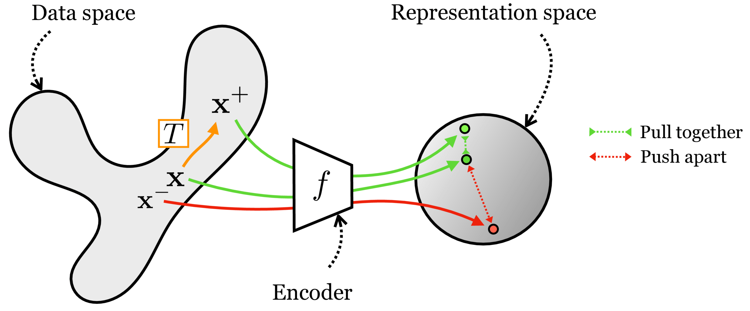
[Chen, Kornblith, Norouzi, Hinton, ICML 2020]

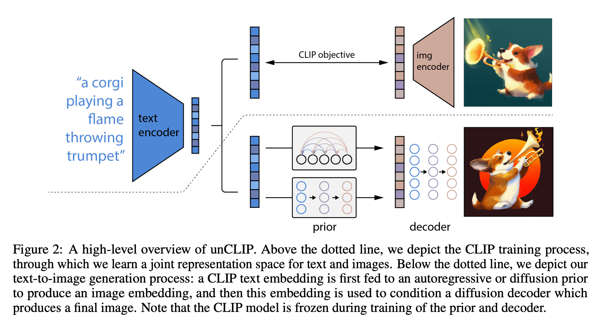
[https://arxiv.org/pdf/2204.06125.pdf]

DallE

\left) \begin{array}{l} \\ \\ \\ \\ \\ \\ \end{array} \right.

Summary

We looked at the mechanics of neural net last time. Today we see deep nets learn representations, just like our brains do.
This is useful because representations transfer — they act as prior knowledge that enables quick learning on new tasks.
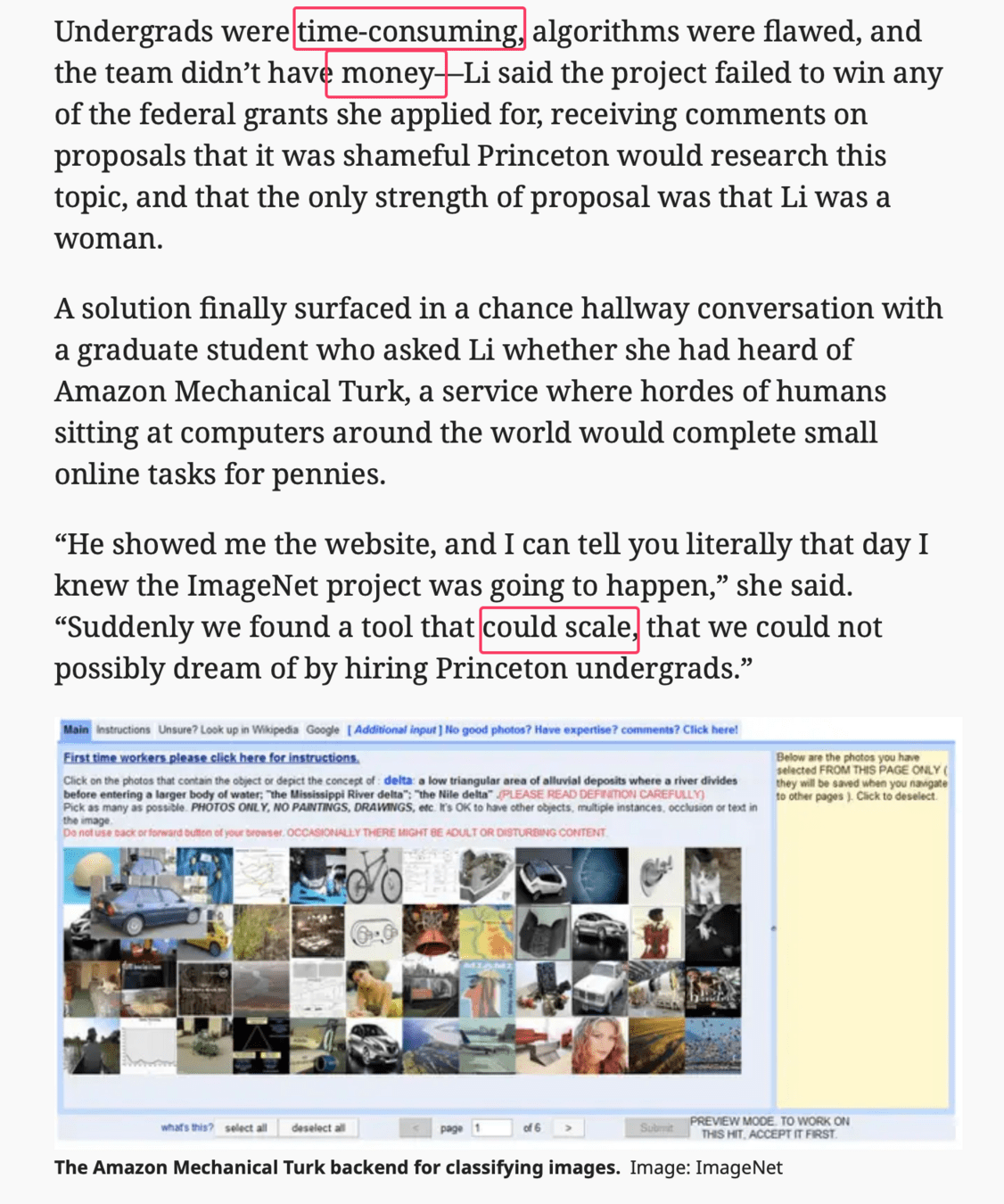
Representations can also be learned without labels, e.g. as we do in unsupervised, or self-supervised learning. This is great since labels are expensive and limiting.
Without labels there are many ways to learn representations. We saw today:
- representations as compressed codes, auto-encoder with bottleneck
- (representations that are shared across sensory modalities)
- (representations that are predictive of their context)

Thanks!

We'd love to hear your thoughts.

Lecture 7: Neural Networks II, Auto-encoders

Intro to Machine Learning

Outline

Outline

Outline

Auto-encoder

Supervised Learning

Unsupervised Learning

Training Data

Outline

Summary

Thanks!