

Lecture 3: Gradient Descent Methods
Intro to Machine Learning

Logistics
1. There is a student in our class who needs copies of class notes as an approved accommodation. If you're interested in serving as a paid note taker, please reach out to DAS, at 617-253-1674 or das-student@mit.edu.
2. Midterm 1: October 8, 730pm-9pm. It covers all the materials up to and including week 4 (linear classification). If you need to take the conflict or accommodation exam, please get in touch with us at 6.390-personal@mit.edu by Sept 24.
3. Heads-up: Midterm 2 is November 12, 730pm-9pm. Final is December 15, 9am-12pm.
More details on introML homepage
Outline
-
Gradient descent (GD)
- The gradient vector
- GD algorithm
- Gradient decent properties
- Stochastic gradient descent (SGD)
- SGD algorithm and setup
- SGD vs. GD
Recall:
- This 👉 formula is not well-defined
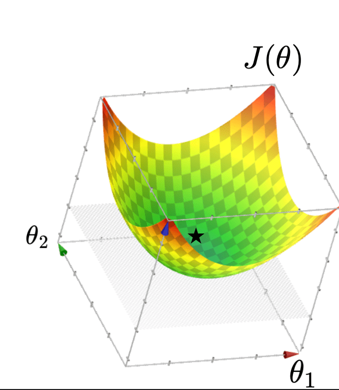
Typically, \(X\) is full column rank
- \(\theta^*=\left({X}^{\top} {X}\right)^{-1} {X}^{\top} {Y}\)
- \(J(\theta)\) "curves up" everywhere
When \(X\) is not full column rank
- \(J(\theta)\) has a "flat" bottom, like a half pipe
- Infinitely many optimal hyperplanes
- \(\theta^*\) gives the unique optimal hyperplane
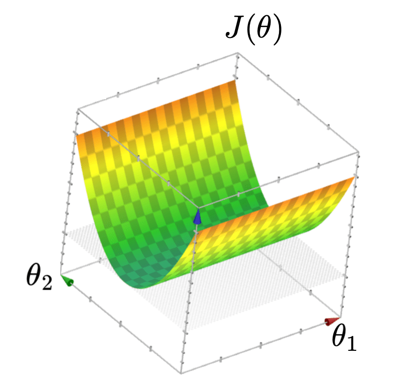
- \(\theta^*\) can be costly to compute (lab2, Q2.7)
- No way yet to obtain an optimal parameter
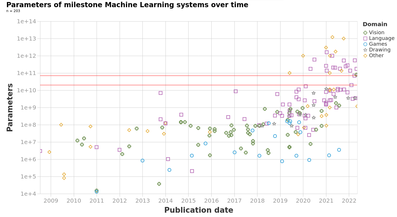
https://epoch.ai/blog/machine-learning-model-sizes-and-the-parameter-gap
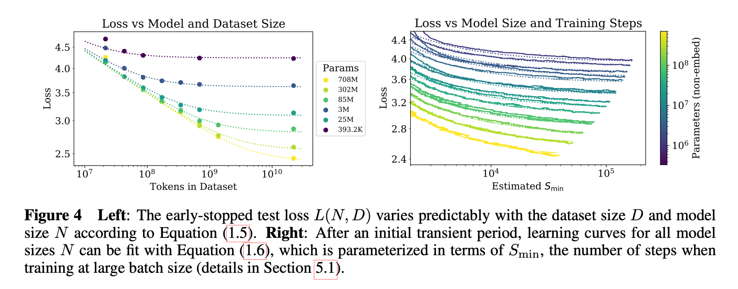
https://arxiv.org/pdf/2001.08361
In the real world,
- the number of parameters is huge
- the number of training data points is huge
- hypothesis class is typically highly nonlinear
- loss function is rarely as simple as squared error
Need a more efficient and general algorithm to train
=> gradient descent methods
Outline
-
Gradient descent algorithm (GD)
- The gradient vector
- GD algorithm
- Gradient decent properties
- Stochastic gradient descent (SGD)
- SGD algorithm and setup
- SGD vs. GD
For \(f: \mathbb{R}^m \rightarrow \mathbb{R}\), its gradient \(\nabla f: \mathbb{R}^m \rightarrow \mathbb{R}^m\) is defined at the point \(p=\left(x_1, \ldots, x_m\right)\) as:
Sometimes the gradient is undefined or ill-behaved, but today it is well-behaved.
- The gradient generalizes the concept of a derivative to multiple dimensions.
- By construction, the gradient's dimensionality always matches the function input.
3. The gradient can be symbolic or numerical.
example:
its symbolic gradient:
just like a derivative can be a function or a number.
evaluating the symbolic gradient at a point gives a numerical gradient:
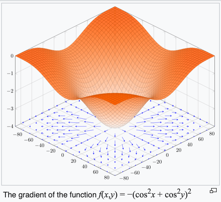
4. The gradient points in the direction of the (steepest) increase in the function value.
\(\frac{d}{dx} \cos(x) \bigg|_{x = -4} = -\sin(-4) \approx -0.7568\)
\(\frac{d}{dx} \cos(x) \bigg|_{x = 5} = -\sin(5) \approx 0.9589\)
5. The gradient at the function minimizer is necessarily zero.
For \(f: \mathbb{R}^m \rightarrow \mathbb{R}\), its gradient \(\nabla f: \mathbb{R}^m \rightarrow \mathbb{R}^m\) is defined at the point \(p=\left(x_1, \ldots, x_m\right)\) as:
Sometimes the gradient is undefined or ill-behaved, but today it is well-behaved.
- The gradient generalizes the concept of a derivative to multiple dimensions.
- By construction, the gradient's dimensionality always matches the function input.
- The gradient can be symbolic or numerical.
- The gradient points in the direction of the (steepest) increase in the function value.
- The gradient at the function minimizer is necessarily zero.
Outline
-
Gradient descent algorithm (GD)
- The gradient vector
- GD algorithm
- Gradient decent properties
- Stochastic gradient descent (SGD)
- SGD algorithm and setup
- SGD vs. GD
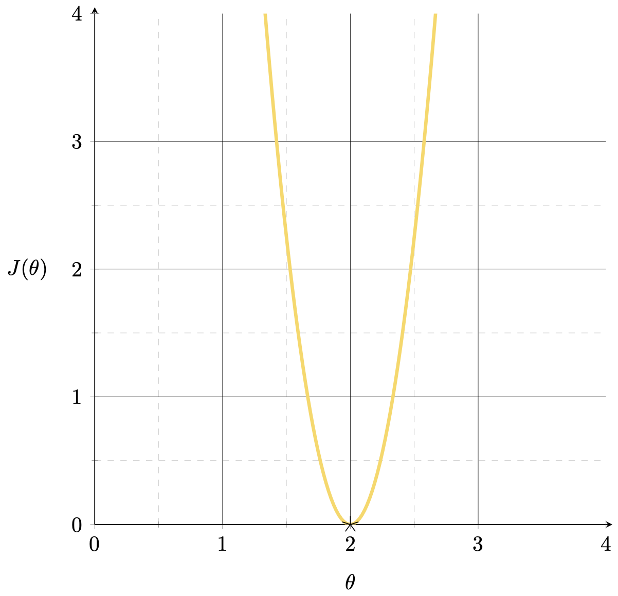
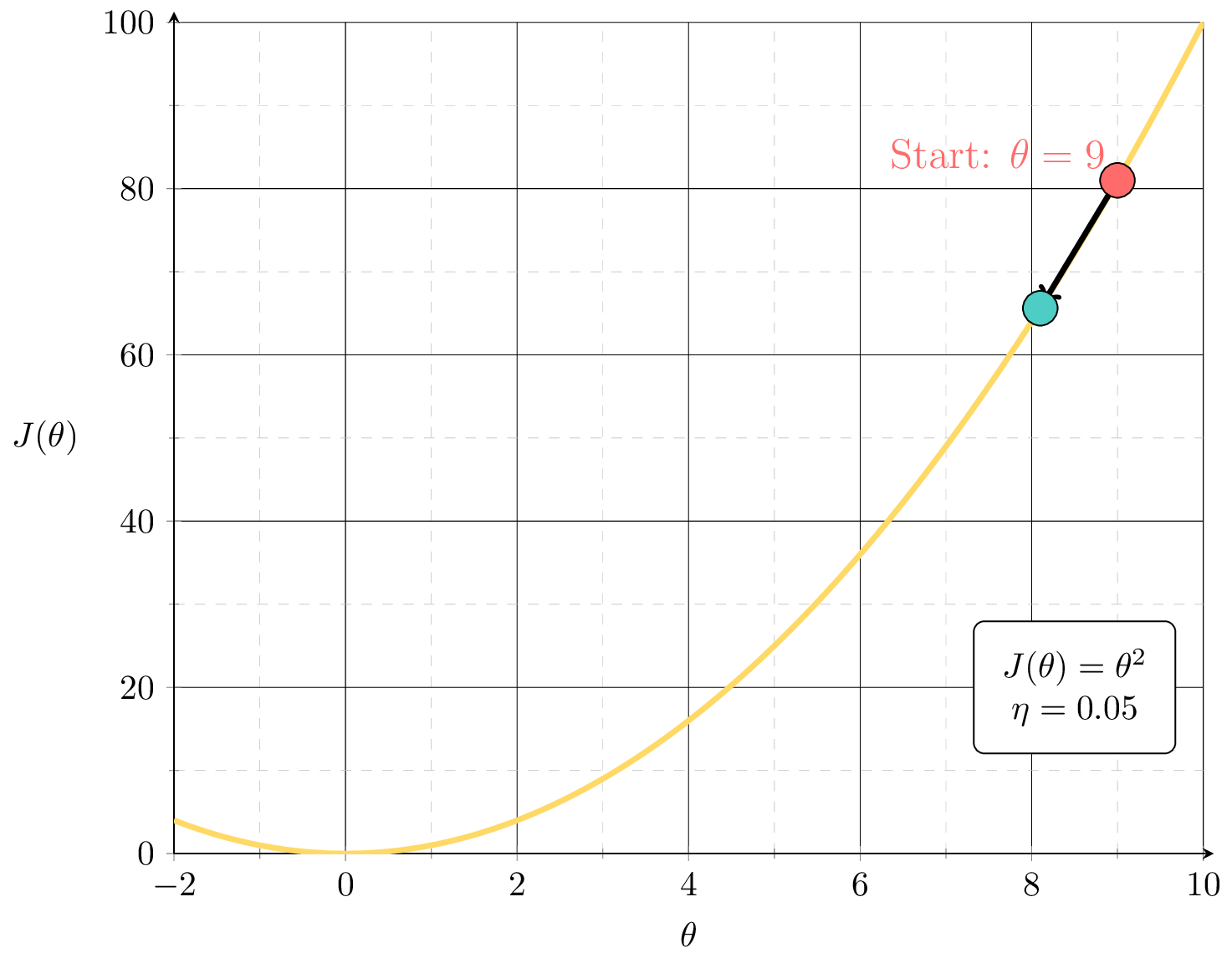
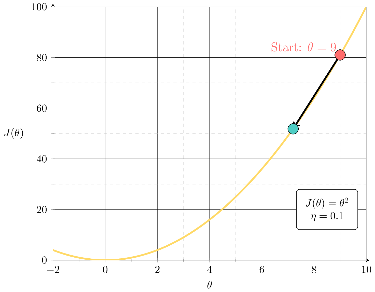
Want to fit a line (without offset) to minimize the MSE: \(J(\theta) = (3 \theta-6)^{2}\)
A single training data point
\((x,y) = (3,6)\)
MSE could get better.
How to formalize this?
Suppose we fit a line \(y= 1.5x\)
1.5
\(\nabla_\theta J = J'(\theta) \)
\(J(\theta) = (3 \theta-6)^{2}\)
\( = 2[3(3 \theta-6)]|_{\theta=1.5}\)
\(<0\)
MSE could get better. How to?
Leveraging the gradient.
Suppose we fit a line \(y= 1.5x\)
1.5
\( = 2[3(3 \theta-6)]|_{\theta=2.4}\)
\(>0\)
MSE could get better. How to?
Leveraging the gradient.
Suppose we fit a line \(y= 2.4 x\)
\(\nabla_\theta J = J'(\theta) \)
\(J(\theta) = (3 \theta-6)^{2}\)
2.4
hyperparameters
initial guess
of parameters
learning rate
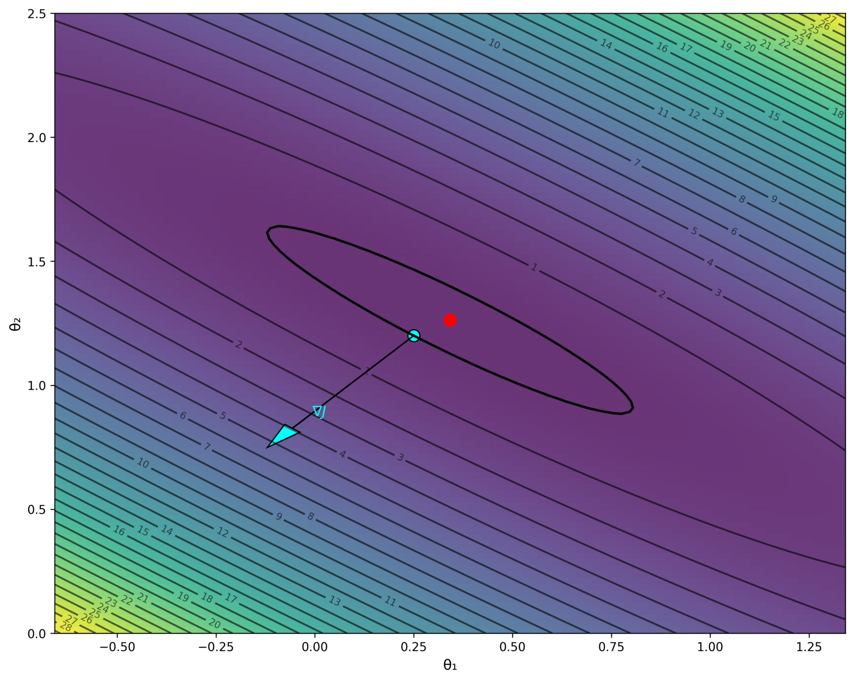
precision
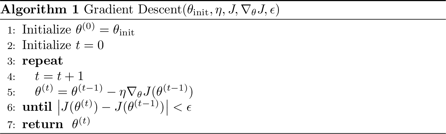
level set,
contour plot

iteration counter
- What does this 2d vector represent? anything in the psuedocode?
- What does this 3d vector represent? anything in the psuedocode?
objective improvement is nearly zero.
Other possible stopping criterion for line 6:
- Small parameter change: \( \|\theta^{(t)} - \theta^{(t-1)}\| < \epsilon \), or
- Small gradient norm: \( \|\nabla_{\theta} J(\theta^{(t-1)})\| < \epsilon \)
Outline
-
Gradient descent algorithm (GD)
- The gradient vector
- GD algorithm
- Gradient decent properties
- Stochastic gradient descent (SGD)
- SGD algorithm and setup
- SGD vs. GD

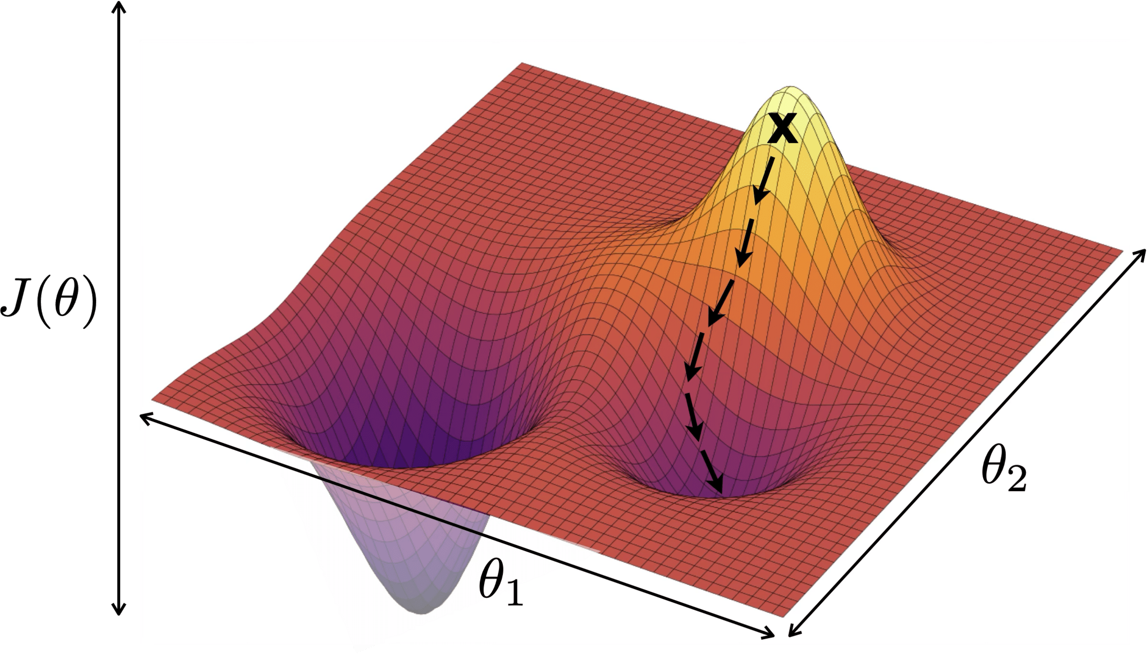
When minimizing a function, we aim for a global minimizer.


At a global minimizer
the gradient vector is zero
\(\Rightarrow\)
\(\nLeftarrow\)

gradient descent can achieve this (to arbitrary precision)
the gradient vector is zero
\(\Leftarrow\)
the objective function is convex
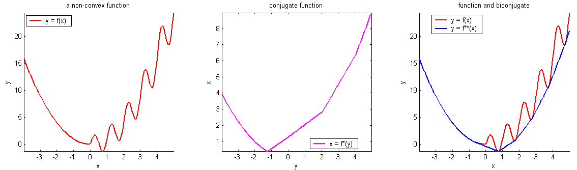
A function \(f\) is convex if any line segment connecting two points of the graph of \(f\) lies above or on the graph.
- \(f\) is concave if \(-f\) is convex.
- Convex functions are the largest well-understood class of functions where optimization theory guarantees convergence and efficiency
When minimizing a function, we aim for a global minimizer.
At a global minimizer
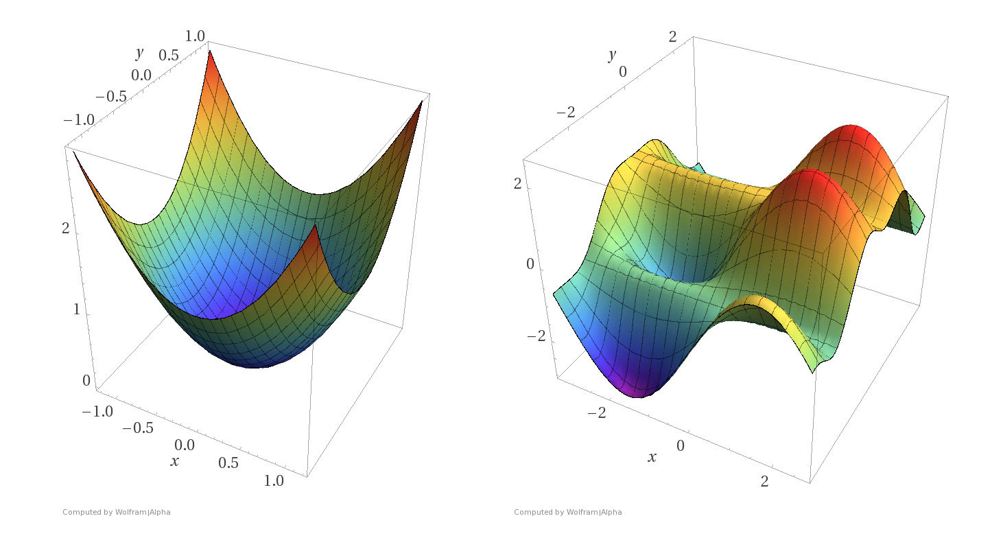
Some examples
Convex functions
Non-convex functions


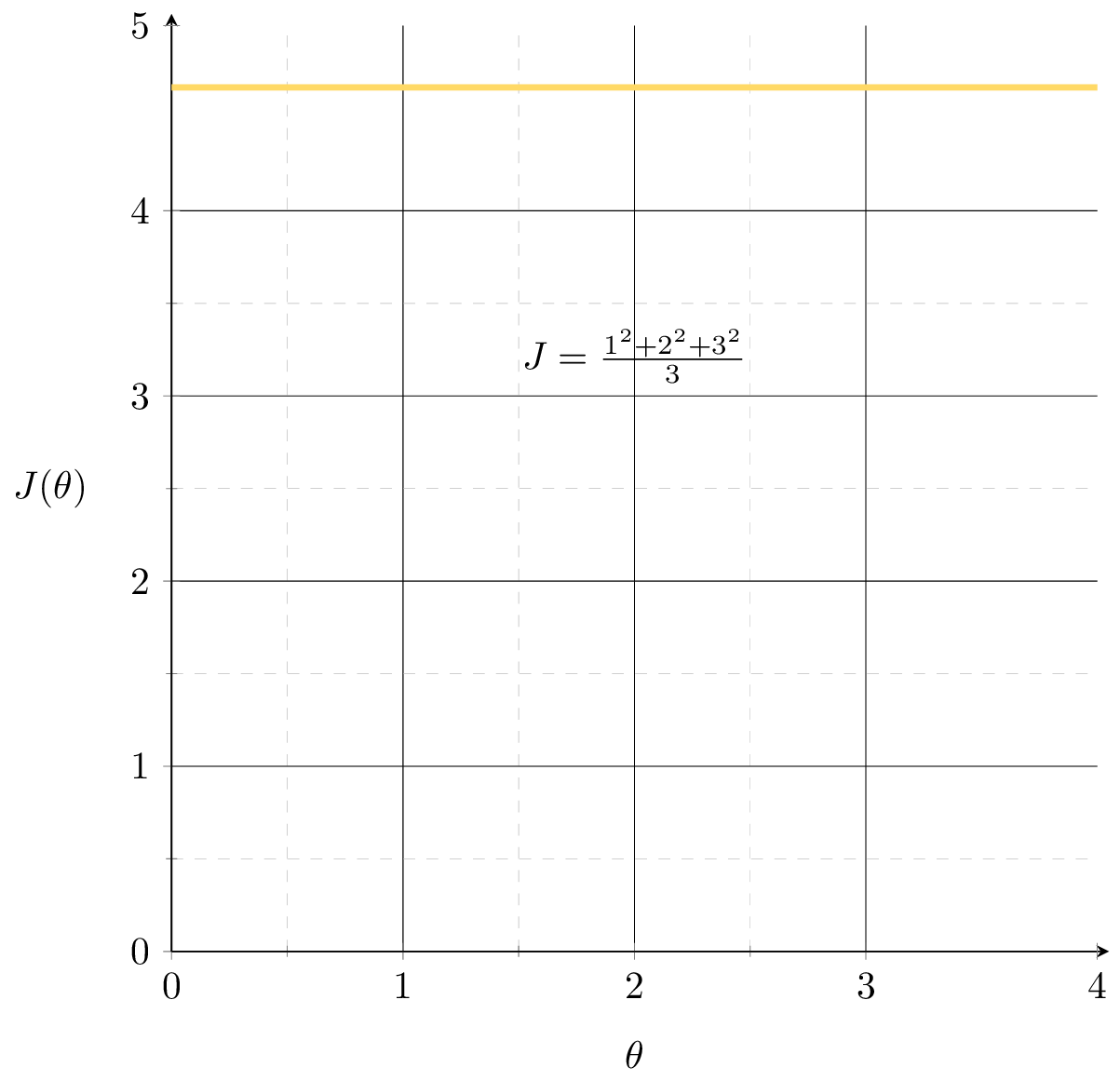
- MSE: \( J(\theta) =\frac{1}{n}({X} \theta-{Y})^{\top}({X} \theta-{Y})\)
convexity is why we can claim the point whose gradient is zero is a global minimizer.
is always convex

\((x_1, x_2) = (2,3), y =7\)
\((x_1, x_2) = (4,6), y =8\)
\((x_1, x_2) = (6,9), y =9\)
case (c) training data set again
- Ridge objective with \(\lambda >0\) is always (strongly) convex
convexity is why we can claim the point whose gradient is zero is a global minimizer.
- Assumptions:
- \(f\) is sufficiently "smooth"
- \(f\) is convex
- \(f\) has at least one global minimum
- Run gradient descent for sufficient iterations
- \(\eta\) is sufficiently small
- Conclusion:
- Gradient descent converges arbitrarily close to a global minimizer of \(f\).
Gradient Descent Performance
if violated, may not have gradient,
can't run gradient descent
Gradient Descent Performance
- Assumptions:
- \(f\) is sufficiently "smooth"
- \(f\) is convex
- \(f\) has at least one global minimum
- Run gradient descent for sufficient iterations
- \(\eta\) is sufficiently small
- Conclusion:
- Gradient descent converges arbitrarily close to a global minimizer of \(f\).
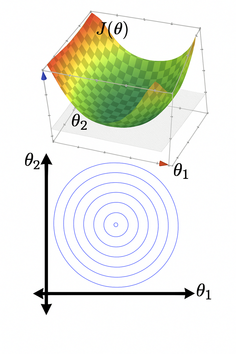
if violated, may get stuck at a saddle point
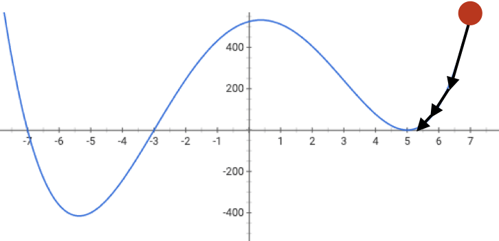
or a local minimum
- Assumptions:
- \(f\) is sufficiently "smooth"
- \(f\) is convex
- \(f\) has at least one global minimum
- Run gradient descent for sufficient iterations
- \(\eta\) is sufficiently small
- Conclusion:
- Gradient descent converges arbitrarily close to a global minimizer of \(f\).
Gradient Descent Performance
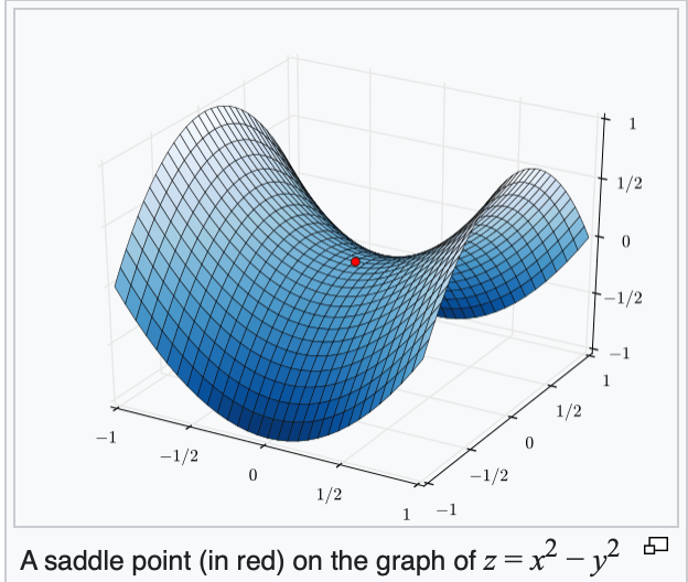
if violated:
may not terminate/no minimum to converge to

Gradient Descent Performance
- Assumptions:
- \(f\) is sufficiently "smooth"
- \(f\) is convex
- \(f\) has at least one global minimum
- Run gradient descent for sufficient iterations
- \(\eta\) is sufficiently small
- Conclusion:
- Gradient descent converges arbitrarily close to a global minimizer of \(f\).
Gradient Descent Performance
- Assumptions:
- \(f\) is sufficiently "smooth"
- \(f\) is convex
- \(f\) has at least one global minimum
- Run gradient descent for sufficient iterations
- \(\eta\) is sufficiently small
- Conclusion:
- Gradient descent converges arbitrarily close to a global minimizer of \(f\).
if violated:
see demo on next slide, also lab/hw

Outline
- Gradient descent algorithm (GD)
- The gradient vector
- GD algorithm
- Gradient decent properties
-
Stochastic gradient descent (SGD)
- SGD algorithm and setup
- SGD vs. GD
Fit a line (without offset) to the dataset, the MSE:
training data

| p1 | 2 | 5 |
| p2 | 3 | 6 |
| p3 | 4 | 7 |

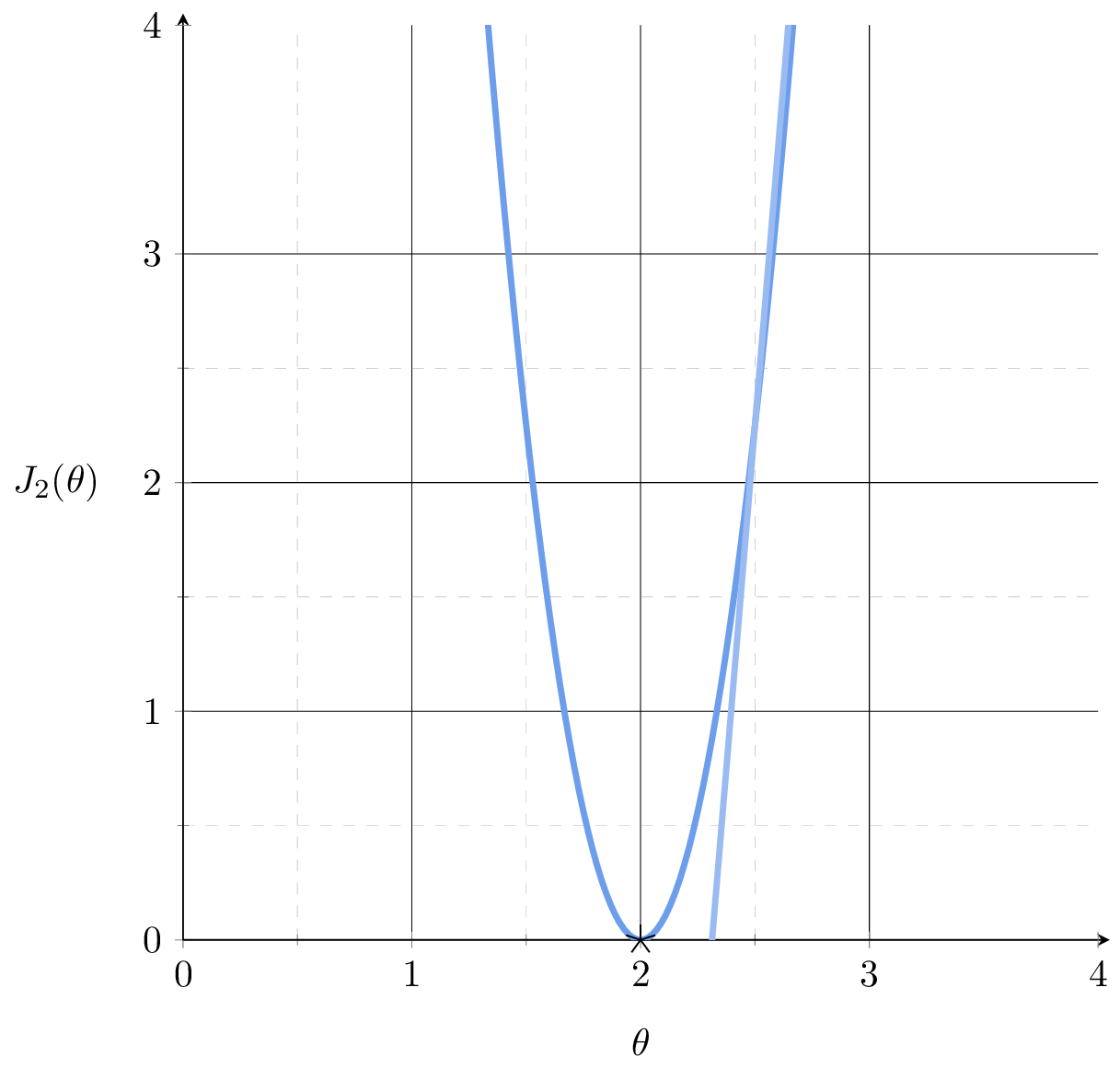
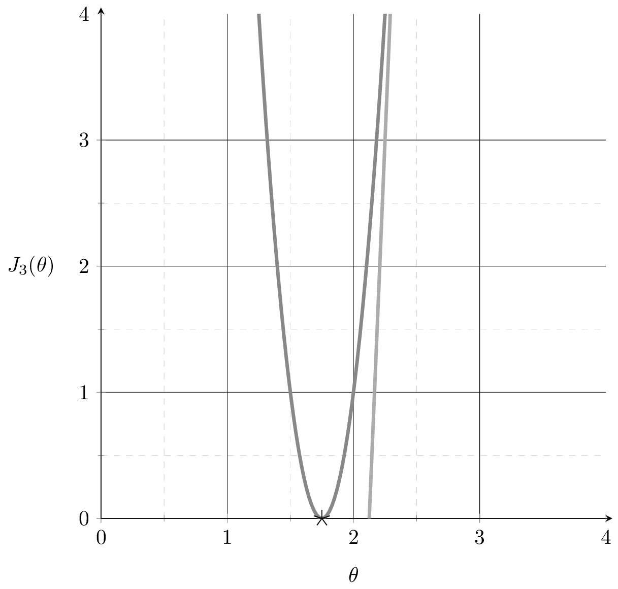
\(J(\theta) = \frac{1}{3}\left[(2 \theta-5)^2+(3 \theta-6)^{2}+(4 \theta-7)^2\right]\)
Suppose we fit a line \(y= 2.5x\)
\(J(\theta) = \frac{1}{3}\left[(2 \theta-5)^2+(3 \theta-6)^{2}+(4 \theta-7)^2\right]\)
\(\nabla_\theta J = \frac{1}{3}[4(2 \theta-5)+6(3 \theta-6)+8(4 \theta-7)]|_{\theta=2.5}\)
gradient info can help MSE get better
\(= \frac{1}{3}[0+6(7.5-6)+8(10-7)] = 11\)
11
2.5
\(J(\theta) = \frac{1}{3}\left[(2 \theta-5)^2+(3 \theta-6)^{2}+(4 \theta-7)^2\right]\)
- the MSE of a linear hypothesis:
\(\nabla_\theta J = \frac{1}{3}[4(2 \theta-5)+6(3 \theta-6)+8(4 \theta-7)]\)
- and its gradient w.r.t. \(\theta\):
\( = \frac{1}{3}\left[ \quad \quad \right]\)
\( J_1\)
\( J_2\)
\( J_3\)
\( +\)
\( +\)
\( = \frac{1}{3}\left[ \quad \quad \quad \quad \right]\)
\(\nabla_\theta J_1\)
\(\nabla_\theta J_2\)
\( \nabla_\theta J_3\)
\( +\)
\( +\)
| p1 | 2 | 5 |
| p2 | 3 | 6 |
| p3 | 4 | 7 |
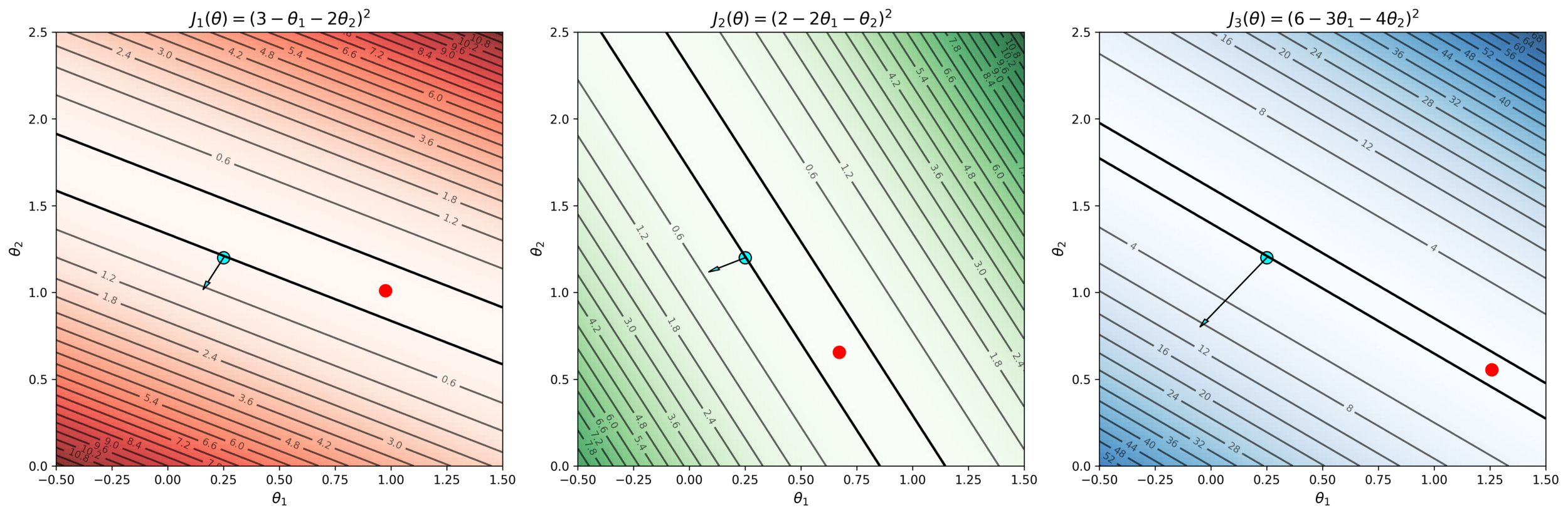
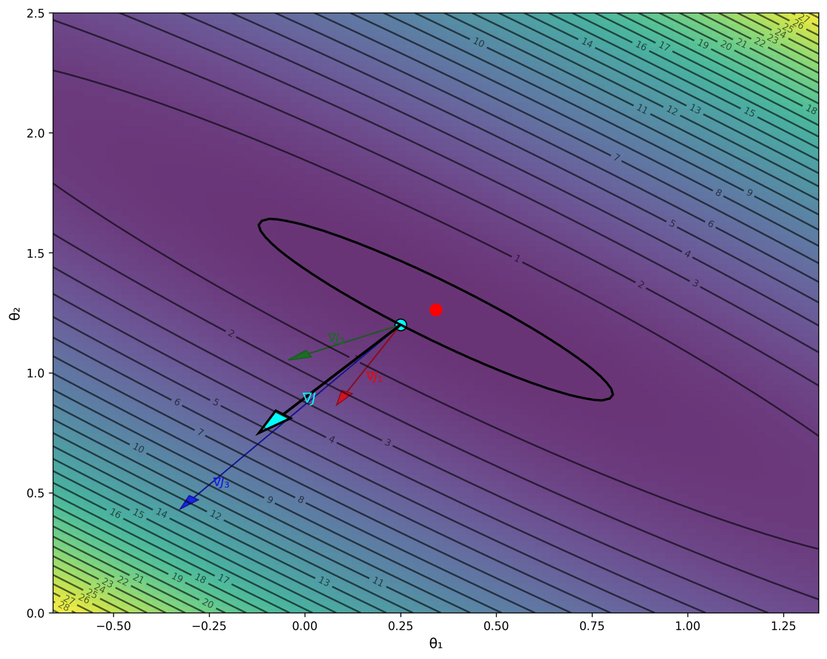
Gradient of an ML objective
- the MSE of a linear hypothesis:
- and its gradient w.r.t. \(\theta\):
Using our example data set,
\(J(\theta) = \frac{1}{3}\left[(2 \theta-5)^2+(3 \theta-6)^{2}+(4 \theta-7)^2\right]\)
- the MSE of a linear hypothesis:
\(\nabla_\theta J = \frac{1}{3}[4(2 \theta-5)+6(3 \theta-6)+8(4 \theta-7)]\)
- and its gradient w.r.t. \(\theta\):
Using any dataset,
Gradient of an ML objective
- An ML objective function is a finite sum
- and its gradient w.r.t. \(\theta\):
In general,
👋 (gradient of the sum) = (sum of the gradient)
👆
- the MSE of a linear hypothesis:
- and its gradient w.r.t. \(\theta\):
Gradient of an ML objective
- An ML objective function is a finite sum
- and its gradient w.r.t. \(\theta\):
In general,
gradient info from a single \(i^{\text{th}}\) data point's loss
need to add \(n\) of these, each\(\nabla_\theta J_i(\theta) \in \mathbb{R}^{d}\)
Costly in practice!
loss incurred on a single \(i^{\text{th}}\) data point
\(J(\theta) = \frac{1}{3}\left[(2 \theta-5)^2+(3 \theta-6)^{2}+(4 \theta-7)^2\right]\)
- the MSE of a linear hypothesis:
\(\nabla_\theta J = \frac{1}{3}[4(2 \theta-5)+6(3 \theta-6)+8(4 \theta-7)]\)
- and its gradient w.r.t. \(\theta\):
\( = \frac{1}{3}\left[ \quad \quad \right]\)
\( J_1\)
\( J_2\)
\( J_3\)
\( +\)
\( +\)
\( = \frac{1}{3}\left[ \quad \quad \quad \quad \right]\)
\(\nabla_\theta J_1\)
\(\nabla_\theta J_2\)
\( \nabla_\theta J_3\)
\( +\)
\( +\)
| p1 | 2 | 5 |
| p2 | 3 | 6 |
| p3 | 4 | 7 |
| p1 | 2 | 5 |
| p2 | 3 | 6 |
| p3 | 4 | 7 |
| x1 | x2 | y | |
|---|---|---|---|
| p1 | 1 | 2 | 3 |
| p2 | 2 | 1 | 2 |
| p3 | 3 | 4 | 6 |
| x1 | x2 | y | |
|---|---|---|---|
| p1 | 1 | 2 | 3 |
| p2 | 2 | 1 | 2 |
| p3 | 3 | 4 | 6 |
| x1 | x2 | y | |
|---|---|---|---|
| p1 | 1 | 2 | 3 |
| p2 | 2 | 1 | 2 |
| p3 | 3 | 4 | 6 |
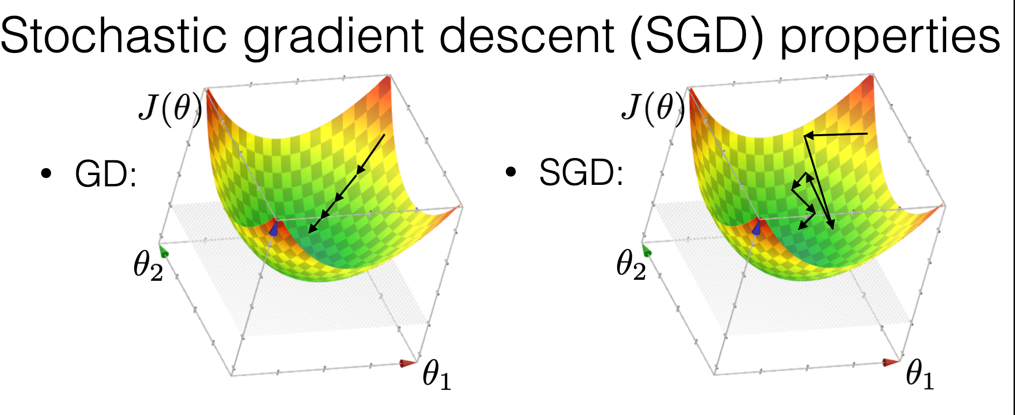
is much more "random"
is more efficient
may get us out of a local min

Compared with GD, SGD:
Stochastic gradient descent performance
\(\sum_{t=1}^{\infty} \eta(t)=\infty\) and \(\sum_{t=1}^{\infty} \eta(t)^2<\infty\)
- Assumptions:
- \(f\) is sufficiently "smooth"
- \(f\) is convex
- \(f\) has at least one global minimum
- Run gradient descent for sufficient iterations
- \(\eta\) is sufficiently small and satisfies additional "scheduling" condition
- Conclusion:
- Stochastic gradient descent converges arbitrarily close to a global minimum of \(f\) with probability 1.
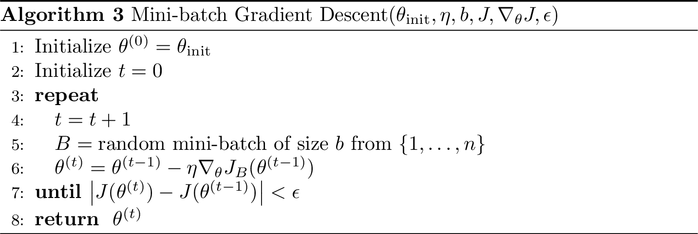
batch size
🥰more accurate gradient estimate
🥰stronger theoretical guarantee
🥺higher cost per parameter update
mini-batch GD
SGD
GD
Summary
-
Most ML methods can be formulated as optimization problems. We won’t always be able to solve optimization problems analytically (in closed-form) nor efficiently.
-
We can still use numerical algorithms to good effect. Lots of sophisticated ones available. Gradient descent is one of the simplest.
-
The GD algorithm, iterative algorithm, keeps applying the parameter update rule.
-
Under appropriate conditions (most notably, when objective function is convex, and when learning rate is small enough), GD can guarantee convergence to a global minimum.
-
SGD is approximated GD, it uses a single data point to approximate the entire data set, it's more efficient, more random, and less guarantees.
-
mini-batch GD is a middle ground between GD and SGD.
Thanks!
We'd love to hear your thoughts.
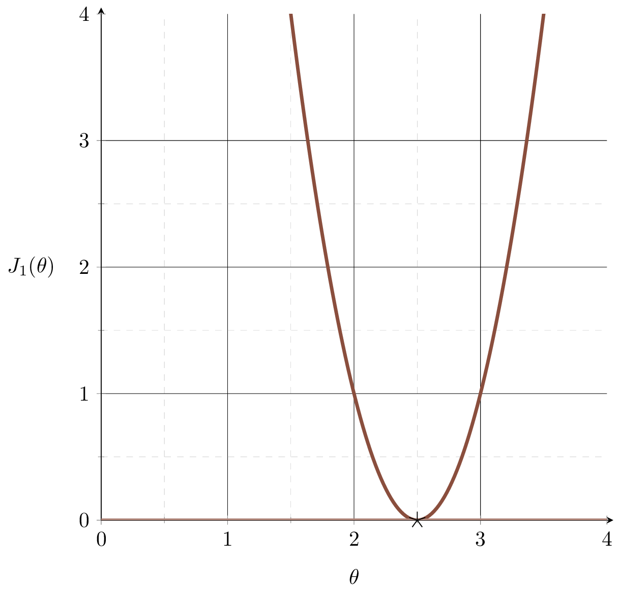
- A function \(f\) on \(\mathbb{R}^m\) is convex if any line segment connecting two points of the graph of \(f\) lies above or on the graph.
- For convex functions, all local minima are global minima.
What do we need to know:
- Intuitive understanding of the definition
- If given a function, can determine if it's convex. (We'll only ever give at most 2-dimensional input, these are "easy" cases where visual understanding suffices)
- Understand how gradient descent algorithms may fail without convexity.
- Recognize that OLS loss function is convex, ridge regression loss is (strictly) convex, and later cross-entropy loss function is convex too.
\(J(\theta) = \frac{1}{3}\left[(2 \theta-5)^2+(3 \theta-6)^{2}+(4 \theta-7)^2\right]\)
\(\nabla_\theta J = \frac{1}{3}[4(2 \theta-5)+6(3 \theta-6)+8(4 \theta-7)]\)
- the MSE of a linear hypothesis:
- and its gradient w.r.t. \(\theta\):
| p1 | 2 | 5 |
| p2 | 3 | 6 |
| p3 | 4 | 7 |