\boxed{h}

Regression

Algorithm

\rightarrow

\(\mathcal{D}_\text{train}\)

\rightarrow

🧠⚙️

hypothesis class

loss function

hyperparameters

Recap:

regressor

\in \mathbb{R}^d

\in \mathbb{R}

y

\downarrow

"Use" a model

"Learn" a model

\rightarrow

\downarrow

x

\downarrow

Recap:

"Use" a model

"Learn" a model

\rightarrow

\downarrow

train, optimize, tune, adapt ...

adjusting/updating/finding \(\theta\)

gradient based

\boxed{h}

Regression

Algorithm

\rightarrow

\(\mathcal{D}_\text{train}\)

\rightarrow

🧠⚙️

hypothesis class
loss function
hyperparameters

regressor

\in \mathbb{R}^d

\in \mathbb{R}

y

\downarrow

x

predict, test, evaluate, infer ...

plug in the \(\theta\) found

no gradients involved

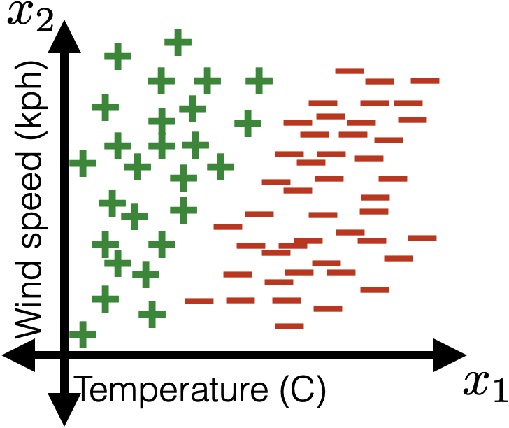
Classification

Algorithm

🧠⚙️
hypothesis class
loss function
hyperparameters

Today:

classifier

\in \mathbb{R}^d

\in \text{a discrete set}

\downarrow

x

y

\downarrow

\rightarrow

\boxed{h}

\(\mathcal{D}_\text{train}\)

\rightarrow

{"good", "better", "best", ...}

\(\{+1,0\}\)

\(\{😍, 🥺\}\)

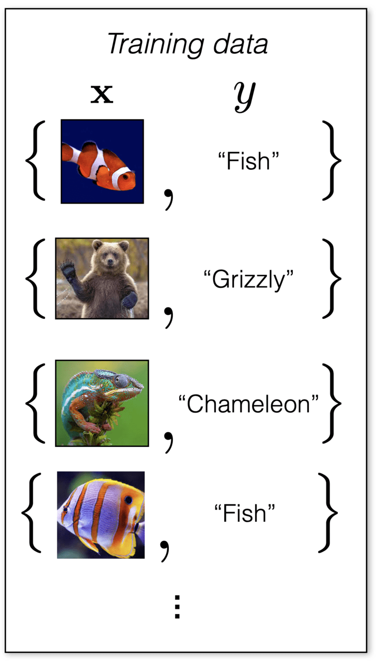
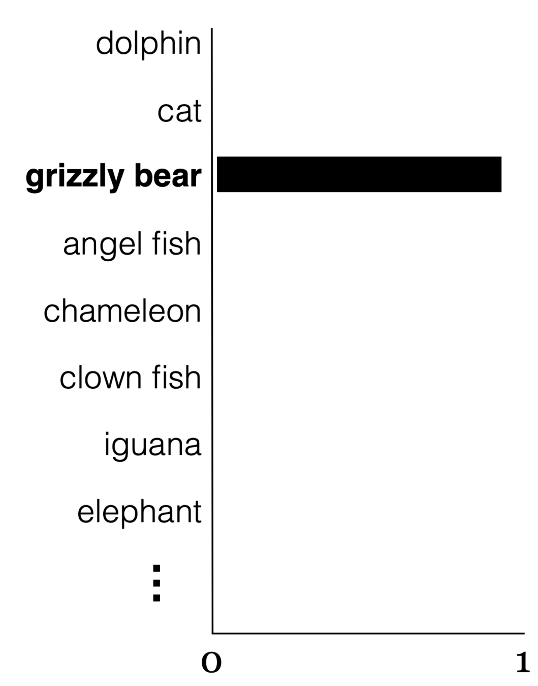
{"Fish", "Grizzly", "Chameleon", ...}

Classification

Algorithm

🧠⚙️
hypothesis class
loss function
hyperparameters

classifier

\in

\downarrow

x

y

\downarrow

\rightarrow

\boxed{h}

\rightarrow

{"Fish", "Grizzly", "Chameleon", ...}

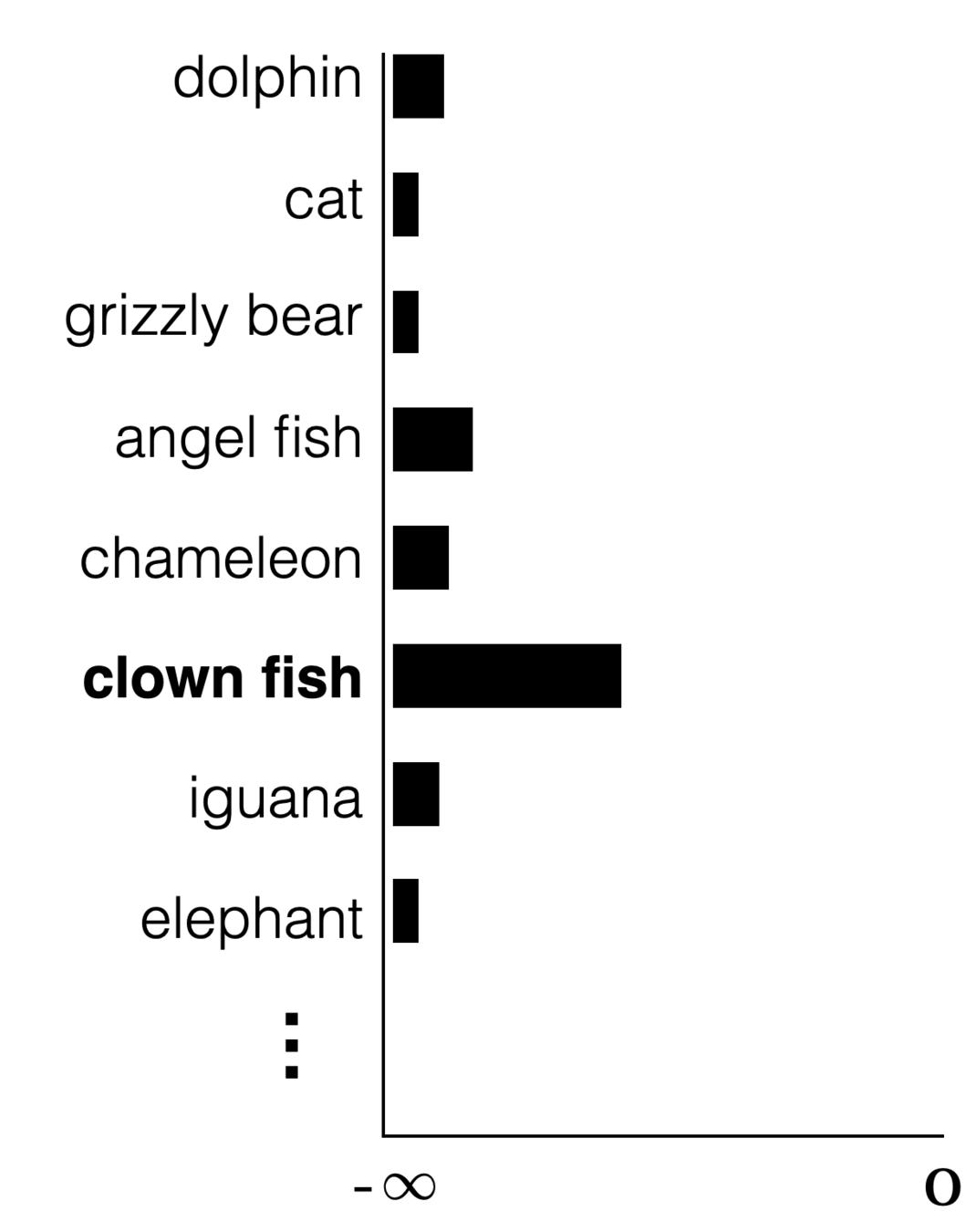
"Fish"

images adapted from Phillip Isola

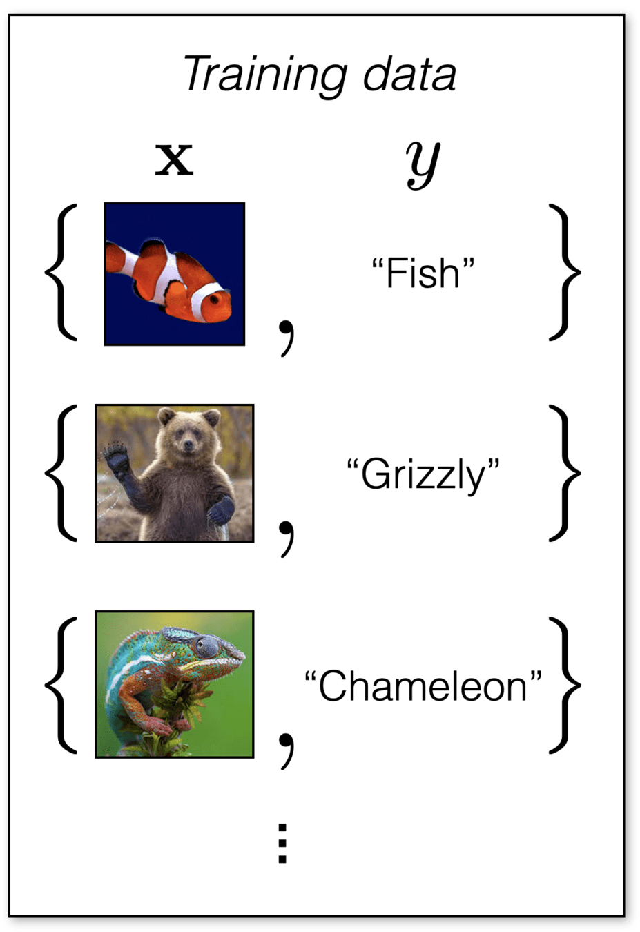
features

label

\in \text{a discrete set}

Outline

Linear (binary) classifiers
- to use: separator, normal vector
- to learn: difficult! won't do
Linear logistic (binary) classifiers
- to use: sigmoid
- to learn: negative log-likelihood loss
Linear multi-class classifiers
- to use: softmax
- to learn: one-hot encoding, cross-entropy loss

linear regressor

linear binary classifier

features

parameters

linear combination

predict

\(x \in \mathbb{R}^d\)

\(\theta \in \mathbb{R}^d, \theta_0 \in \mathbb{R}\)

\(\theta^T x +\theta_0\)

\(g = z\)

\(=z\)

if \(z > 0\)

otherwise

\left\{ \begin{array}{l} \\ \\ \end{array} \right.

\(1\)

0

today, we refer to \(\theta^T x +\theta_0\) as \(z\) throughout.

\(g=\)

label

\(y\in \mathbb{R}\)

\(y\in \{0,1\}\)

Outline

Linear (binary) classifiers
- to use: separator, normal vector
- to learn: difficult! won't do
Linear logistic (binary) classifiers
- to use: sigmoid
- to learn: negative log-likelihood loss
Multi-class classifiers
- to use: softmax
- to learn: one-hot encoding, cross-entropy loss

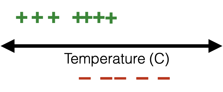
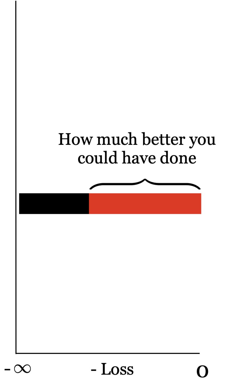
\mathcal{L}_{01}(g, y)=\left\{\begin{array}{ll} 0 & \text { if } \text{guess} = \text{label} \\ 1 & \text { otherwise } \end{array}\right .

To learn a model, need a loss function.

g = \operatorname{step}\left(z\right) = \operatorname{step}\left(\theta^{\top} x+\theta_0\right)

Very intuitive, and easy to evaluate 😍

One natural loss choice:

y

\mathcal{L}_{01}(g, a) = 0

\mathcal{L}_{01}(g, a) = 1

Very hard to optimize (NP-hard) 🥺

"Flat" almost everywhere (zero gradient)
"Jumps" elsewhere (no gradient)

linear binary classifier

features

parameters

linear combo

predict

\(x \in \mathbb{R}^d\)

\(\theta \in \mathbb{R}^d, \theta_0 \in \mathbb{R}\)

\(\theta^T x +\theta_0\)

\(=z\)

loss

\((g - y)^2 \)

\left\{\begin{array}{ll} 0 & \text { if } g = y \\ 1 & \text { otherwise } \end{array}\right .

g = z

linear regressor

closed-form or

gradient descent

NP-hard to learn

optimize via

if \(z > 0\)

otherwise

\left\{ \begin{array}{l} \\ \\ \end{array} \right.

\(1\)

0

\(g=\)

\(y \in \mathbb{R}\)

\(y \in \{0,1\}\)

both discrete

Outline

Linear (binary) classifiers
- to use: separator, normal vector
- to learn: difficult! won't do
Linear logistic (binary) classifiers
- to use: sigmoid
- to learn: negative log-likelihood loss
Linear multi-class classifiers
- to use: softmax
- to learn: one-hot encoding, cross-entropy loss

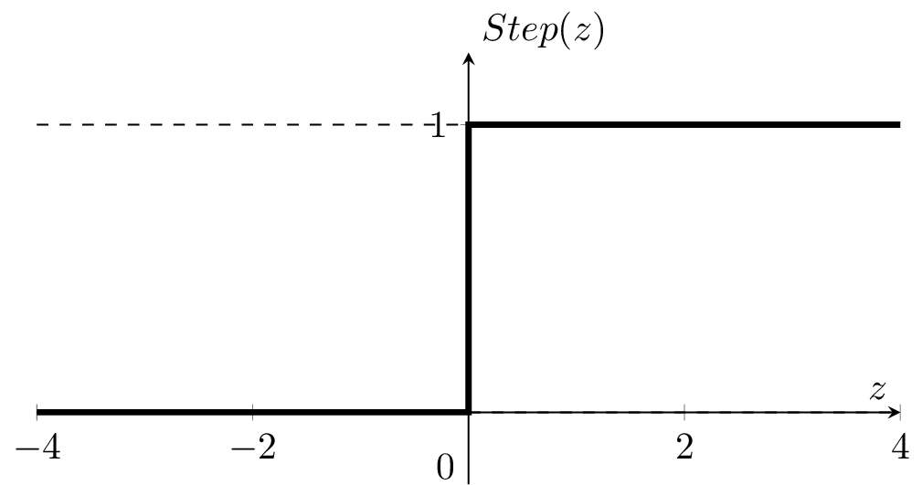
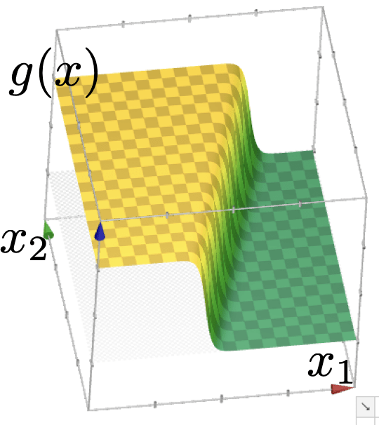
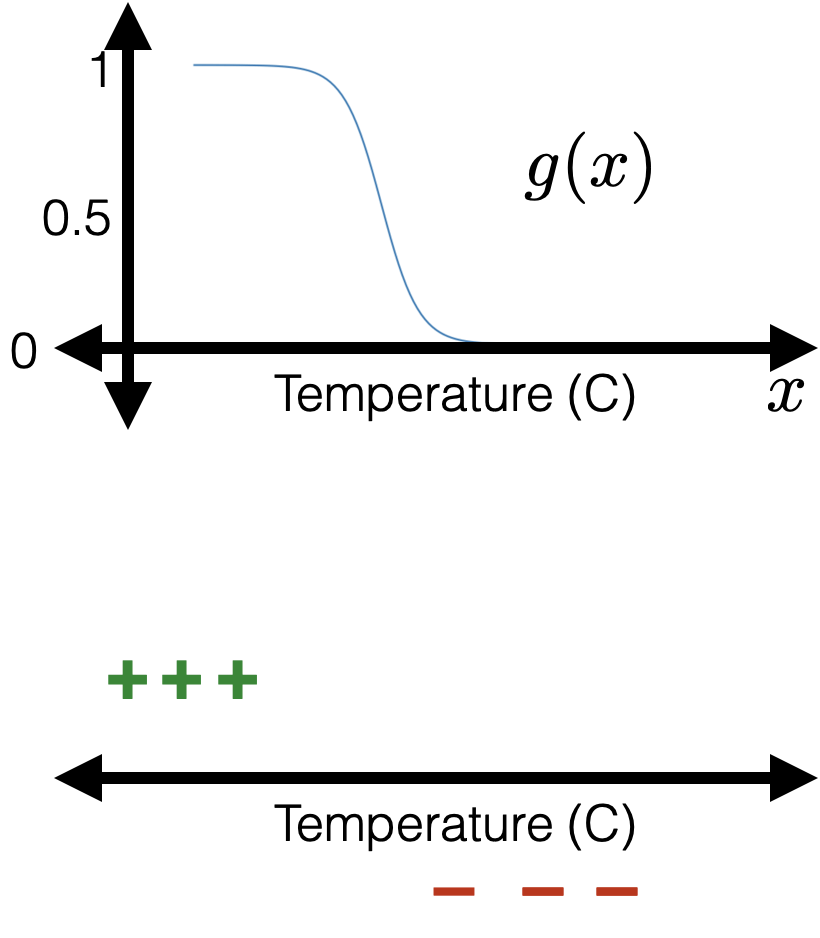
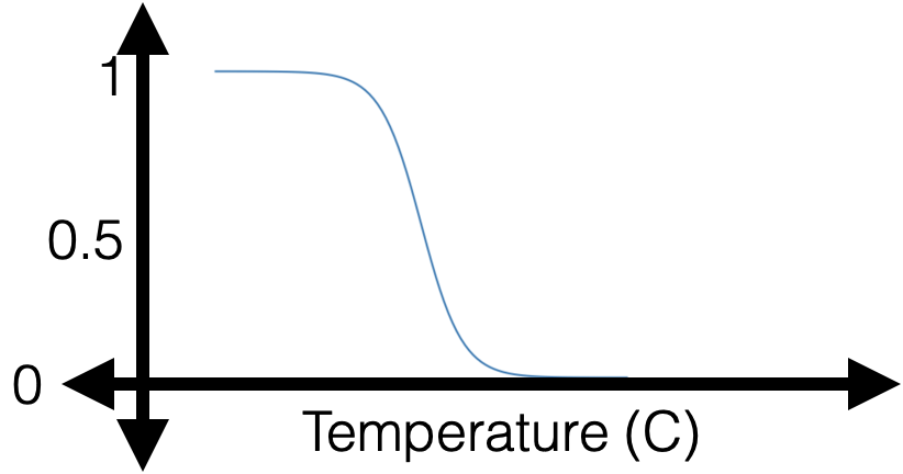
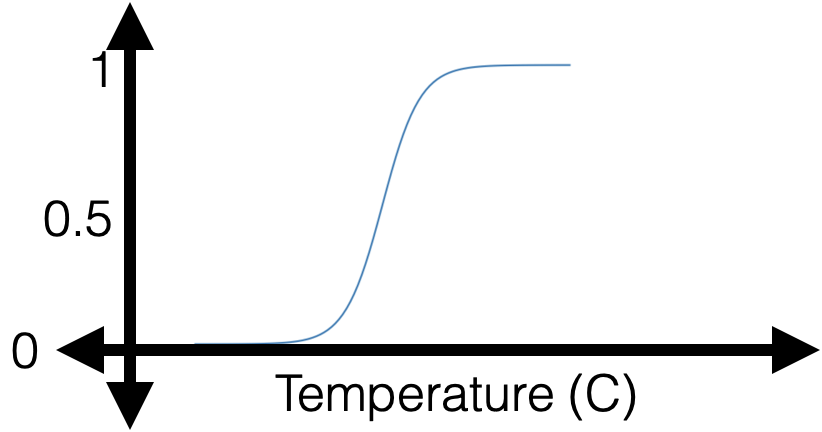
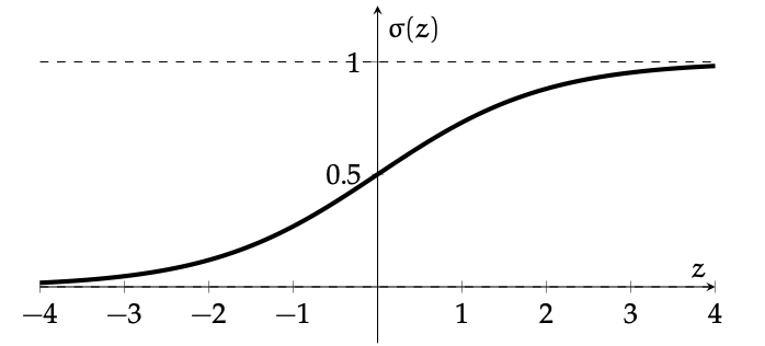
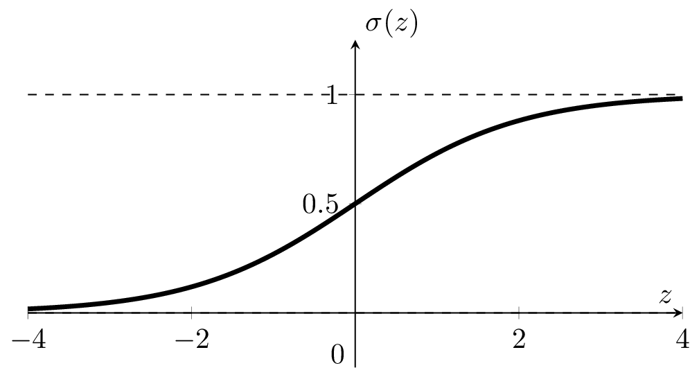
: a smooth step function

:= \frac{1}{1+e^{-z}}

Sigmoid

if \(z > 0\)

otherwise

\left\{ \begin{array}{l} \\ \\ \end{array} \right.

\(1\)

0

if \(\sigma(z) > 0.5\)

otherwise

\left\{ \begin{array}{l} \\ \\ \end{array} \right.

\(1\)

0

Predict

\(z\) is called the logit

linear binary classifier

features

parameters

linear combo

predict

\(x \in \mathbb{R}^d\)

\(\theta \in \mathbb{R}^d, \theta_0 \in \mathbb{R}\)

\(\theta^T x +\theta_0\)

\(=z\)

linear logistic binary classifier

if \(z > 0\)

otherwise

\left\{ \begin{array}{l} \\ \\ \end{array} \right.

\(1\)

0

if \(\sigma(z) > 0.5\)

otherwise

\left\{ \begin{array}{l} \\ \\ \end{array} \right.

\(1\)

0

:= \frac{1}{1+e^{-z}}

features

parameters

linear combo

predict

\(x \in \mathbb{R}^d\)

\(\theta \in \mathbb{R}^d, \theta_0 \in \mathbb{R}\)

\(\theta^T x +\theta_0\)

\(=z\)

linear logistic binary classifier

if \(\sigma(z) > 0.5\)

otherwise

\left\{ \begin{array}{l} \\ \\ \end{array} \right.

\(1\)

0

Sigmoid squashes the logit \(z\) into a number in \((0, 1)\).

= \frac{1}{1+e^{-\left(\theta^{\top} x+\theta_0\right)}}

if \(\sigma(z) \)

> 0.5

Predict positive class label 1

= \frac{1}{1+e^{-z}}

The logit \(z\) is a linear combo of \(x\) via the parametes.

\(\sigma\left(\cdot\right):\) the model's confidence or estimated likelihood that feature \(x\) belongs to the positive class.

\(\theta\), \(\theta_0\) can flip, squeeze, expand, or shift the \(\sigma\left(x\right)\) graph horizontally
\(\sigma\left(\cdot\right)\) monotonic, very elegant gradient (see hw/lab)

images credit: Tamara Broderick

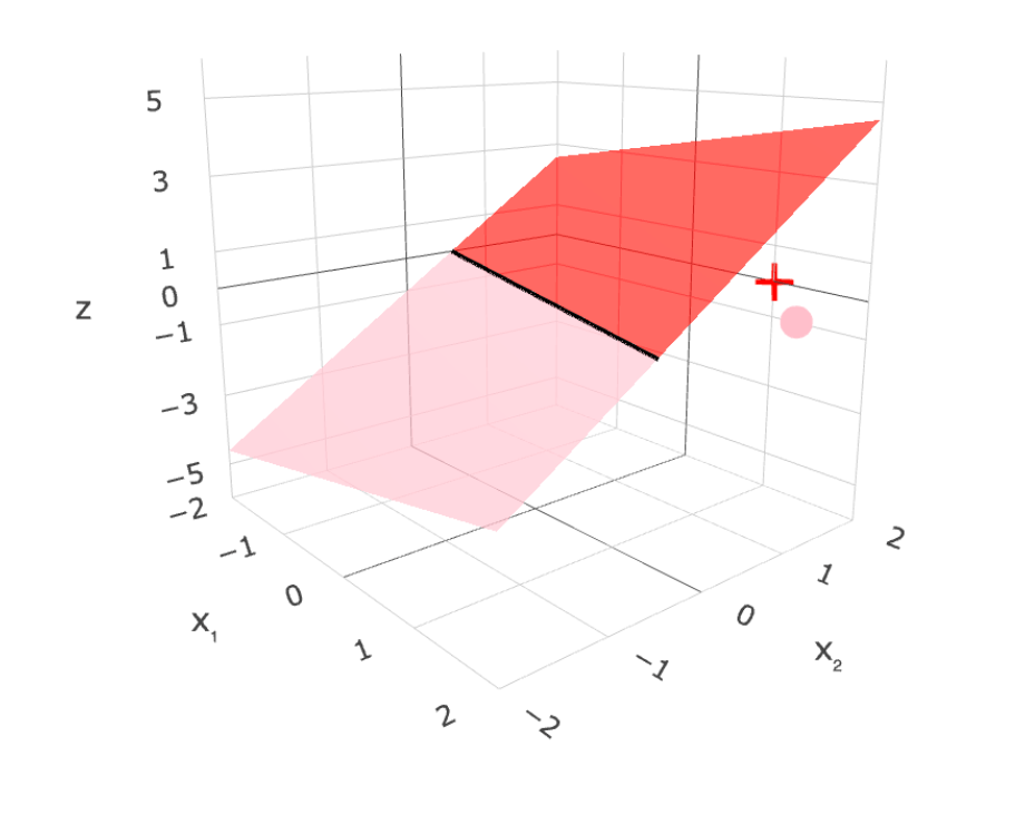
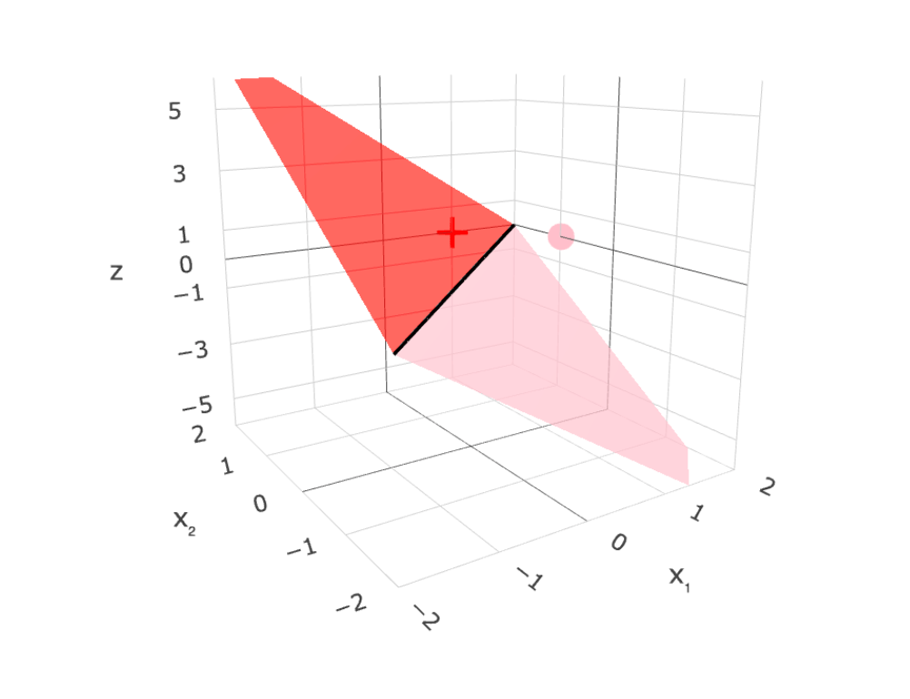
linear separator

\(z = \theta^T x+\theta_0=0\)

1d feature

2d feature

features

parameters

linear combo

predict

\(x \in \mathbb{R}^d\)

\(\theta \in \mathbb{R}^d, \theta_0 \in \mathbb{R}\)

\(\theta^T x +\theta_0\)

\(=z\)

linear logistic binary classifier

if \(\sigma(z) > 0.5\)

otherwise

\left\{ \begin{array}{l} \\ \\ \end{array} \right.

\(1\)

0

\quad \quad

\sigma

\sigma(x)

Outline

Linear (binary) classifiers
- to use: separator, normal vector
- to learn: difficult! won't do
Linear logistic (binary) classifiers
- to use: sigmoid
- to learn: negative log-likelihood loss
Linear multi-class classifiers
- to use: softmax
- to learn: one-hot encoding, cross-entropy loss

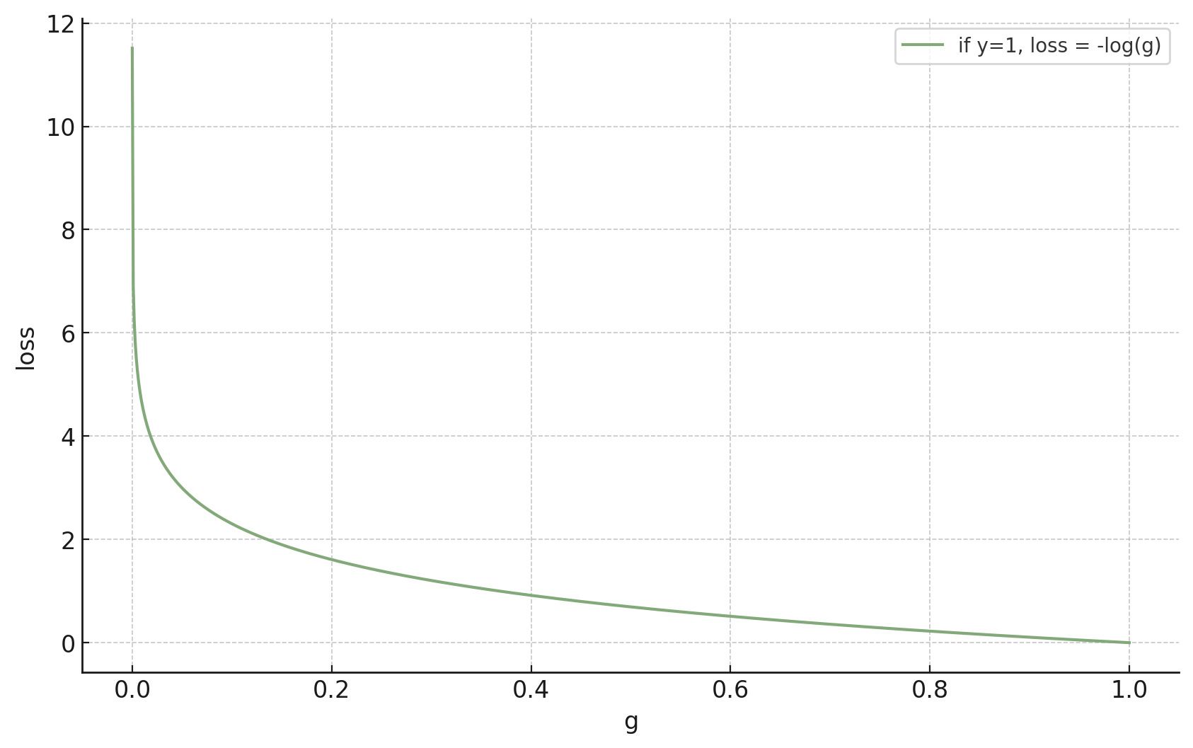
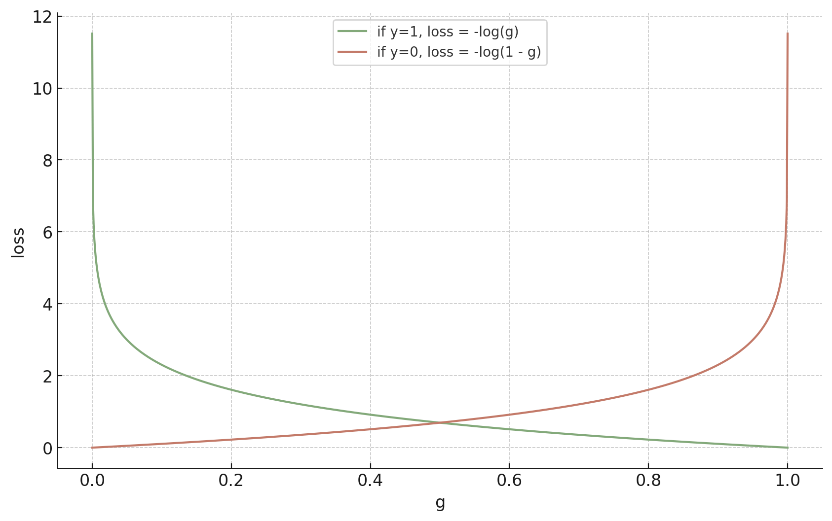
\mathcal{L}_{01}(g, y)=\left\{\begin{array}{ll} 0 & \text { if } g = y \\ 1 & \text { otherwise } \end{array}\right .

\mathcal{L}_{\text{nll}}(g, y)

if true label \(y=1,\) we'd like guess \(g\) to just be \(1\)... difficult ask

now:

if true label \(y=1,\) we'd like the guess \(g\) to gradually approach \(1\)

👇

previously:

:=-\log(g)

= \mathcal{L}_{\text{nll}}(g, 1)

negative

log

likelihood

\(g=\sigma\left(\cdot\right):\) the model's confidence or estimated likelihood that feature \(x\) belongs to the positive class.

training data:

true label \(y\) is \(1\)

👇

\mathcal{L}_{\text{nll}}(g, y)

:=-\log(g)

= \mathcal{L}_{\text{nll}}(g, 1)

\mathcal{L}_{\text{nll}}(g, y)

if true label \(y=0,\) we'd like the guess \(g\) to gradually approach \(0\)

👇

:=-\log(1-g)

= \mathcal{L}_{\text{nll}}(g, 0)

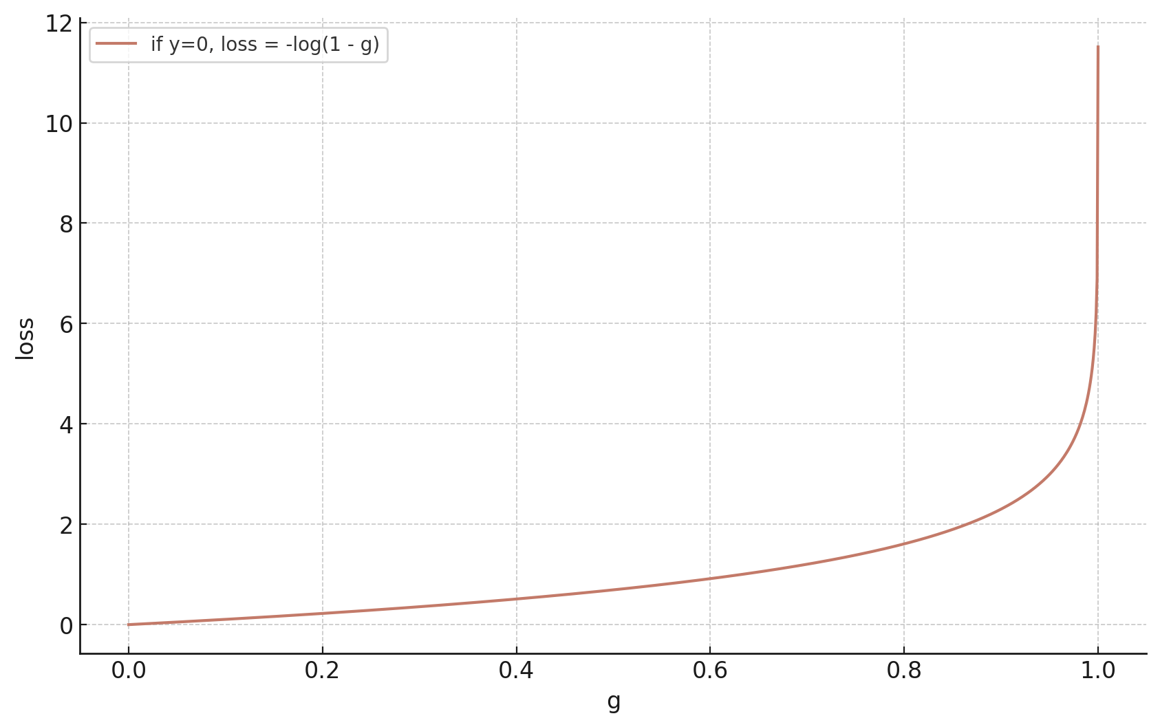
\(g = \sigma\left(\cdot\right):\) the model's confidence or estimated likelihood that feature \(x\) belongs to the positive class.

\(1-g = 1-\sigma\left(\cdot\right):\) the model's confidence or estimated likelihood that feature \(x\) belongs to the negative class.

training data:

\mathcal{L}_{\text{nll}}(g, y)= \mathcal{L}_{\text{nll}}(g, 0)=-\log(1-g)

true label \(y\) is \(0\)

👇

Combining both cases, since the actual label \(y \in \{+1,0\}\)

= - \left[y \log g +\left(1-y \right) \log \left(1-g\right)\right]

\mathcal{L}_{\text {nll }}(g,y)

training data:

😍

🥺

= - \left[y \log g +\left(1-y \right) \log \left(1-g \right)\right]

\mathcal{L}_{\text {nll }}({ g, y })

When \(y = 1\)

😍

🥺

g(x)=\sigma\left(\theta x+\theta_0\right)

g

= - \log g

training data:

😍

🥺

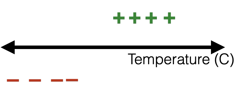
When \(y = 0\)

😍

🥺

g(x)=\sigma\left(\theta x+\theta_0\right)

g

= - \left[y \log g +\left(1-y \right) \log \left(1-g \right)\right]

= - \left[\log \left(1-g \right)\right]

\mathcal{L}_{\text {nll }}({ g, y })

training data:

true label \(y\) is \(1\)

👇

\mathcal{L}_{\text{nll}}(g, y)

:=-\log(g)

= \mathcal{L}_{\text{nll}}(g, 1)

linear

binary classifier

features

parameters

linear combo

predict

\(x \in \mathbb{R}^d\)

\(\theta \in \mathbb{R}^d, \theta_0 \in \mathbb{R}\)

\(\theta^T x +\theta_0\)

\(=z\)

linear logistic

binary classifier

loss

\((g - y)^2 \)

- \left[y \log g +\left(1-y \right) \log \left(1-g\right)\right]

\left\{\begin{array}{ll} 0 & \text { if } g = y \\ 1 & \text { otherwise } \end{array}\right .

\left\{\begin{array}{ll} 1 & \text { if } z>0 \\ 0 & \text { otherwise } \end{array}\right .

\left\{\begin{array}{ll} 1 & \text { if } g = \sigma(z)>0.5 \\ 0 & \text { otherwise } \end{array}\right .

g = z

linear regressor

closed-form or

gradient descent

NP-hard to learn

gradient descent
regularization still important

optimize via

label

\(y \in \mathbb{R}\)

\(y \in \{0,1\}\)

Outline

Linear (binary) classifiers
- to use: separator, normal vector
- to learn: difficult! won't do
Linear logistic (binary) classifiers
- to use: sigmoid
- to learn: negative log-likelihood loss
Multi-class classifiers
- to use: softmax
- to learn: one-hot encoding, cross-entropy loss

Video edited from: HBO, Sillicon Valley

features

parameters

linear combo

predict

\(x \in \mathbb{R}^d\)

\(\theta \in \mathbb{R}^d, \theta_0 \in \mathbb{R}\)

\(\theta^T x +\theta_0\)

\(=z\)

linear logistic binary classifier

if \(\sigma(z) > 0.5\)

otherwise

\left\{ \begin{array}{l} \\ \\ \end{array} \right.

\(1\)

0

🌭

\(x\)

\(z \in \mathbb{R}\)

scalar logit

\sigma(z) \in \mathbb{R}

\(\sigma\left(\cdot\right):\) the model's confidence or estimated likelihood that feature \(x\) belongs to the hotdog class;
\(1-\sigma\left(\cdot\right):\) the not-hotdog class.

scalar likelihood

(raw hotdog-ness)

(normalized probability of hotdog-ness)

to predict among \(K\) categories

say \(K=3\) categories: \(\{\)hot-dog, pizza, salad\(\}\)

\(K\) logits

\text{softmax}(z)\in \mathbb{R}^3

\(K\)-class likelihood

raw likelihood of each category

distribution over the categories

\(z \in \mathbb{R}^3\)

to predict hotdog or not,

a scalar logit suffices

🌭

\(x\)

🌭

\(x\)

\(z \in \mathbb{R}\)

\sigma(z) \in \mathbb{R}

\(K\) classes

two classes

\(\theta \in \mathbb{R}^d, \theta_0 \in \mathbb{R}\)

\(\theta \in \mathbb{R}^{d \times K},\)

\(\theta_0 \in \mathbb{R}^{K}\)

\text{softmax}(z)\in \mathbb{R}^K

\(z \in \mathbb{R}^K\)

🌭

\(x\)

🌭

\(x\)

\(z \in \mathbb{R}\)

\sigma(z) \in \mathbb{R}

raw likelihood of each category

\(K\) classes

two classes

🌭

\(x\)

🌭

\(x\)

\(z \in \mathbb{R}\)

\(z \in \mathbb{R}^K\)

\sigma(z) \in \mathbb{R}

\text{softmax}(z)\in \mathbb{R}^K

raw likelihood of each category

distribution over \(K\) categories

\dots

\left\} \begin{array}{l} \\ \\ \\ \end{array} \right.

\begin{bmatrix} 1 \\ 2 \\ 3 \end{bmatrix}

=\begin{bmatrix} \frac{e^{1}}{e^{1} + e^{2} + e^{3}} \\[6pt] \frac{e^{2}}{e^{1} + e^{2} + e^{3}} \\[6pt] \frac{e^{3}}{e^{1} + e^{2} + e^{3}} \end{bmatrix}

=\begin{bmatrix} 0.0900 \\[6pt] 0.2447 \\[6pt] 0.6653 \end{bmatrix}

\operatorname{softmax}

\left( \begin{array}{l} \\ \\ \\ \end{array} \right.

\left) \begin{array}{l} \\ \\ \\ \end{array} \right.

each output entry is between 0 and 1, and their sum is 1

max in the input

"soft" max'd in the output

\operatorname{softmax}(z) := \begin{bmatrix} \frac{\exp(z_1)}{\sum_{k=1}^K \exp(z_k)} \\[6pt] \vdots \\[6pt] \frac{\exp(z_K)}{\sum_{k=1}^K \exp(z_k)} \end{bmatrix}

softmax:

\mathbb{R}^K \to \mathbb{R}^K

e.g.

sigmoid

= \frac{\exp(z)}{\exp(z) +\exp (0)}

\sigma(z):=\frac{1}{1+\exp (-z)}

\mathbb{R} \to \mathbb{R}

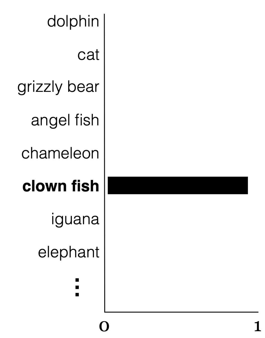
predict the category with the highest softmax score

\operatorname{softmax}(z) := \begin{bmatrix} \frac{\exp(z_1)}{\sum_{k=1}^K \exp(z_k)} \\[6pt] \vdots \\[6pt] \frac{\exp(z_K)}{\sum_{k=1}^K \exp(z_k)} \end{bmatrix}

softmax:

\mathbb{R}^K \to \mathbb{R}^K

predict positive if \(\sigma(z)>0.5 = \sigma(0)\)

equivalently, predicting the category with the largest raw logit.

implicit logit for the negative class

features

parameters

linear combo

predict

\(x \in \mathbb{R}^d\)

\(\theta \in \mathbb{R}^d, \theta_0 \in \mathbb{R}\)

\(\theta^T x +\theta_0\)

\(=z \in \mathbb{R}\)

linear logistic

binary classifier

one-out-of-\(K\) classifier

\(\theta \in \mathbb{R}^{d \times K},\)

\(=z \in \mathbb{R}^{K}\)

\(\theta^T x +\theta_0\)

predict positive if \(\sigma(z)>\sigma(0)\)

predict the category with the highest softmax score

\operatorname{softmax}(z) = \begin{bmatrix} \frac{\exp(z_1)}{\sum_{k=1}^K \exp(z_k)} \\[6pt] \vdots \\[6pt] \frac{\exp(z_K)}{\sum_{k=1}^K \exp(z_k)} \end{bmatrix}

\sigma(z) = \frac{\exp(z)}{\exp(0) +\exp (z)}

\(\theta_0 \in \mathbb{R}^{K}\)

Outline

Linear (binary) classifiers
- to use: separator, normal vector
- to learn: difficult! won't do
Linear logistic (binary) classifiers
- to use: sigmoid
- to learn: negative log-likelihood loss
Multi-class classifiers
- to use: softmax
- to learn: one-hot encoding, cross-entropy loss

image adapted from Phillip Isola

K =3

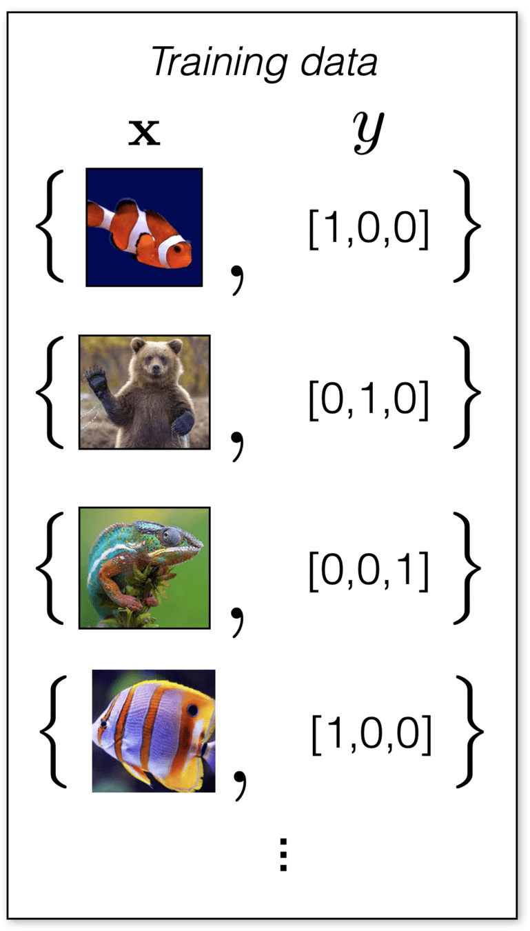
One-hot encoding:

Generalizes from {0,1} binary labels
Encode the \(K\) classes as an \(\mathbb{R}^K\) vector, with a single 1 (hot) and 0s elsewhere.

column vectors

flipped due to slides real-estate

\mathcal{L}_{\mathrm{nllm}}({g}, y)=-\sum_{{k}=1}^{{K}}y_{{k}} \cdot \log \left({g}_{{k}}\right)

Generalizes negative log likelihood loss \(\mathcal{L}_{\mathrm{nll}}({g}, {y})= - \left[y \log g +\left(1-y \right) \log \left(1-g \right)\right]\)
Although this is written as a sum over \(K\) terms, for a given training data point, only the term corresponding to its true class label contributes, since all other \(y_k=0\)

Negative log-likelihood \(K-\) classes loss (aka, cross-entropy)

\(y:\)one-hot encoding label

\(y_{{k}}:\) \(k\)th entry in \(y\), either 0 or 1

\(g:\) softmax output

\(g_{{k}}:\) probability or confidence of belonging in class \(k\)

current prediction

\(g=\text{softmax}(\cdot)\)

feature \(x\)

true label \(y\)

\log(g)

y

[0,0,0,0,0,1,0,0, \ldots]

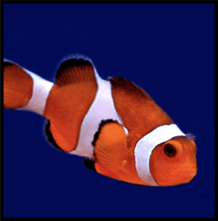
image adapted from Phillip Isola

loss \(\mathcal{L}_{\mathrm{nllm}}({g}, y)\\=-\sum_{{k}=1}^{{K}}y_{{k}} \cdot \log \left({g}_{\mathrm{k}}\right)\)

feature \(x\)

true label \(y\)

\log(g)

y

[0,0,1,0,0,0,0,0, \ldots]

current prediction

\(g=\text{softmax}(\cdot)\)

image adapted from Phillip Isola

loss \(\mathcal{L}_{\mathrm{nllm}}({g}, y)\\=-\sum_{{k}=1}^{{K}}y_{{k}} \cdot \log \left({g}_{\mathrm{k}}\right)\)

Classification

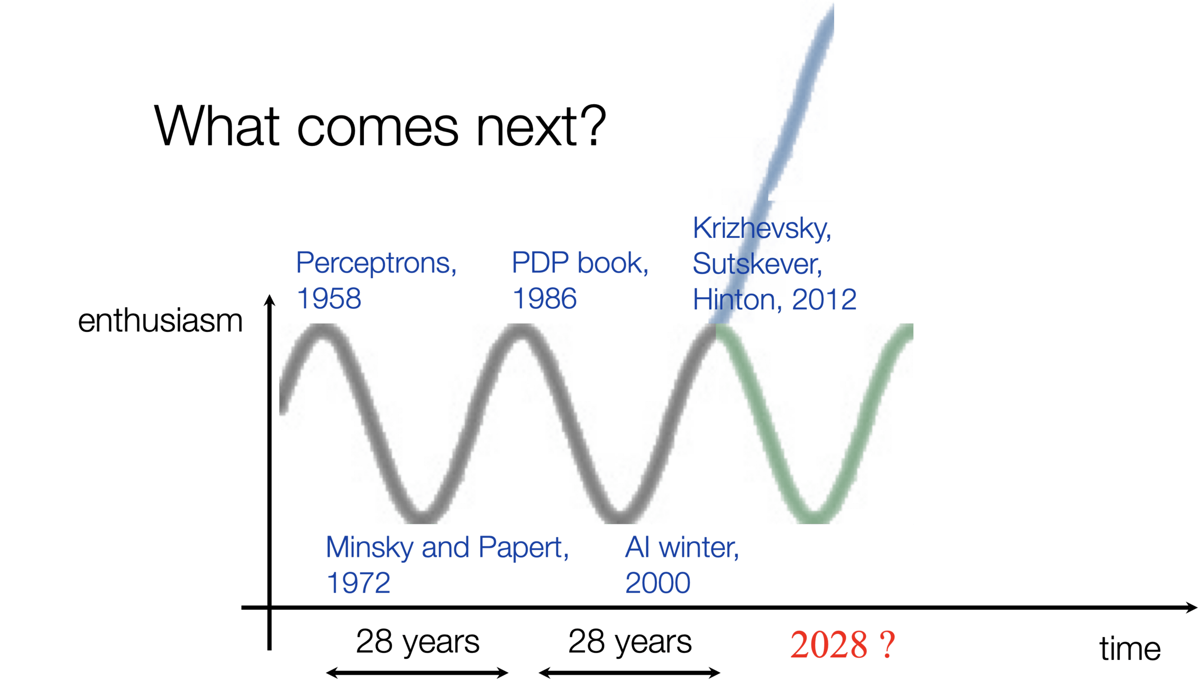
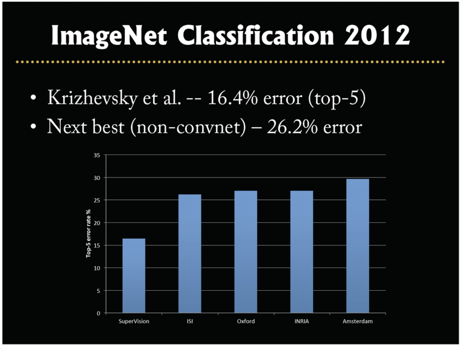
Image classification played a pivotal role in kicking off the current wave of AI enthusiasm.

Summary

Classification: a supervised learning problem, similar to regression, but where the output/label is in a discrete set.
Binary classification: only two possible label values.
Linear binary classification: think of \(\theta\) and \(\theta_0\) as defining a hyperplane that cuts the d-dimensional feature space into two half-spaces.
0-1 loss: a natural loss function for classification, BUT, hard to optimize.
Sigmoid function: smoother and probabilistic step function, motivation and properties.
NLL loss: smooth loss and has nice probabilistic motivations. Can optimize via (S)GD.
Regularization is still important.
The generalization to multi-class via (one-hot encoding, and softmax mechanism)
Other ways to generalize to multi-class (see hw/lab)

Thanks!

We'd love to hear your thoughts.

\rightarrow

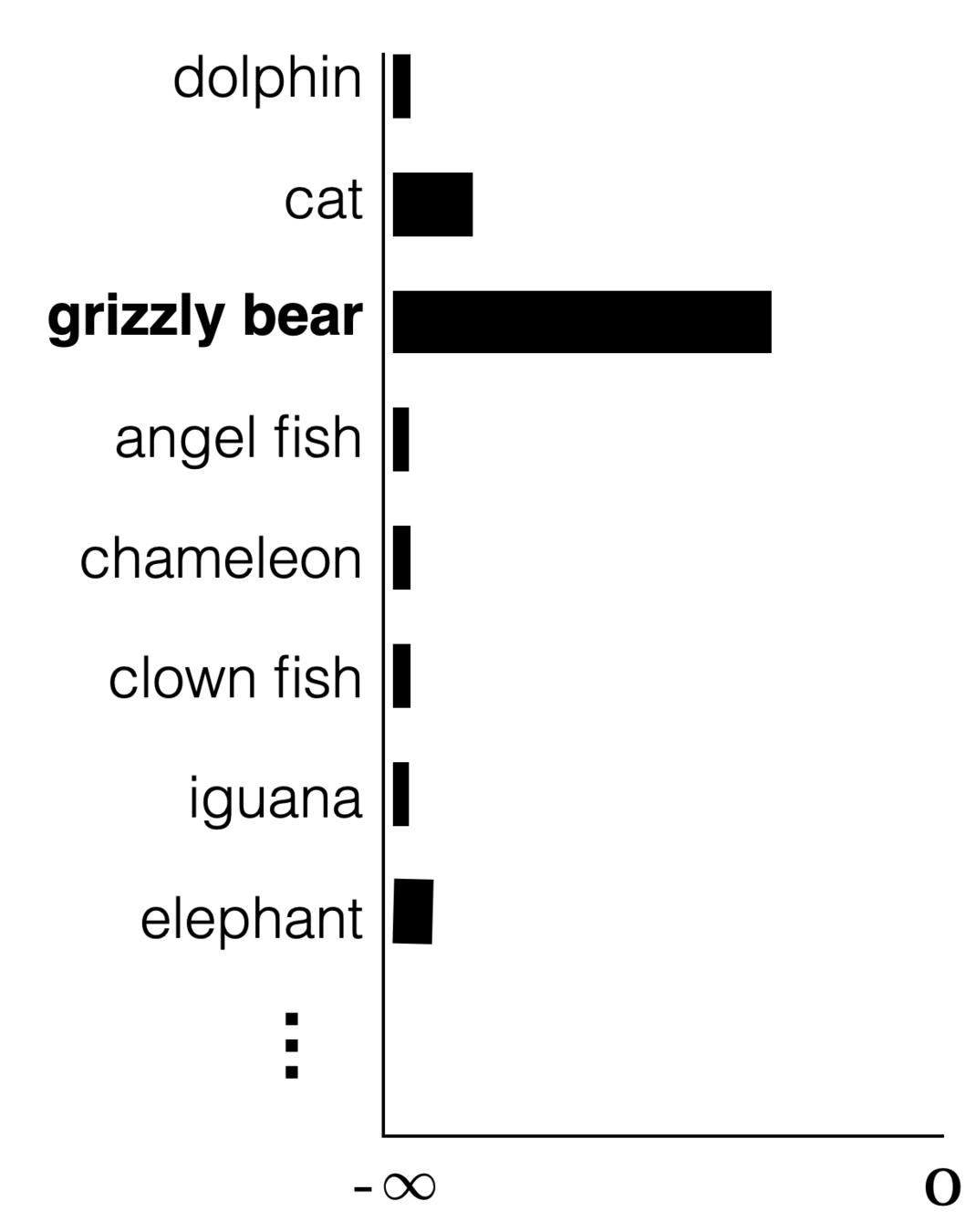
new feature

"Fish"

new prediction

{"Fish", "Grizzly", "Chameleon", ...}

\boxed{h}

\downarrow

x

y \in

\downarrow

Regression

Algorithm

🧠⚙️
hypothesis class
loss function
hyperparameters

images adapted from Phillip Isola

features

label

🌭

\(x\)

\(\theta^T x +\theta_0\)

\(z \in \mathbb{R}\)

if we want to predict among \(K\) categories

say \(K=4\) categories: \(\{\)hot-dog, pizza, pasta, salad\(\}\)

❓

\(z \in \mathbb{R}^4\)

\left\{ \begin{array}{l} \\ \\ \end{array} \right.

distribution over these 4 categories

4 logits, each one a raw summary of the corresponding food category

🌭

\(x\)

\(\theta^T x +\theta_0\)

\(z \in \mathbb{R}^3\)

\left\{ \begin{array}{l} \\ \\ \end{array} \right.

distribution over these 3 categories

❓

if we want to predict among \(K\) categories

say \(K=3\) categories: \(\{\)hot-dog, pizza, salad\(\}\)

Outline

Linear (binary) classifiers
- to use: separator, normal vector
- to learn: difficult! won't do
Linear logistic (binary) classifiers
- to use: sigmoid
- to learn: negative log-likelihood loss
Multi-class classifiers
- to use: softmax
- to learn: one-hot encoding, cross-entropy loss

Linear Logistic Classifier

Mainly motivated to address the gradient issue in learning a "vanilla" linear classifier
- The gradient issue is caused by both the 0/1 loss, and the sign functions nested in.

\mathcal{L}_{01}(x^{(i)}, y^{(i)}; \theta, \theta_0)=\left\{\begin{array}{ll} 0 & \text { if } \operatorname{sign}\left(\theta^{\top} x^{(i)}+\theta_0\right) = y^{(i)} \\ 1 & \text { otherwise } \end{array}\right .

But has nice probabilistic interpretation too.
As before, let's first look at how to make prediction with a given linear logistic classifier

(Binary) Linear Logistic Classifier

Each data point:
- features \([x_1, x_2, \dots x_d]\)
- label \(y \in\){positive, negative}
A (binary) linear logistic classifier is parameterized by \([\theta_1, \theta_2, \dots, \theta_d, \theta_0]\)
To use a given classifier make prediction:
- do linear combination: \(z =({\theta_1}x_1 + \theta_2x_2 + \dots + \theta_dx_d) + \theta_0\)
- predict positive label if

otherwise, negative label.

\sigma(z) = \sigma\left(\theta^{\top} x+\theta_0\right)

= \frac{1}{1+e^{-z}}

= \frac{1}{1+e^{-\left(\theta^{\top} x+\theta_0\right)}}

> 0.5

: a smooth step function

= \frac{1}{1+e^{-z}}

Sigmoid

if \(\sigma(z) > 0.5\)

otherwise

\left\{ \begin{array}{l} \\ \\ \end{array} \right.

\(1\)

0

🌭

\(x\)

\(\theta^T x +\theta_0\)

\(z \in \mathbb{R}\)

\(\sigma(z) :\) model's confidence the input \(x\) is a hot-dog

learned scalar "summary" of "hot-dog-ness"

\(1-\sigma(z) :\) model's confidence the input \(x\) is not a hot-dog

fixed baseline of "non-hot-dog-ness"

training data:

😍

🥺

Recall, the labels \(y \in \{+1,0\}\)

g(x)=\sigma\left(\theta x+\theta_0\right)

= -[\text { actual } \cdot \log (\text { guess })+(1-\text { actual }) \cdot \log (1-\text { guess })]

= - \left[y \log g +\left(1-y \right) \log \left(1-g\right)\right]

\mathcal{L}_{\text {nll }}(\text { guess, actual })

g

training data:

😍

🥺

= - \left[y \log g +\left(1-y \right) \log \left(1-g \right)\right]

\mathcal{L}_{\text {nll }}(\text { guess, actual })

If \(y = 1\)

😍

🥺

g(x)=\sigma\left(\theta x+\theta_0\right)

g

= - \log g

training data:

😍

🥺

If \(y = 0\)

😍

🥺

g(x)=\sigma\left(\theta x+\theta_0\right)

g

= - \left[y \log g +\left(1-y \right) \log \left(1-g \right)\right]

\mathcal{L}_{\text {nll }}(\text { guess, actual })

= - \left[\log \left(1-g \right)\right]

training data:

= - \left[y \log g +\left(1-y \right) \log \left(1-g \right)\right]

\mathcal{L}_{\text {nll }}(\text { guess, actual })

= - \log g

Lecture 4: Linear Classification

Intro to Machine Learning

Outline

Outline

Outline

Outline

Outline

Outline

Outline

Classification

Summary

Thanks!

Outline

Linear Logistic Classifier

(Binary) Linear Logistic Classifier