

Lecture 8: Representation Learning
Intro to Machine Learning

Outline
- Neural networks are representation learners
- Auto-encoders
- Word embeddings
- (Some recent representation learning ideas)
- Neural networks are representation learners
- Auto-encoders
- Word embeddings
- (Some recent representation learning ideas)
layer
linear combo
activations
Recap:
layer
input
neuron
learnable weights
hidden
output
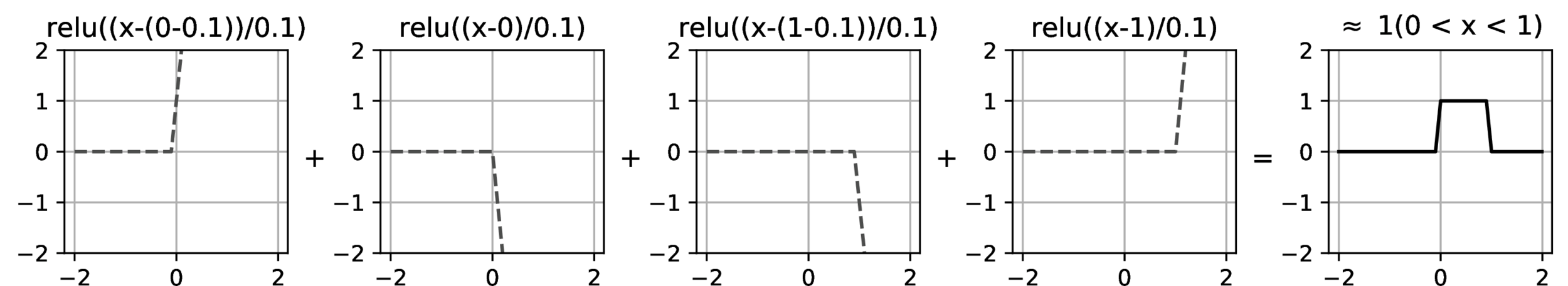
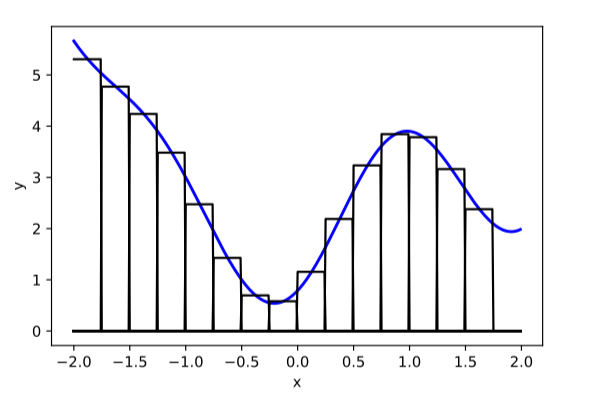
asymptotically, can approximate any function!
[images credit: visionbook.mit.edu]
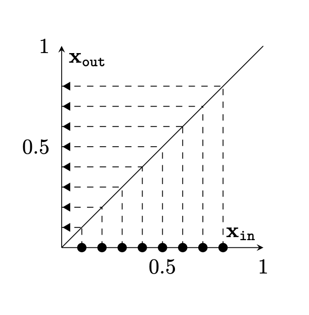
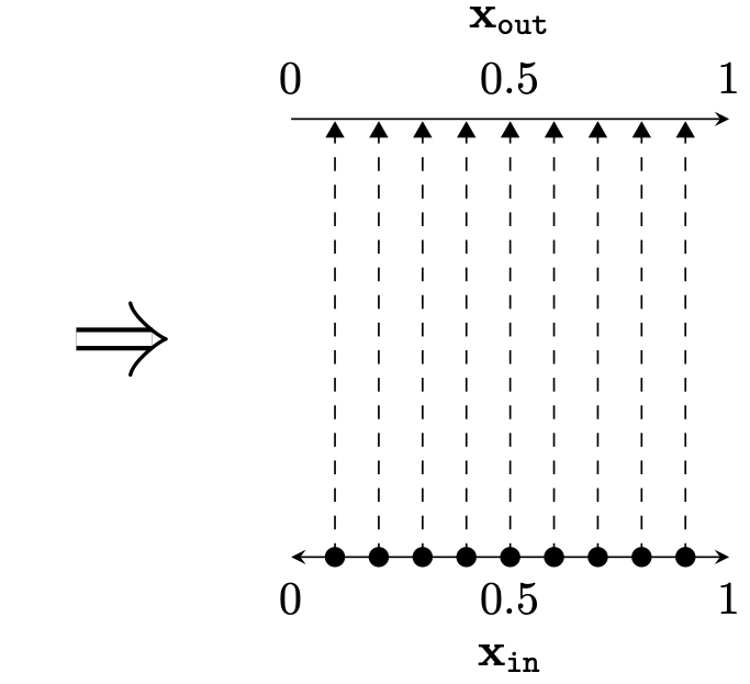
Two different ways to visualize a function
[images credit: visionbook.mit.edu]
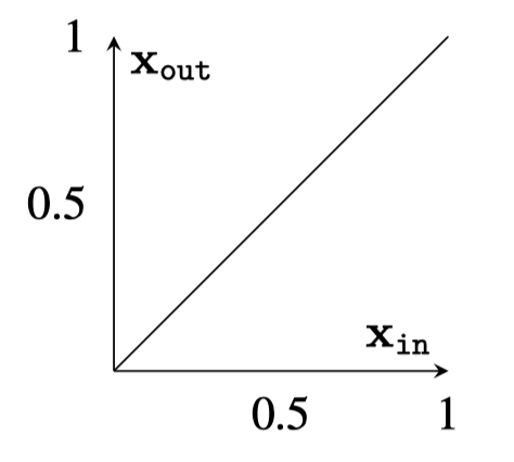
e.g. the identity function
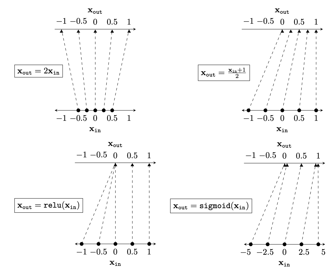
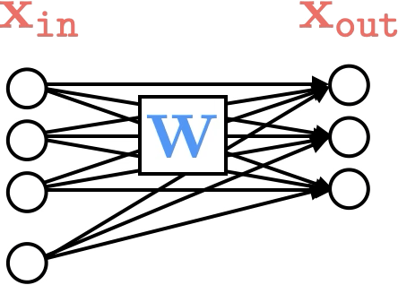
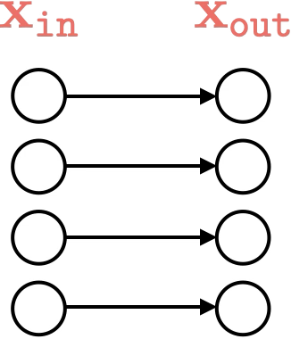
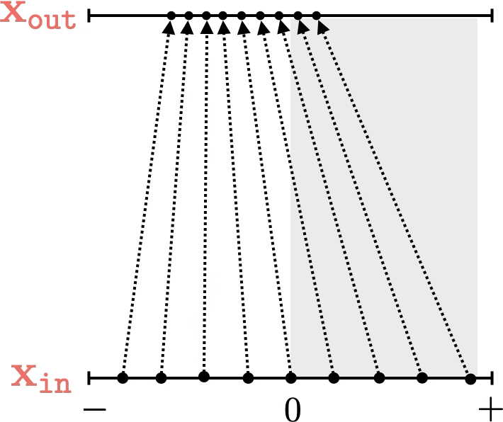
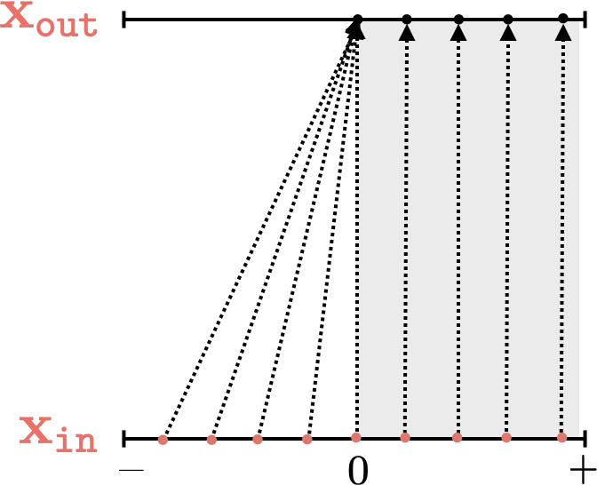
Representation transformations for a variety of neural net operations
[images credit: visionbook.mit.edu]
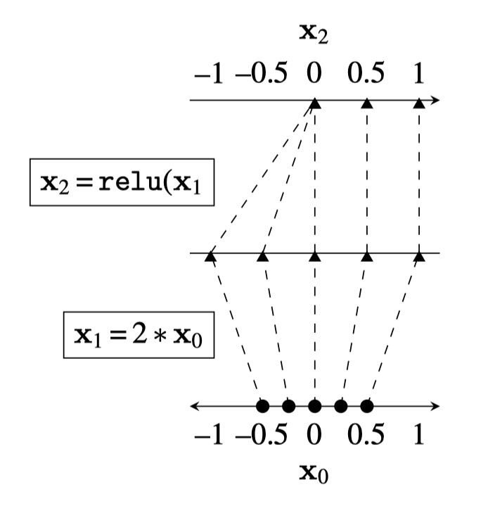
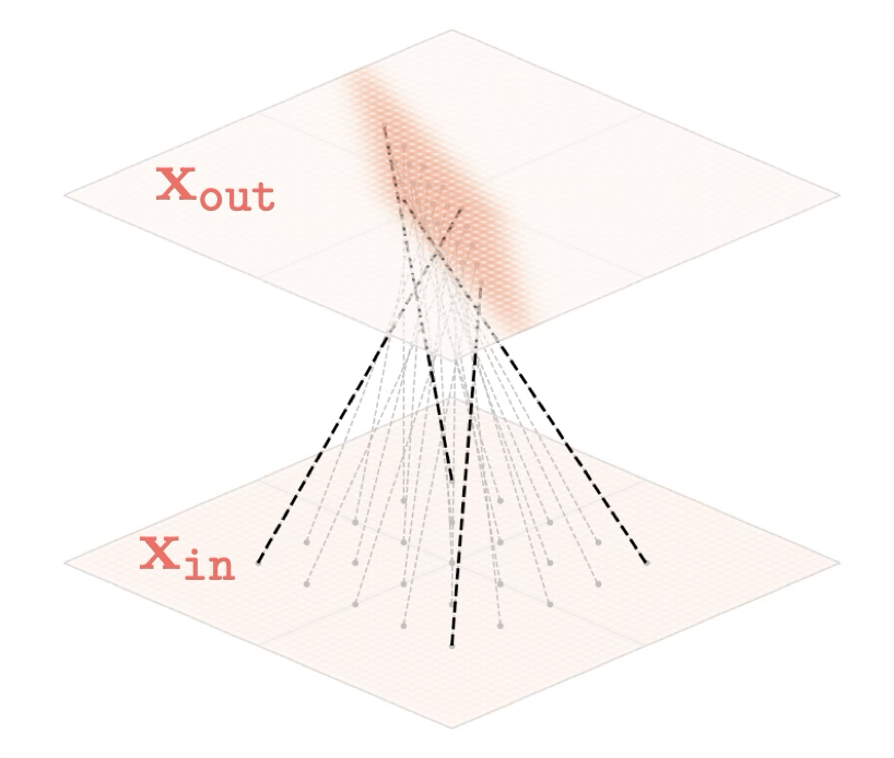
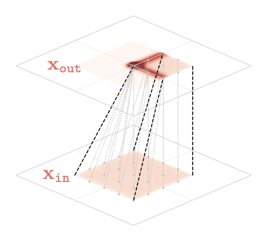
and stack of neural net operations
[images credit: visionbook.mit.edu]
wiring graph
equation
mapping 1D
mapping 2D


[images credit: visionbook.mit.edu]
[images credit: visionbook.mit.edu]
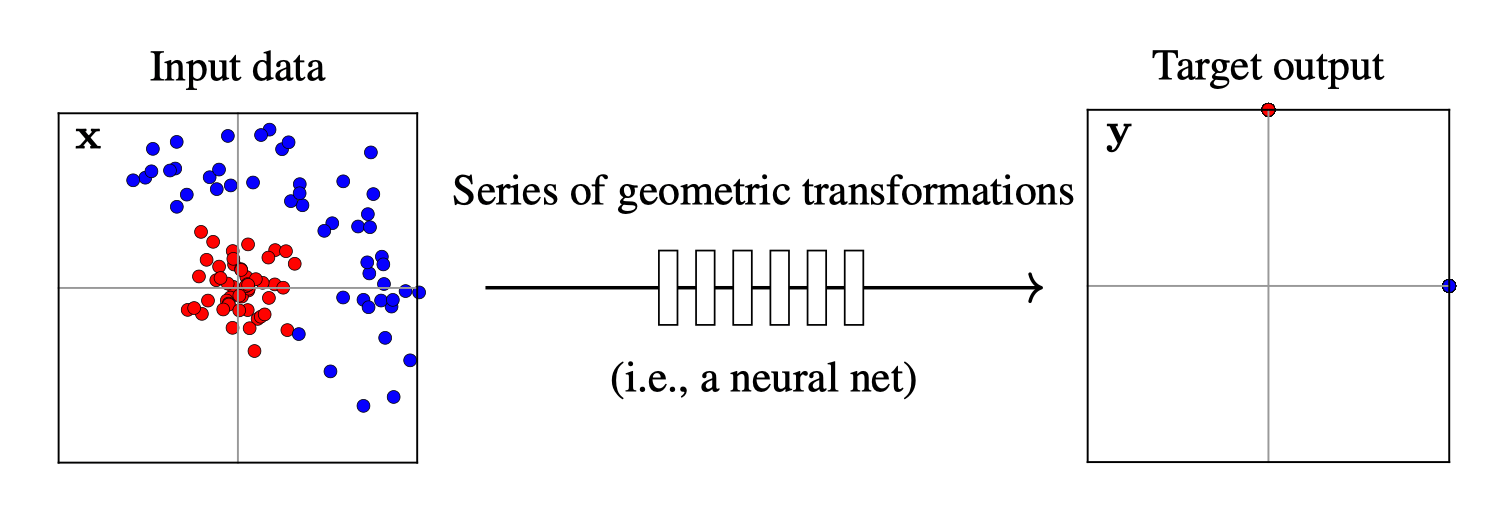
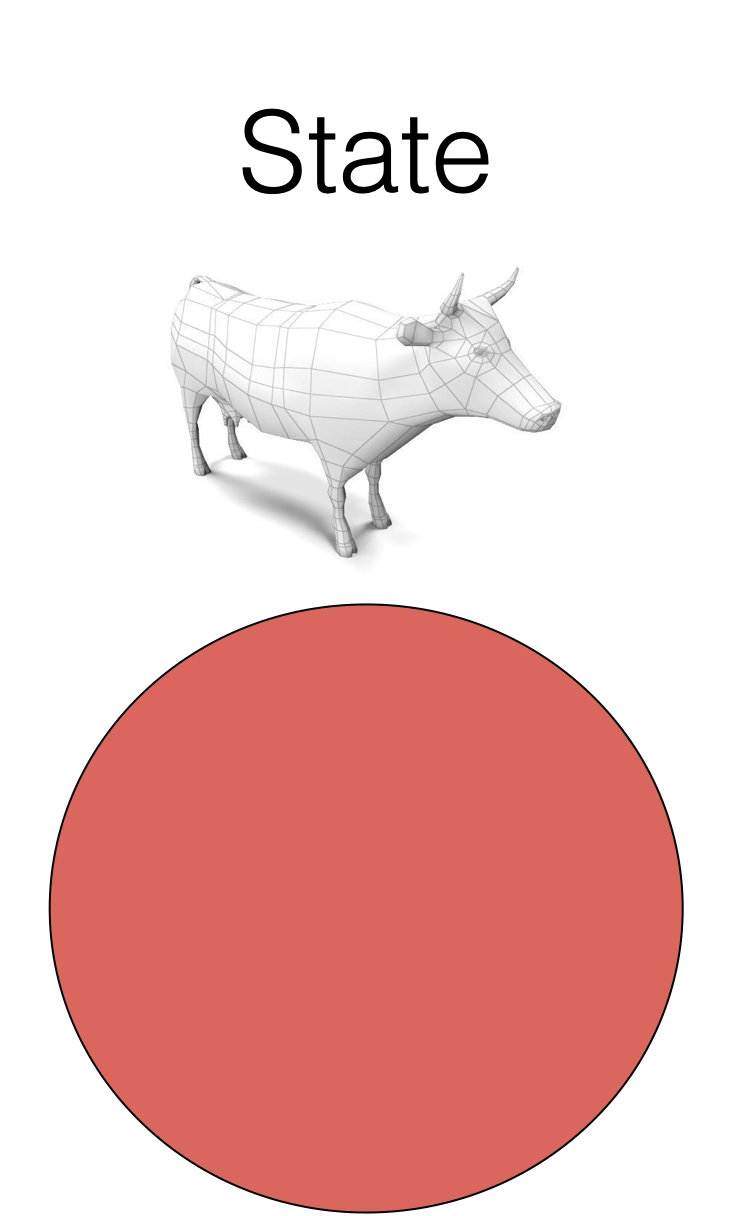
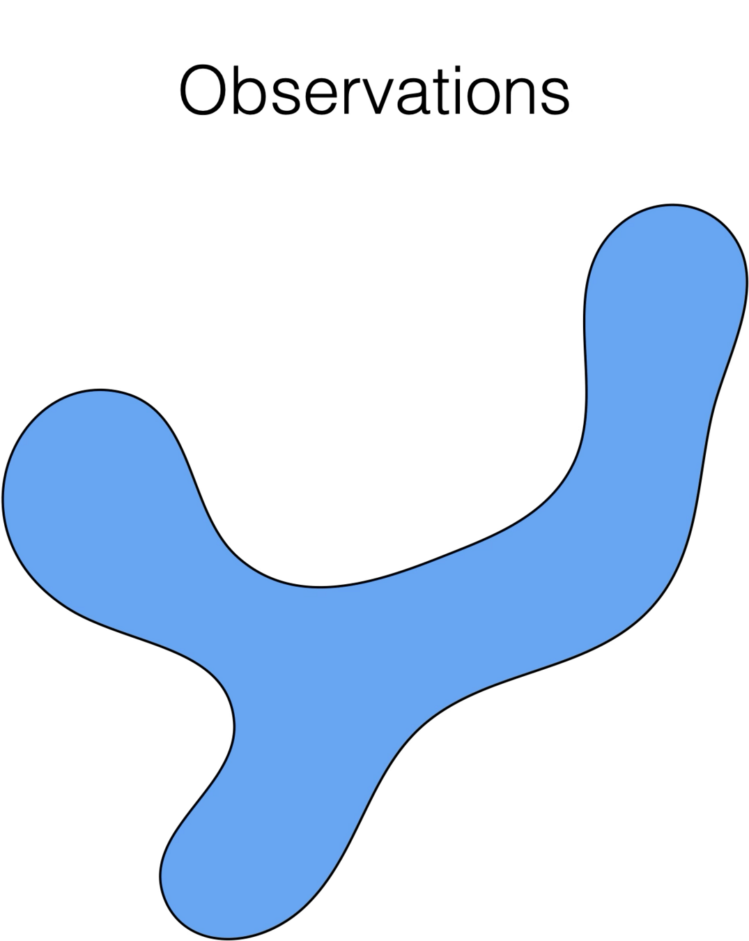
What does training a neural net classifier look like?
Training data
maps from complex data space to desired target space
[images credit: visionbook.mit.edu]

[images credit: visionbook.mit.edu]
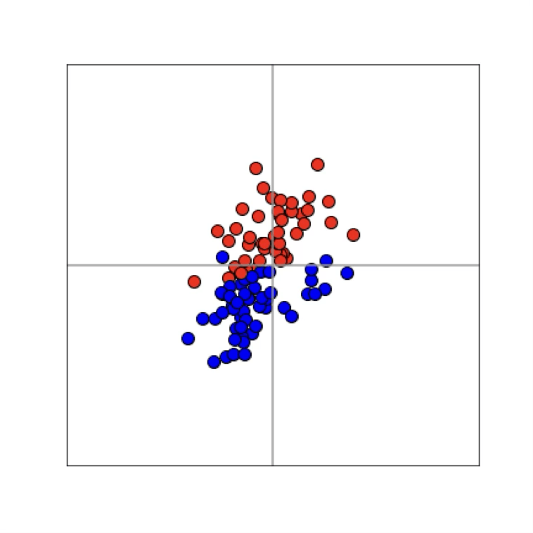
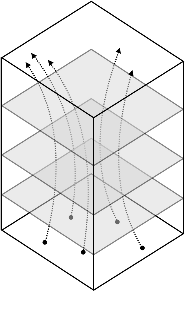
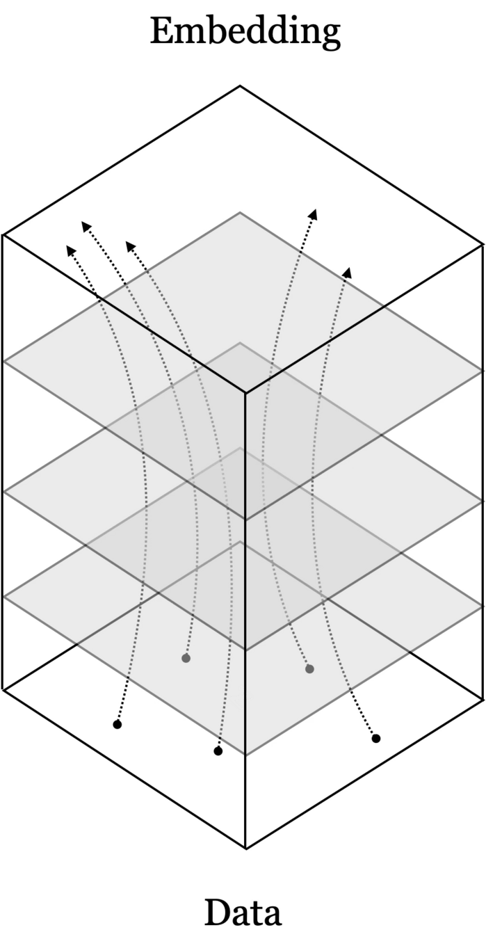
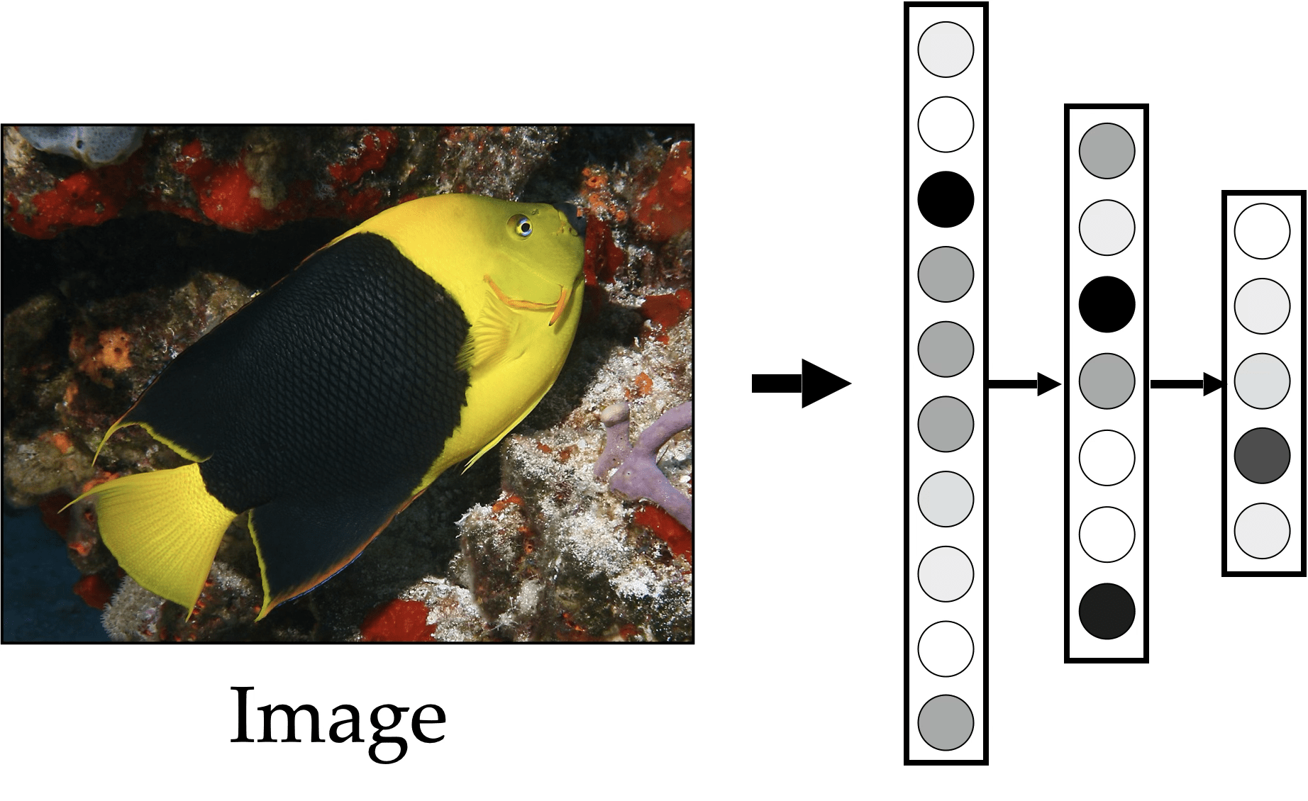
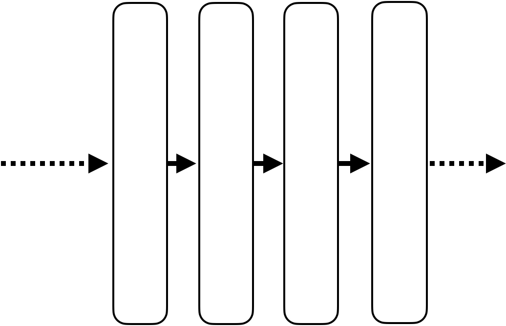
Deep neural nets transform datapoints, layer by layer
Each layer is a different representation, aka embedding, of the data
[images credit: visionbook.mit.edu]
From data to latent embeddings: representation learning
(From latent embeddings to data: generative modeling)
Representation learning
Generative modeling
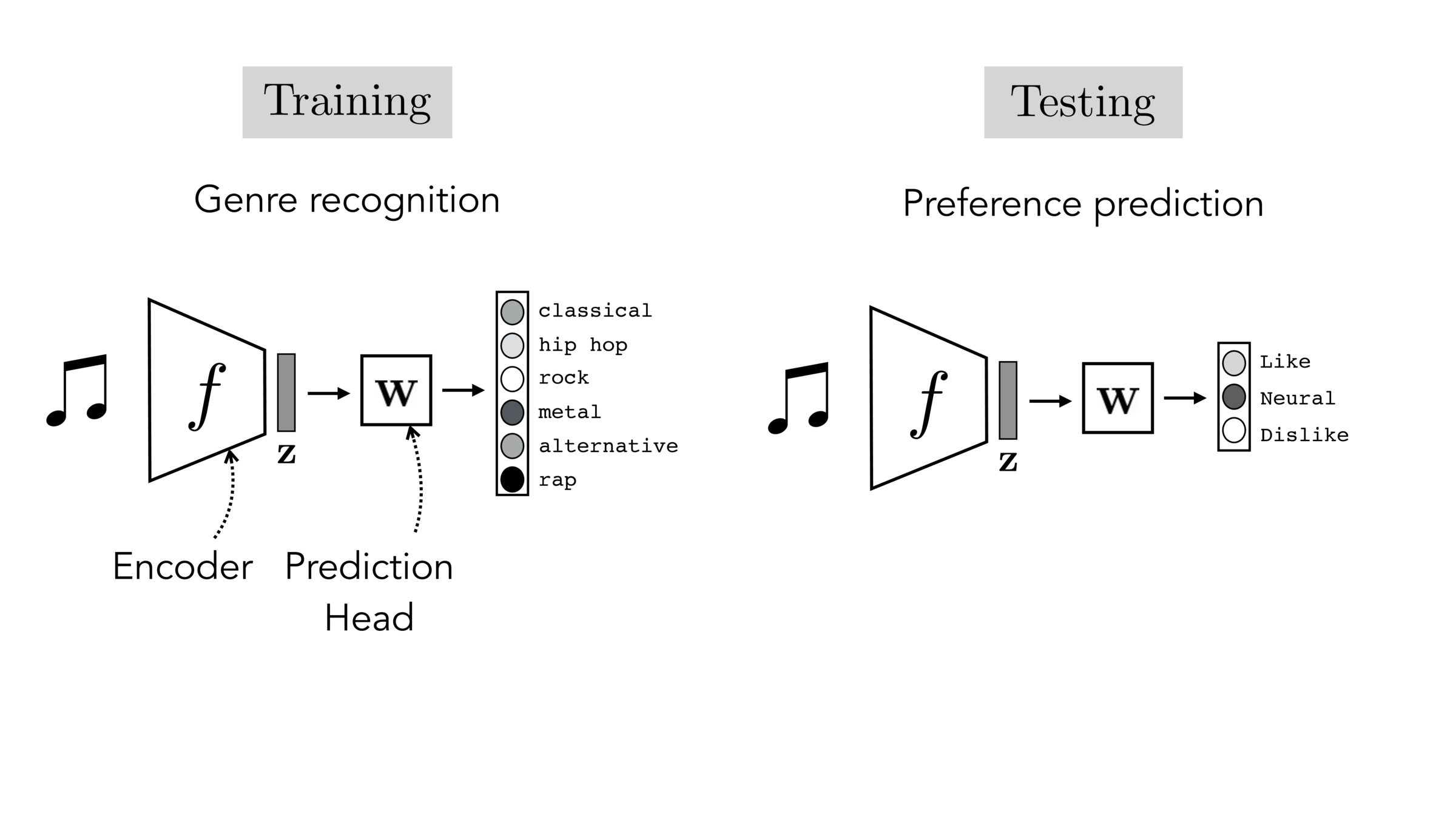
Often, what we will be “tested” on is not what we were trained on.
[images credit: visionbook.mit.edu]
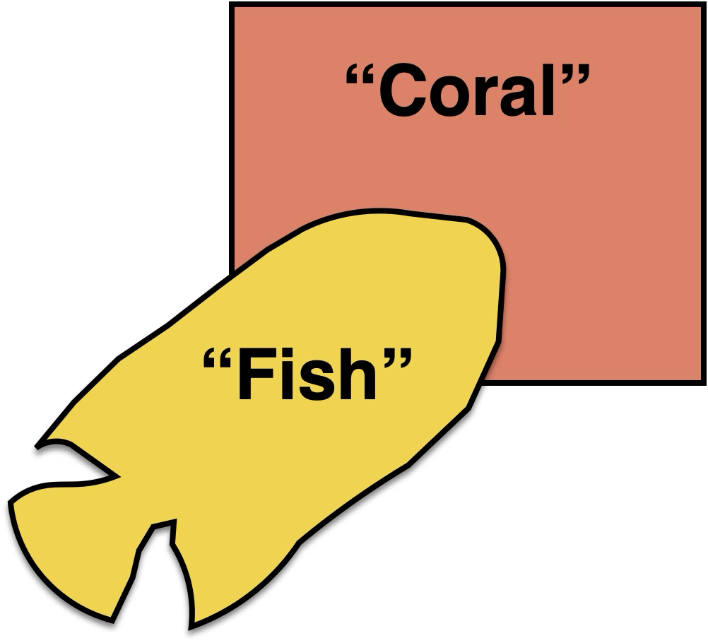
"common"-sense representation
task-specific prediction
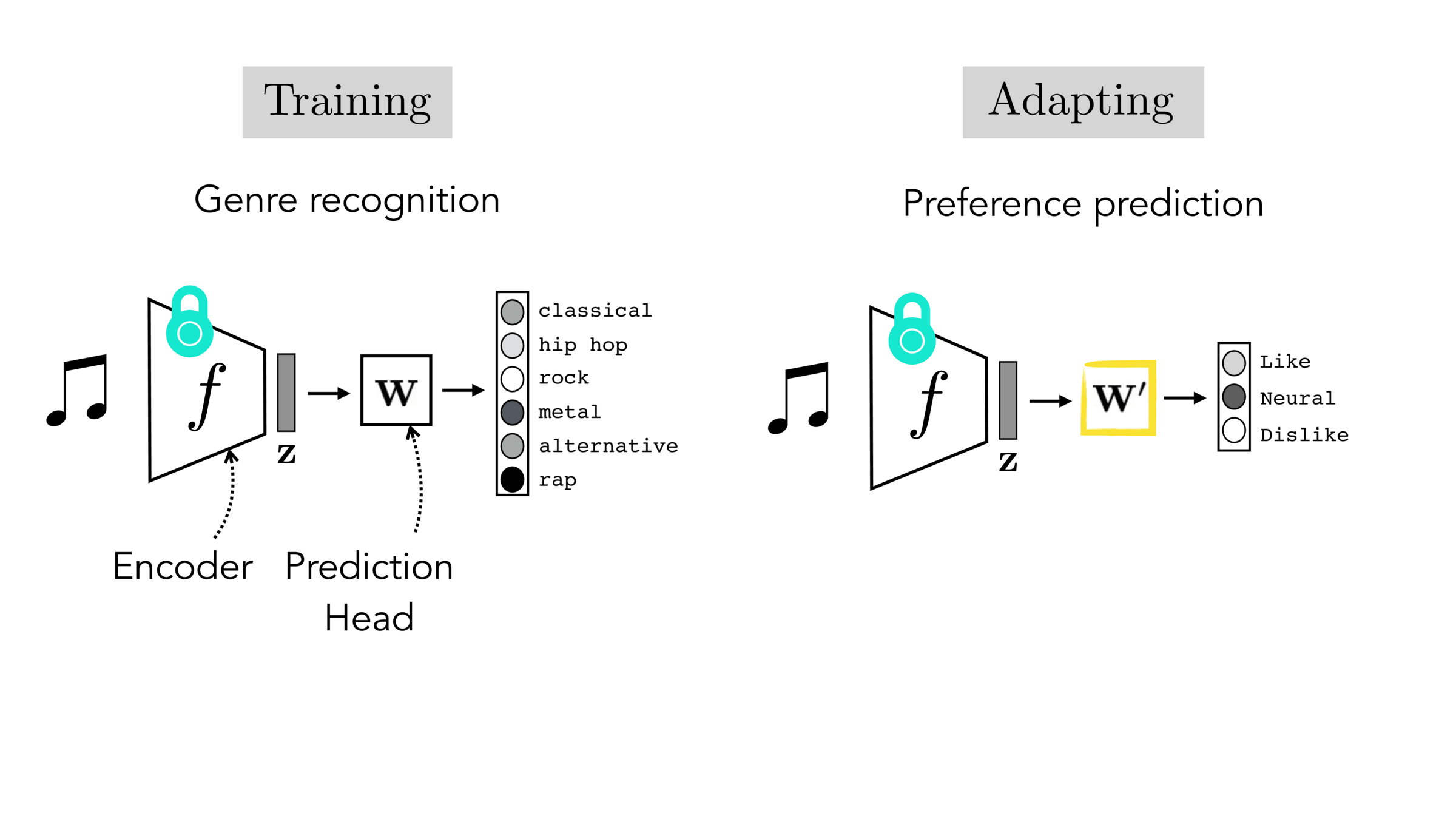
Final-layer adaptation: freeze \(f\), train a new final layer to new target data
[images credit: visionbook.mit.edu]
"common"-sense representation
task-specific prediction
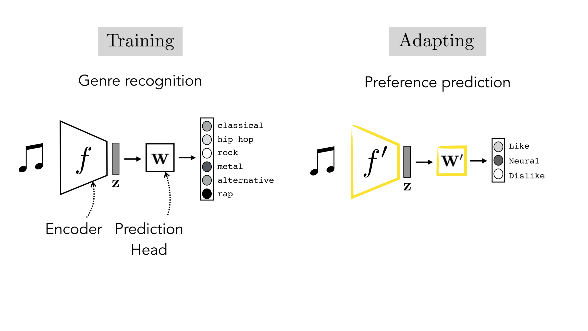
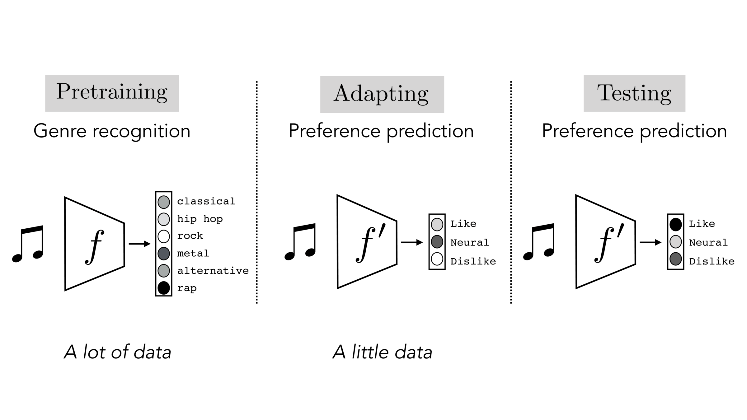
Finetuning: initialize \(f’\) as \(f\), then continue training for \(f'\) as well, on new target data
[images credit: visionbook.mit.edu]
"common"-sense representation
task-specific prediction
[images credit: visionbook.mit.edu]
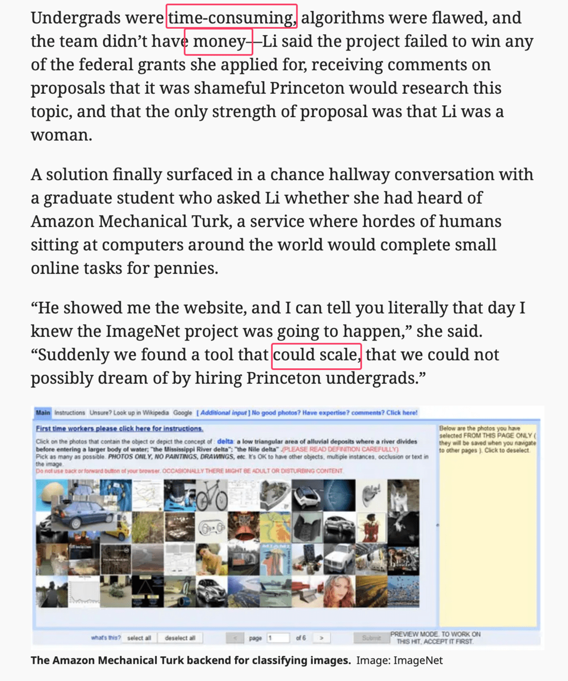
ImageNet also taught us that labeling 14 million images by hand is brutal.
Label prediction (supervised learning)
Label
$$x$$
$$y$$
Features
Labels \(y\) are expensive…
Unlabeled features \(x\) are abundant
Can we learn useful things with just \(x\)?
Outline
- Neural networks are representation learners
- Auto-encoders
- Word embeddings
- (Some recent representation learning ideas)
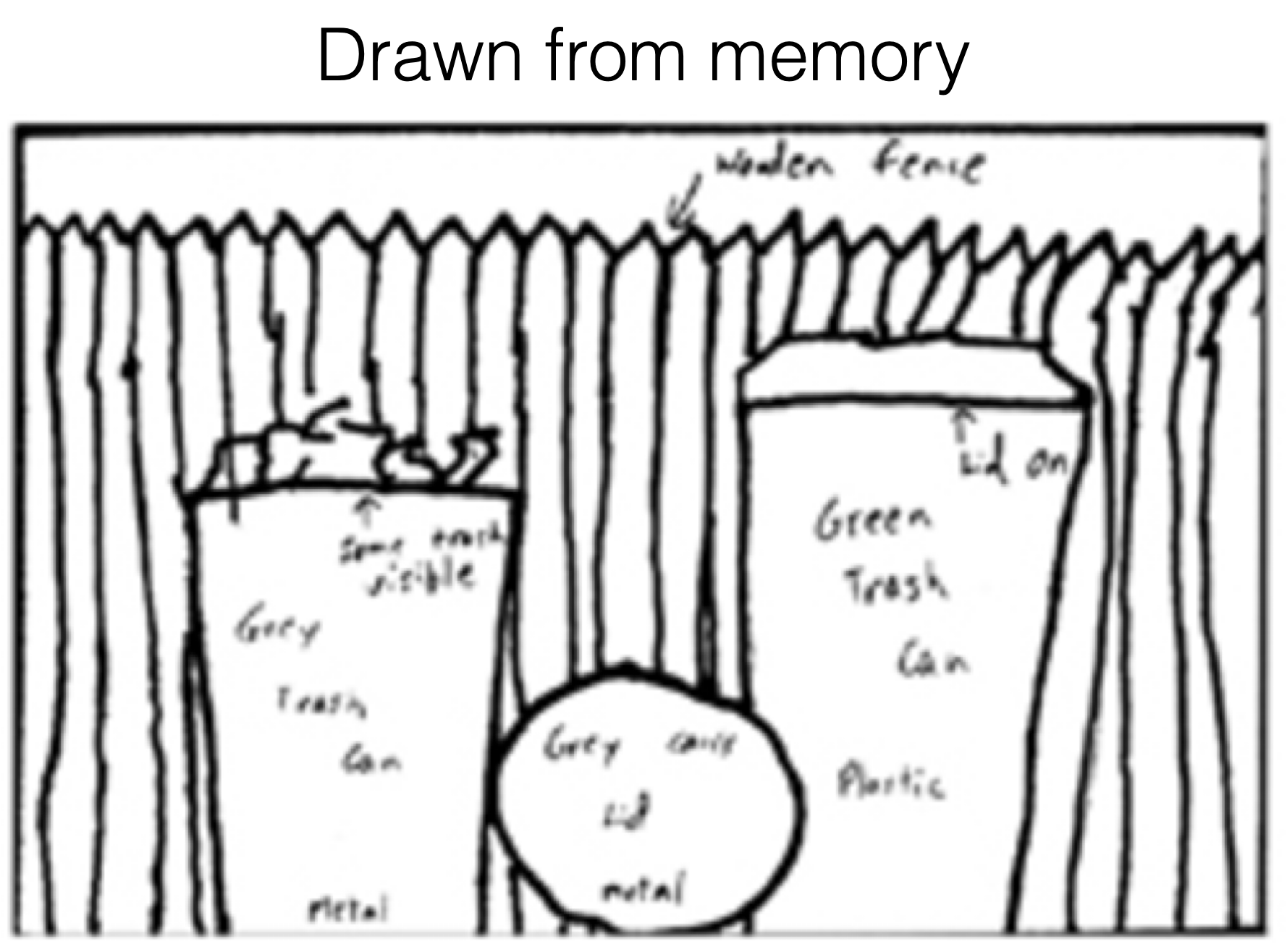
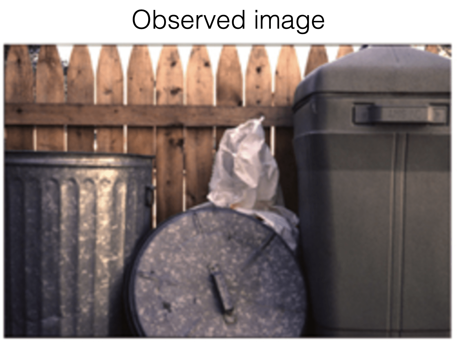
[Bartlett, 1932]
[Intraub & Richardson, 1989]
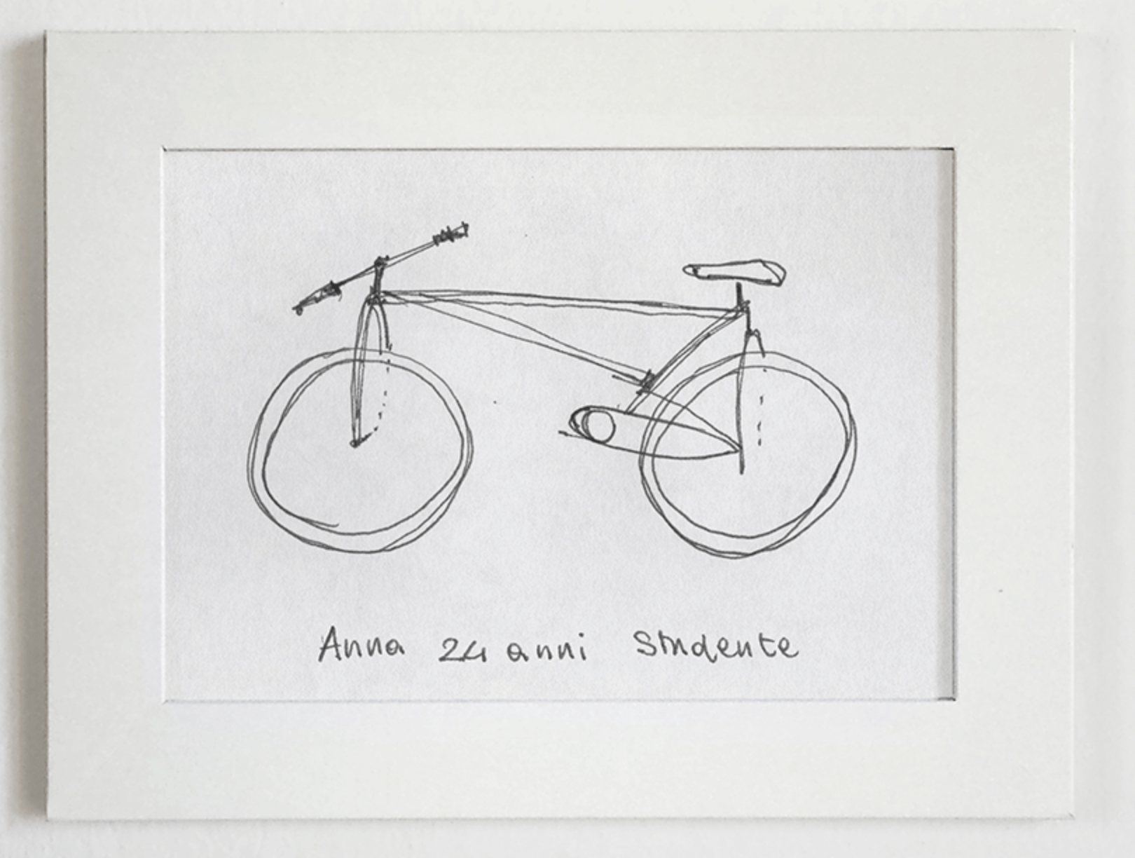
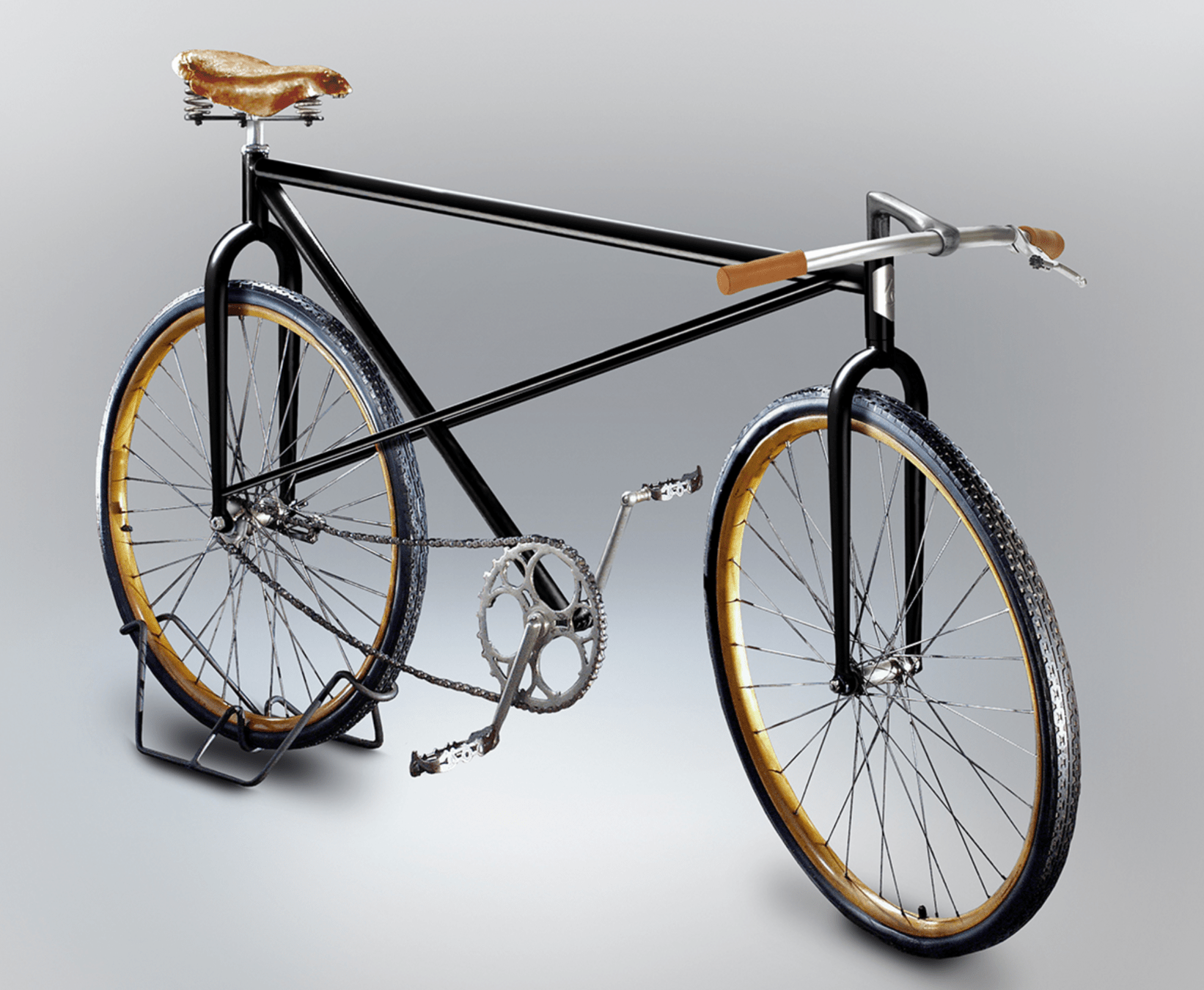
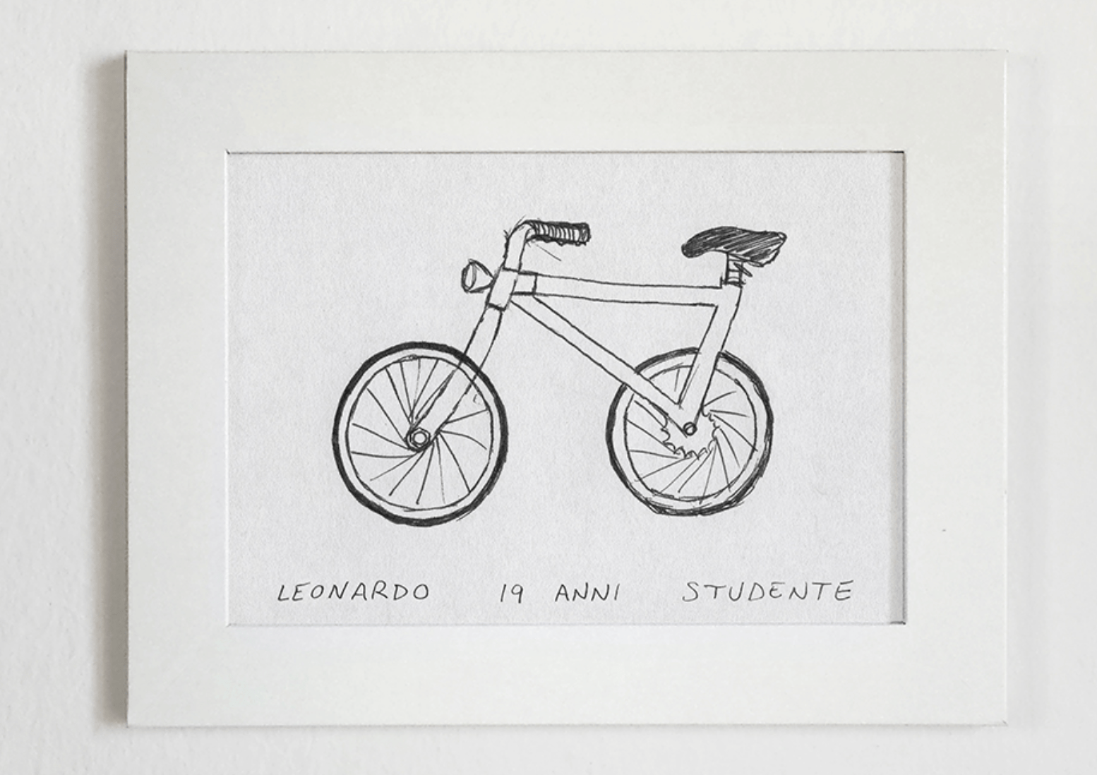
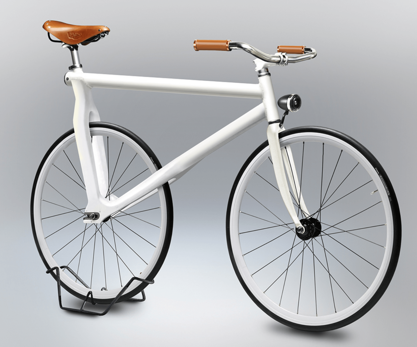
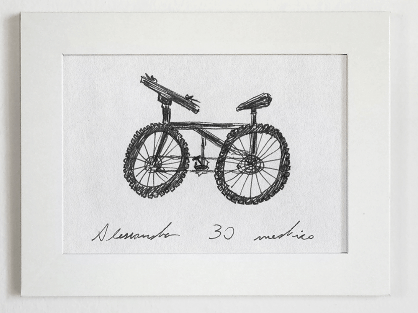
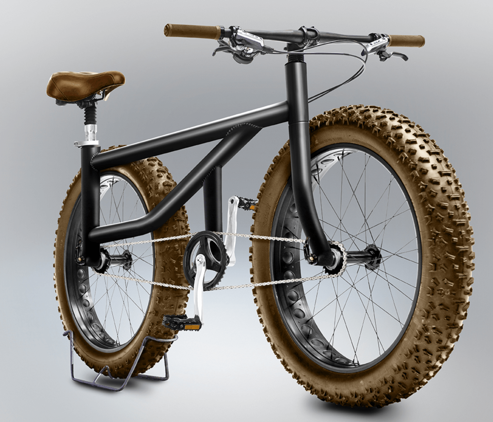
[https://www.behance.net/gallery/35437979/Velocipedia]
🧠
humans also learn representations
[images credit: visionbook.mit.edu]
- Compact (minimal)
- Explanatory (roughly sufficient)
- Disentangled (independent factors)
- Interpretable (understandable by humans)
- Make subsequent problem solving easy
[See “Representation Learning”, Bengio 2013, for more commentary]
Auto-encoders explicitly aims
these may just emerge as well
Good representations are:
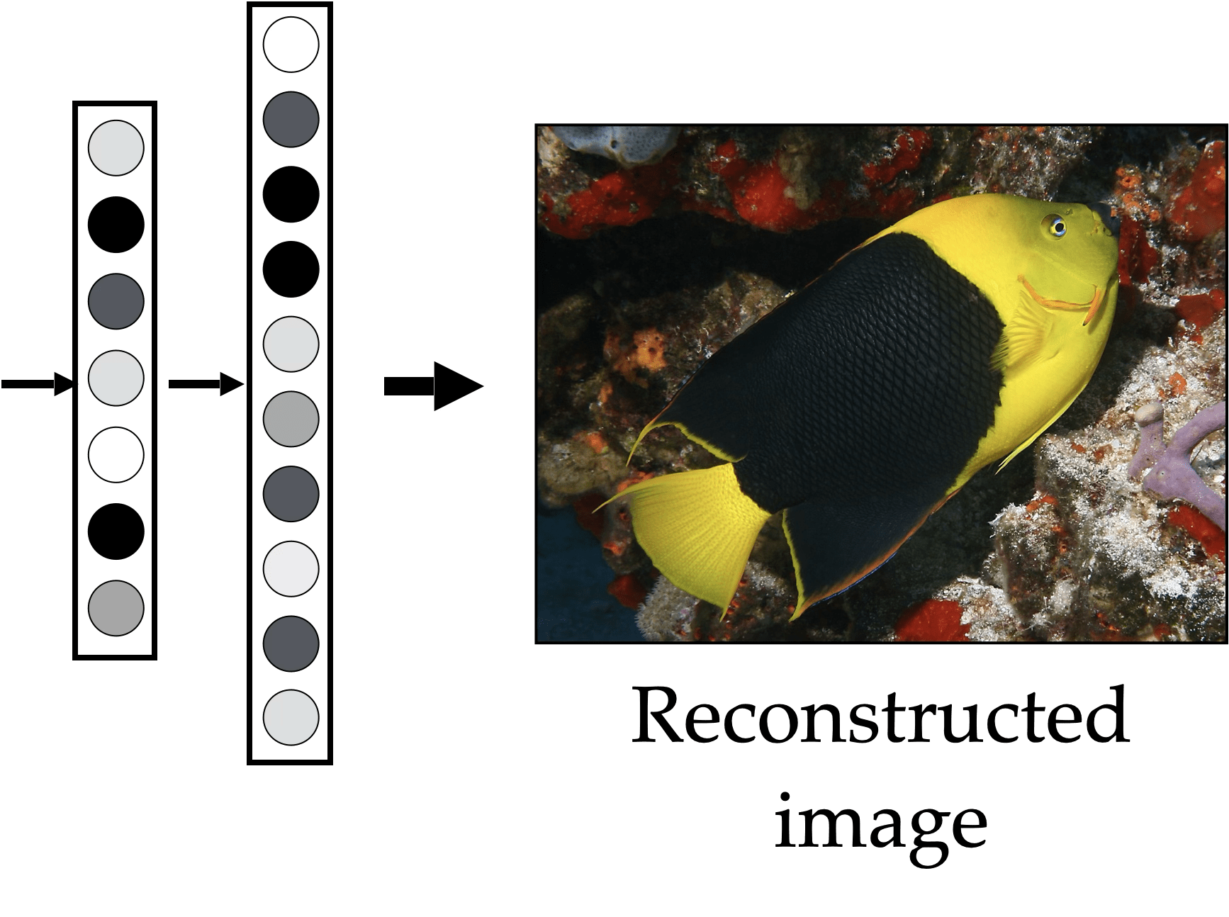
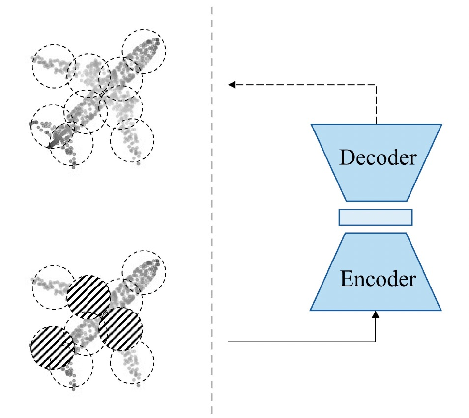
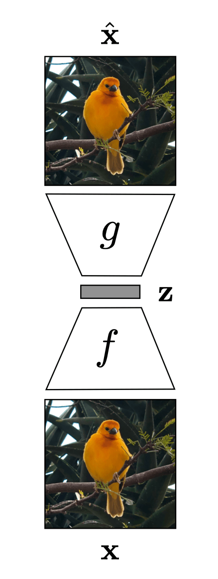
Auto-encoder
"What I cannot create, I do not understand." Feynman
[images credit: visionbook.mit.edu]
compact representation/embedding
Auto-encoder
encoder
decoder
bottleneck
Auto-encoder
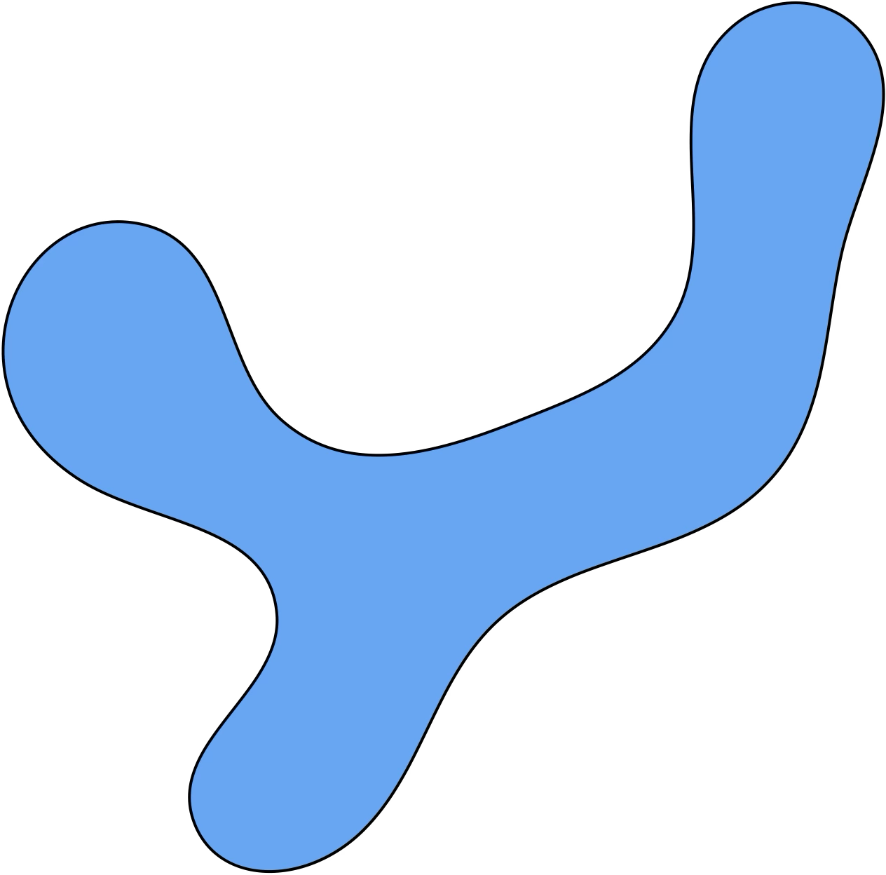
Data space:
(high dimensional, irregular)
Encoder
Decoder
Representation space
(low dimensional, regular)
[Typically, encoders can serve as a translator to get "good representations", whereas decoders can serve as "generative models"]
[Vincent et al, Extracting and composing robust features with denoising autoencoders, ICML 08]
But it's easy to "cheat" with auto-encoders
[Steck 20, Zhang et al 17]
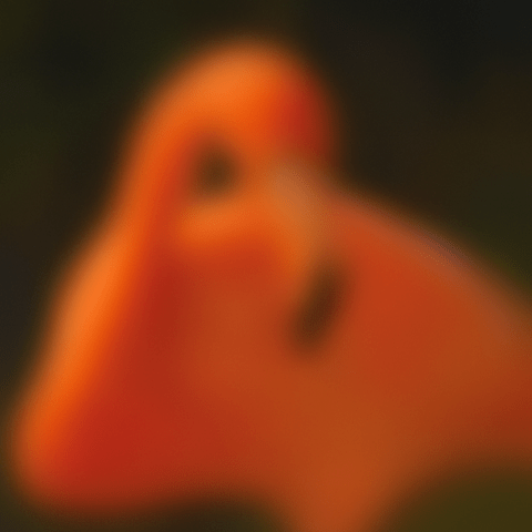

decoder

encoder
the reconstruction error is fine
but not very useful
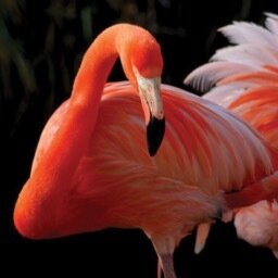
Unsupervised Learning (feature reconstruction)
Features
Reconstructed Features
$$x$$
$$\hat{x}$$
$$\hat{x}$$
$${x}$$
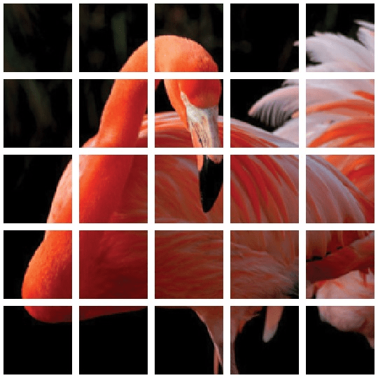
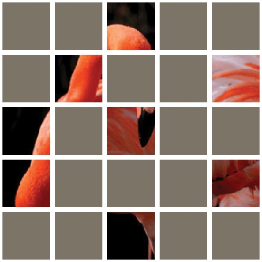
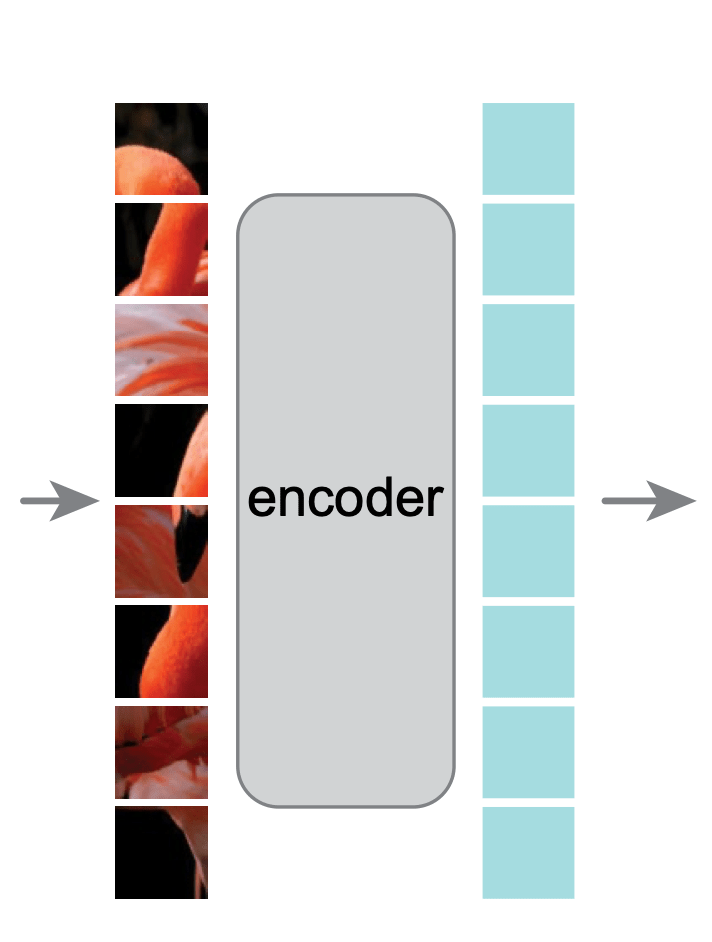
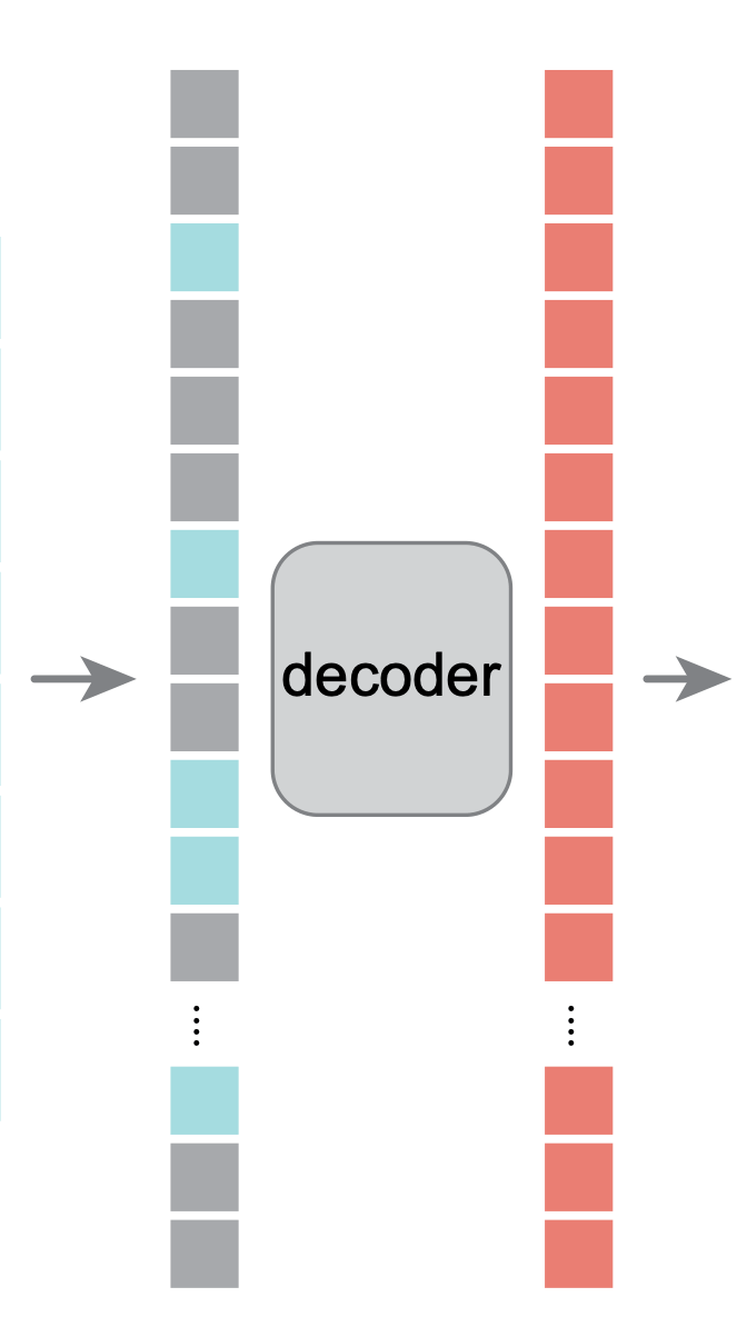
Self-supervised Learning (partial feature reconstruction)


Partial
Features
Other Partial Features
Harder reconstruction, forces understanding.
Masked Auto-Encoder (Vision)
[He, et al. Masked Autoencoders Are Scalable Vision Learners, 2021]
Large Language Models (LLMs) are trained in this self-supervised way
- Scrape the internet for plain texts.
- Cook up “labels” (prediction targets) from these texts.
- Convert “unsupervised” problem into “supervised” setup.
"To date, the cleverest thinker of all time was Issac. "
feature
label
To date, the
cleverest
To date, the cleverest
thinker
To date, the cleverest thinker
was
To date, the cleverest thinker of all time was
Issac
Outline
- Neural networks are representation learners
- Auto-encoders
- Word embeddings
- (Some recent representation learning ideas)
[video edited from 3b1b]
Word embedding
dot-product similarity
[video edited from 3b1b]
dot-product similarity
For now, let's look at how good embeddings enable "soft" dictionary look-up:
dict_en2fr = {
  "apple" : "pomme",
  "banana": "banane",
  "lemon" : "citron"}
Good word embeddings space is equipped with sensible dot-product similarity
Key
Value
apple
pomme
\(:\)
banane
banana
\(:\)
citron
lemon
\(:\)
dict_en2fr = {
  "apple" : "pomme",
  "banana": "banane",
  "lemon" : "citron"}

query = "lemon"
output = dict_en2fr[query]
apple
pomme
banane
citron
banana
lemon
Key
Value
lemon
\(:\)
\(:\)
\(:\)
Query
Output
citron
dict_en2fr = {
  "apple" : "pomme",
  "banana": "banane",
  "lemon" : "citron"}

query = "orange"
output = dict_en2fr[query]
Python would complain. 🤯
orange
apple
pomme
banane
citron
banana
lemon
Key
Value
\(:\)
\(:\)
\(:\)
Query
Output
???
What if we run
What if we run
But we can probably see the rationale behind this:
Query
Key
Value
Output
orange
apple
\(:\)
pomme
banana
\(:\)
banane
lemon
\(:\)
citron
dict_en2fr = {
  "apple" : "pomme",
  "banana": "banane",
  "lemon" : "citron"}

query = "orange"
output = dict_en2fr[query]
0.1
pomme
0.1
banane
0.8
citron
+
+
0.1
pomme
0.1
banane
0.8
citron
+
+
via these merging percentages [0.1 0.1 0.8] made sense
We put (query, key, value) in "good" embeddings in our human brain
such that "merging" the values
Query
Key
Value
Output
orange
apple
\(:\)
pomme
0.1
pomme
0.1
banane
0.8
citron
banana
\(:\)
banane
lemon
\(:\)
citron
+
+
orange
orange
0.1
pomme
0.1
banane
0.8
citron
+
+
apple
banana
lemon
orange
0.8
0.1
0.1
pomme
banane
citron
+
+
very roughly, the attention mechanism in transformers automates this process.
apple
banana
lemon
orange
orange
orange
Query
Key
Value
Output
orange
apple
\(:\)
pomme
banana
\(:\)
banane
lemon
\(:\)
citron
orange
orange
pomme
banane
citron
0.1
pomme
0.1
banane
0.8
citron
+
+
0.1
pomme
0.1
banane
0.8
citron
+
+
dot-product similarity
softmax
0.1
0.1
0.8
1. compare query and key for merging percentages:
apple
banana
lemon
orange
softmax
orange
orange
Query
Key
Value
Output
orange
apple
\(:\)
pomme
0.1
pomme
0.1
banane
0.8
citron
banana
\(:\)
banane
lemon
\(:\)
citron
+
+
orange
orange
pomme
banane
citron
+
+
0.1
0.1
0.8
0.8
0.1
0.1
pomme
banane
citron
+
+
2. then output merged values
1. compare query and key for merging percentages:
many more bells and whistles, we'll discuss next week
Outline
- Neural networks are representation learners
- Auto-encoders
- Word embeddings
- (Some recent representation learning ideas)
- 1. masking: reconstruction
- 2. contrastive: similarity
- 3. multi-modality: alignment
[Section slides partially adapted from Kaiming He, Philip Isola, and Andrew Owens]
[Zhang, Isola, Efros, ECCV 2016]
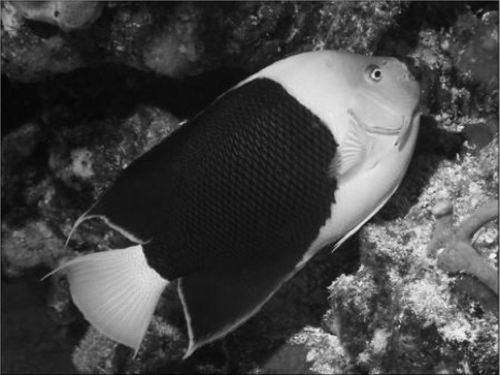
e.g. masking channels
1. Masking
predict color from gray-scale
[Zhang, Isola, Efros, ECCV 2016]
1. Masking
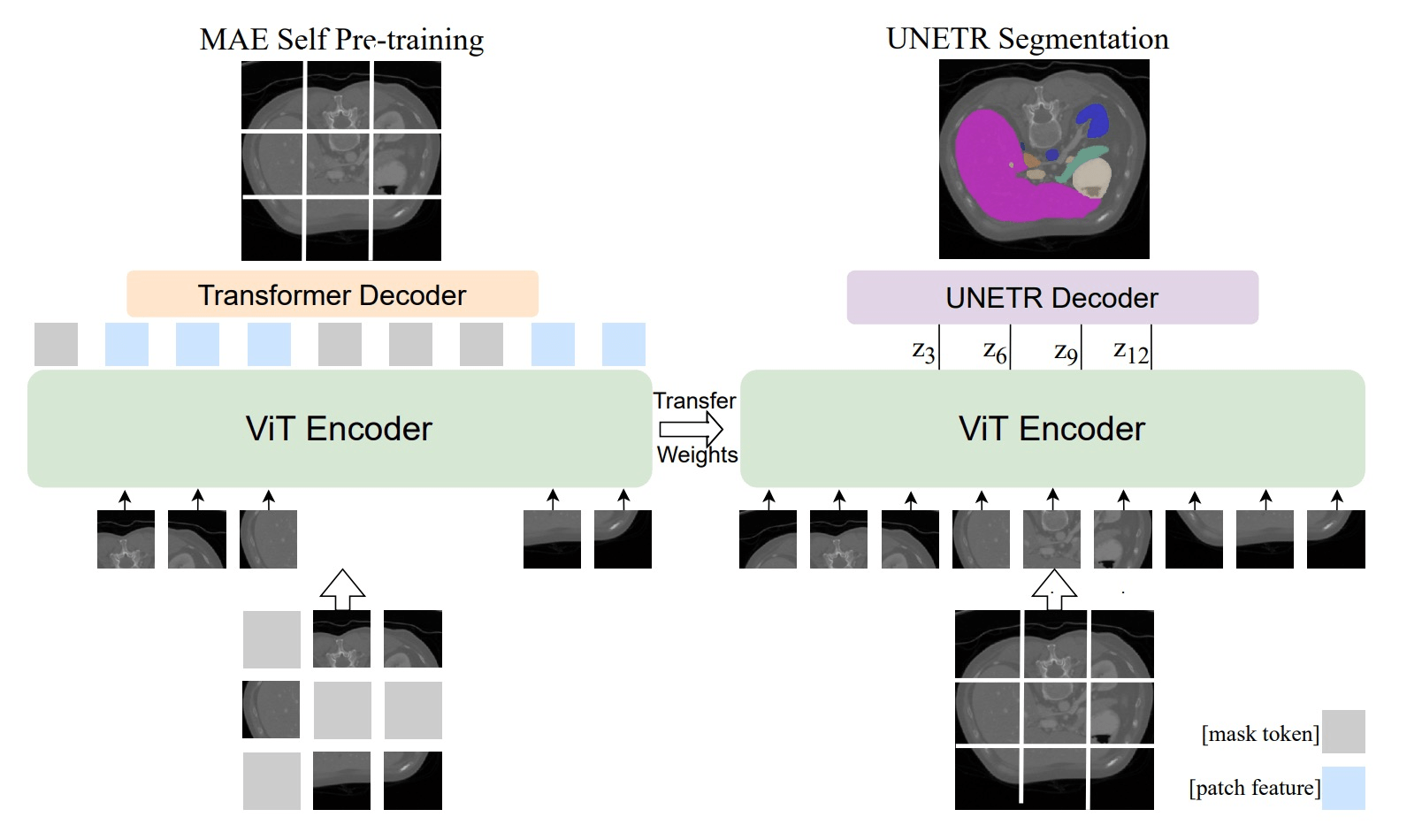
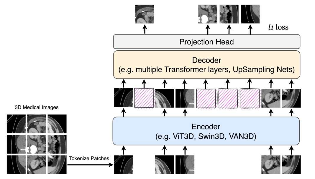
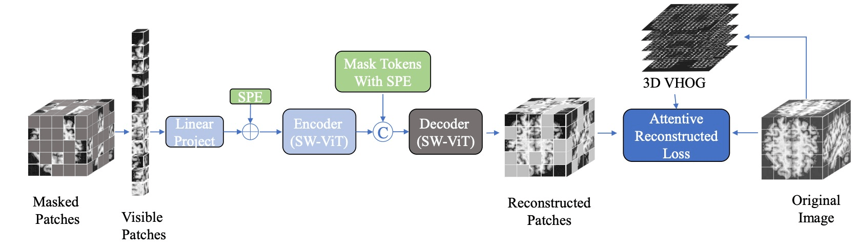
e.g. medical imaging
[Zhou+,'22; Chen+,'22; Huang+,'22; An+,'22]
1. Masking
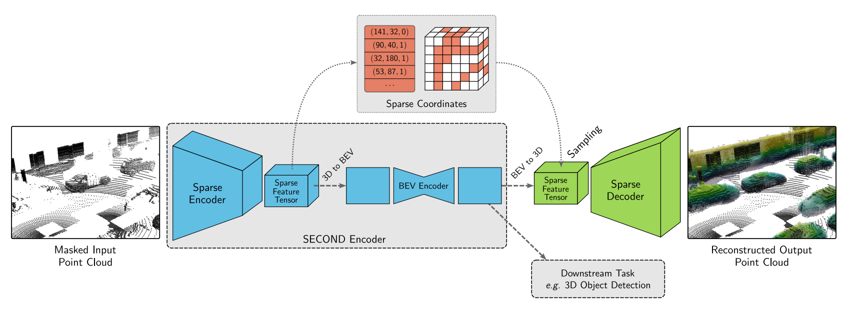
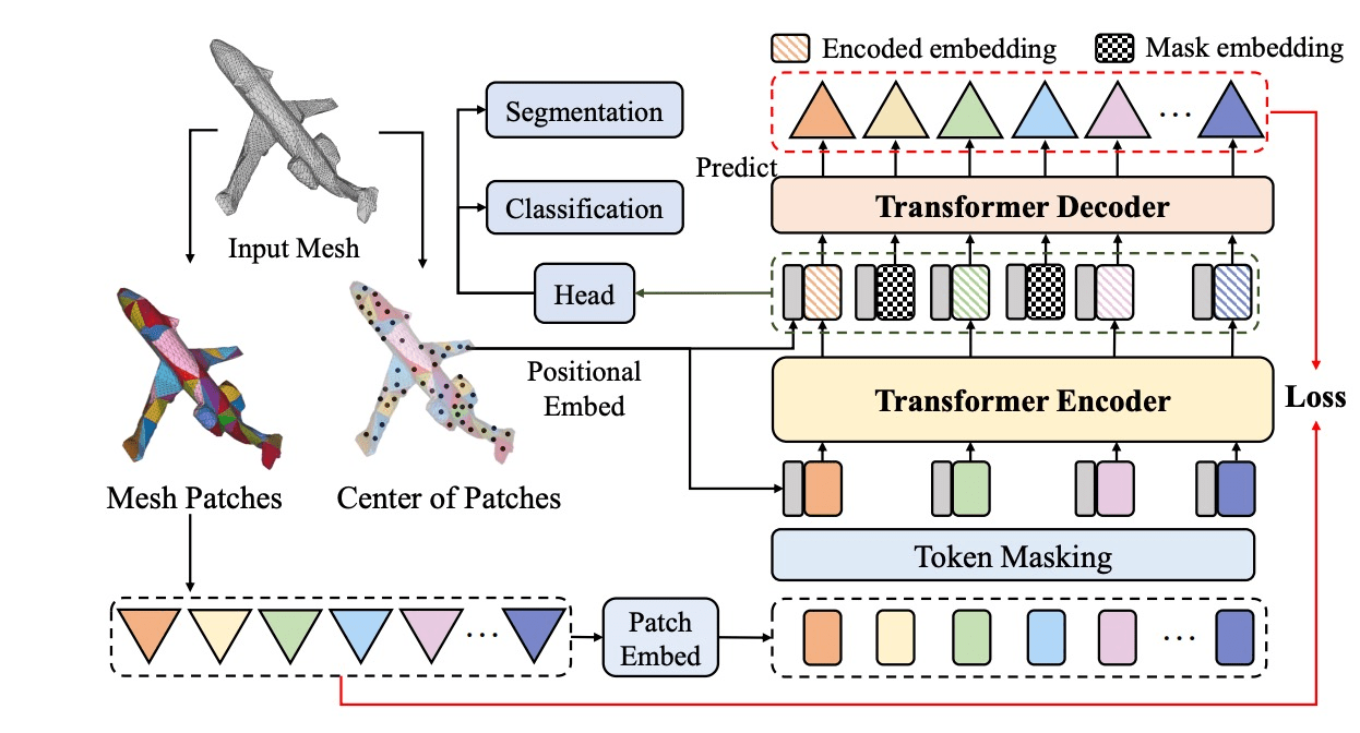
e.g. 3d geometry
[Pang+, '22; Liang+, '22; Min+, '22; Krispel+, '22]
1. Masking
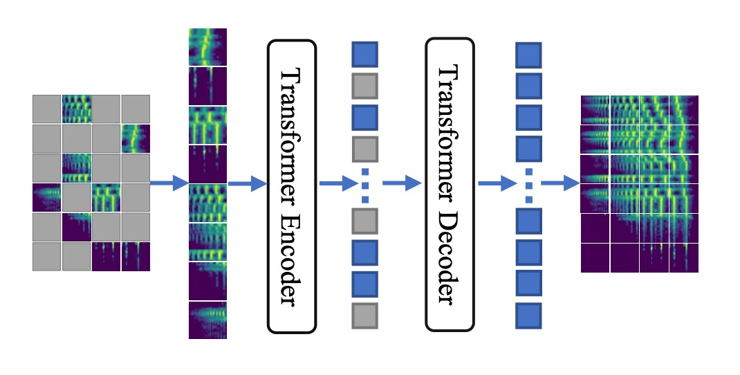
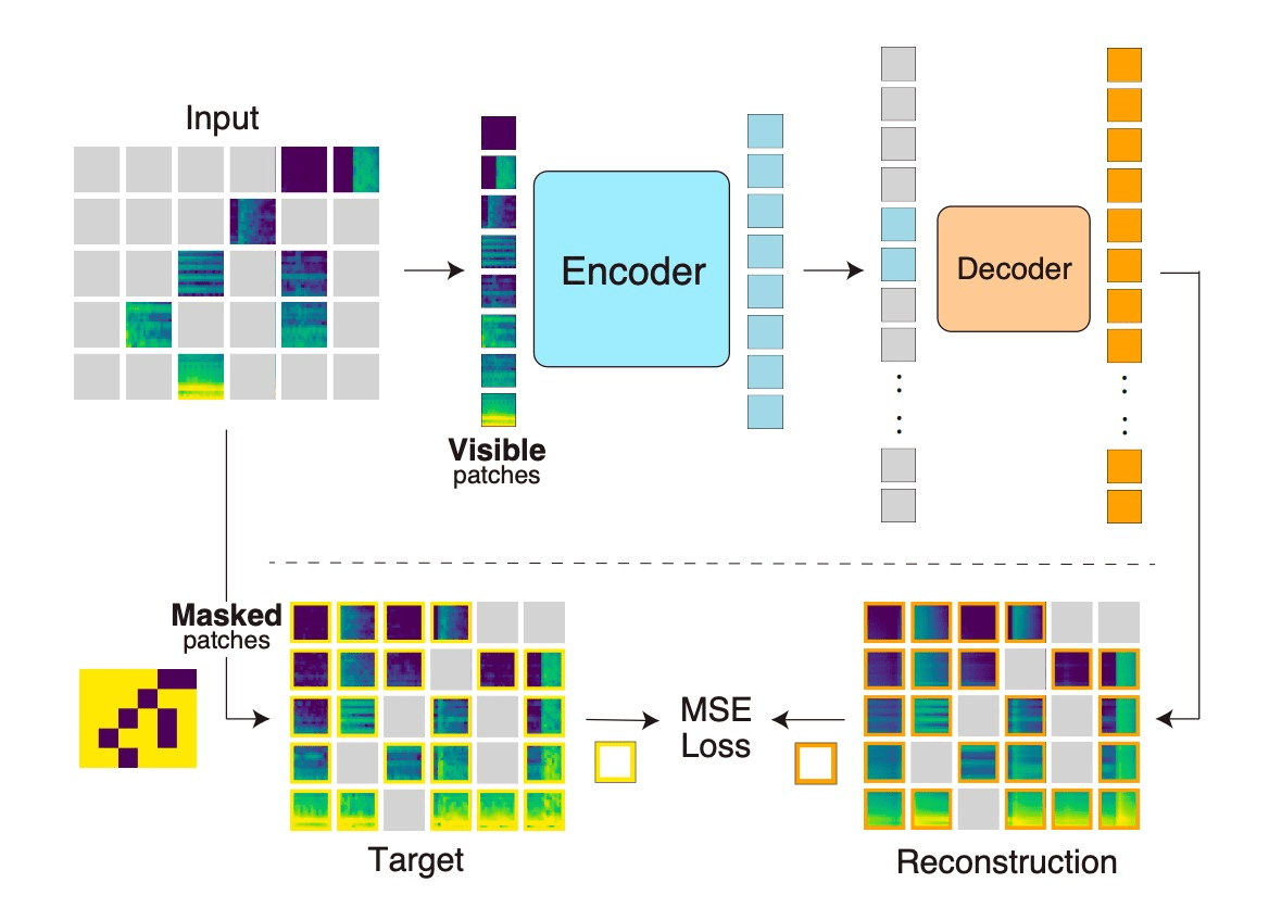
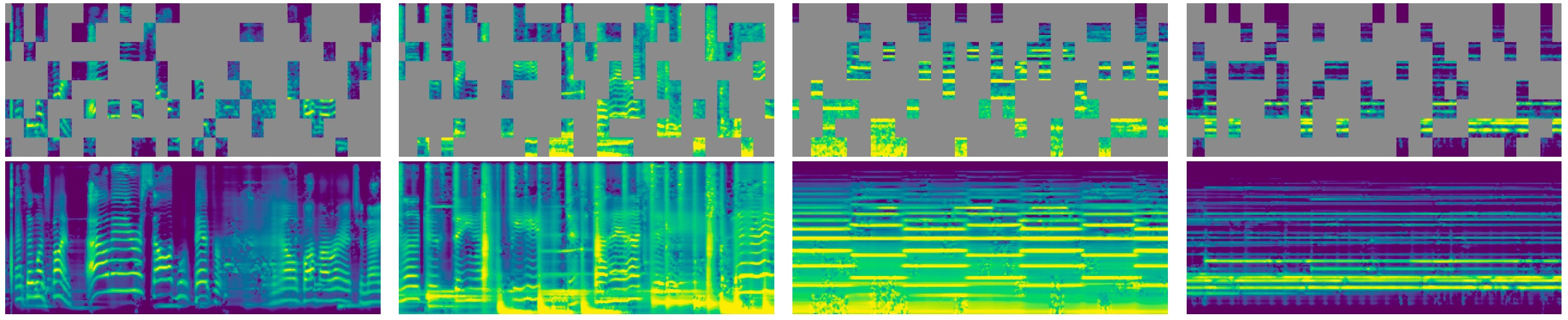
e.g. audio
[Baade+, '22; Chong+, '22; Niizumi, '22; Huang+, '22]
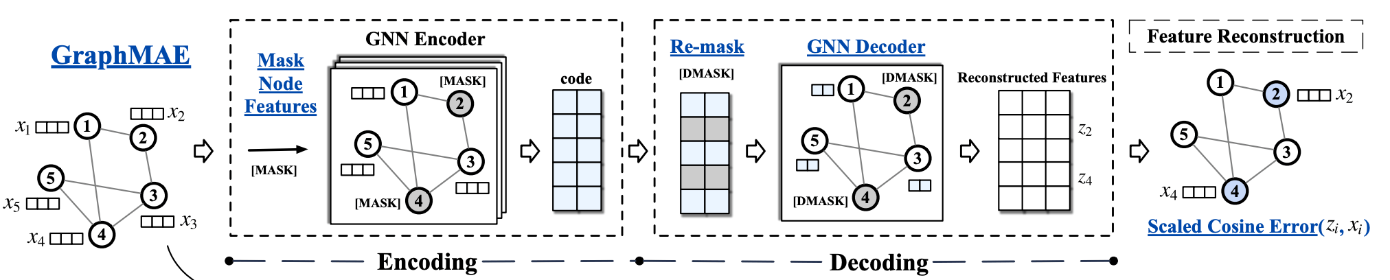
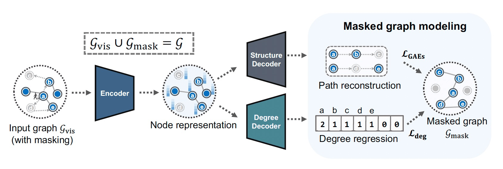
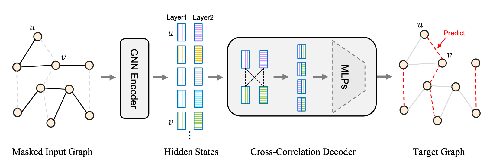
e.g. graphs
[Tan+, '22; Zhang+, '22; Hou+, '22; Li+, '22]
e.g. robotics
[Xiao+, '22; Radosavovic+, '22; Seo+, '22;]
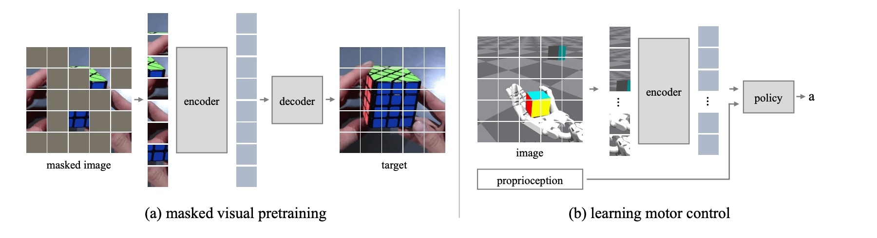
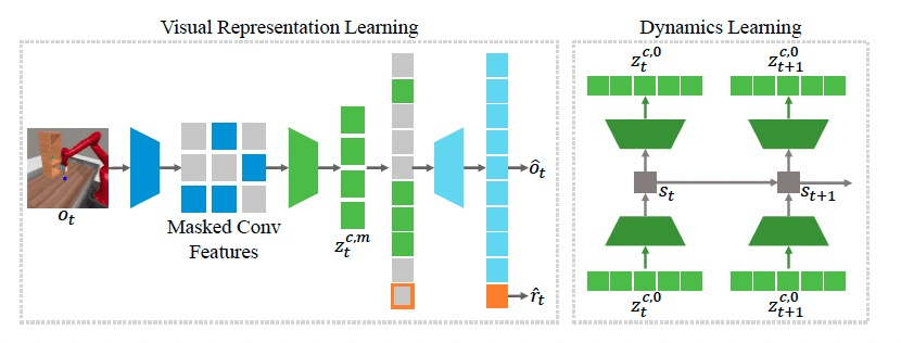
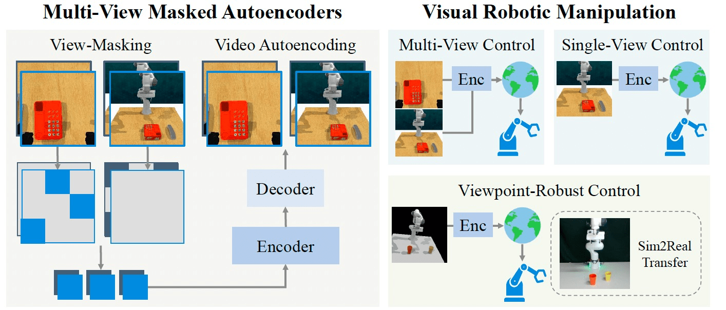
1. Masking
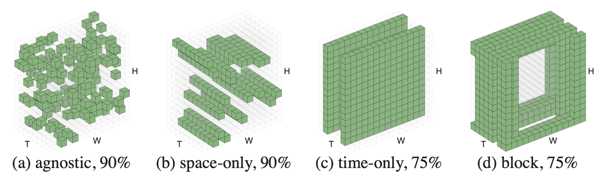
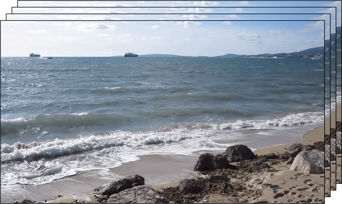
[Feichtenhofer, et al., "Masked Autoencoders As Spatiotemporal Learners", NeurIPS 2022]
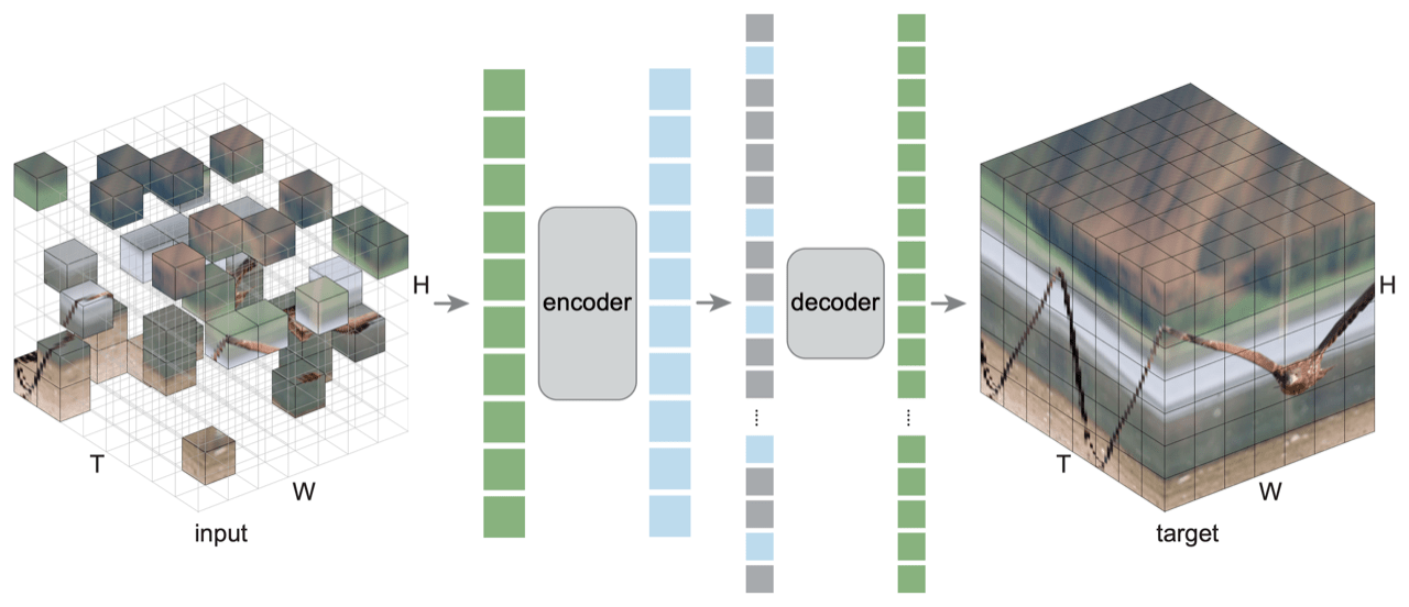
1. Masking
[Feichtenhofer, et al., "Masked Autoencoders As Spatiotemporal Learners", NeurIPS 2022]
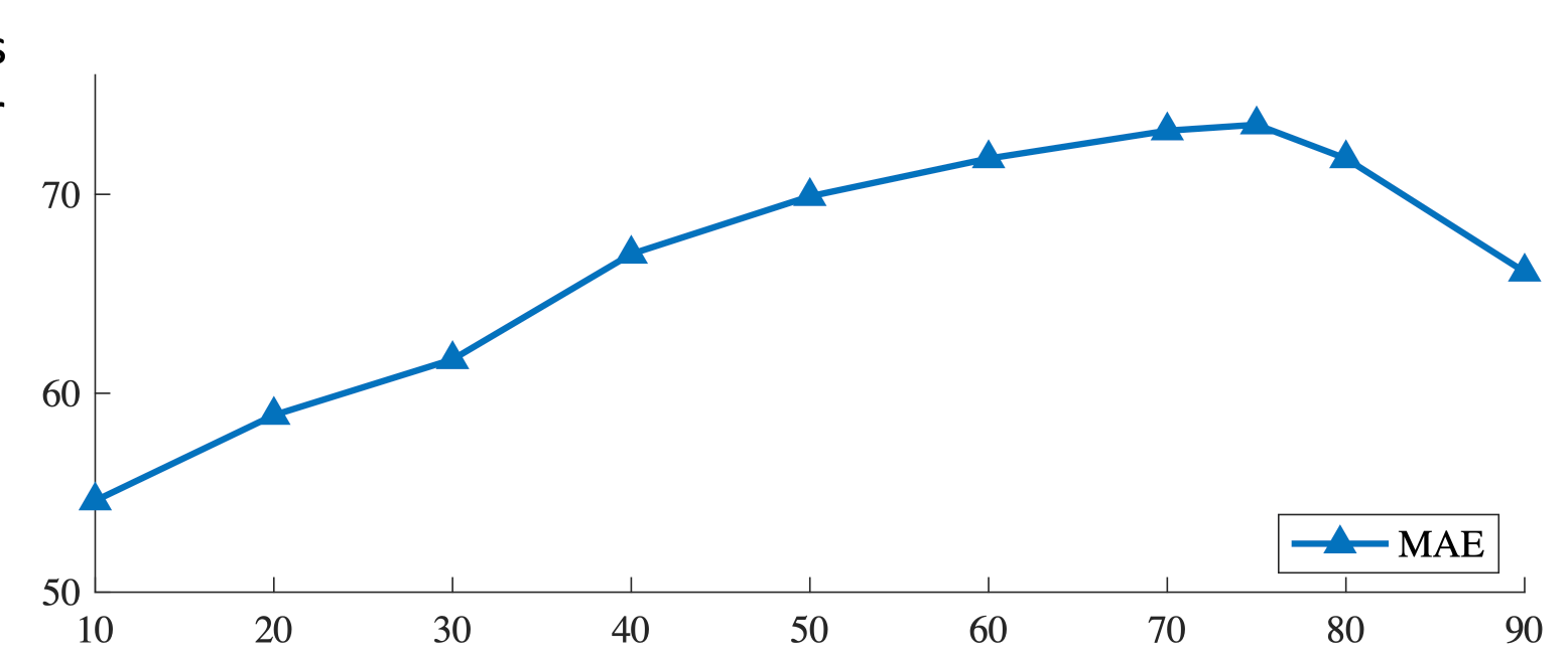
[He, et al. Masked Autoencoders Are Scalable Vision Learners, 2021]
masking ratio
transfer accuracy
masking 75% is
optimal for images
1. Masking
95% masked
98% masked
Similar empirical studies shows 15% as optimal for languages, and 95% for videos
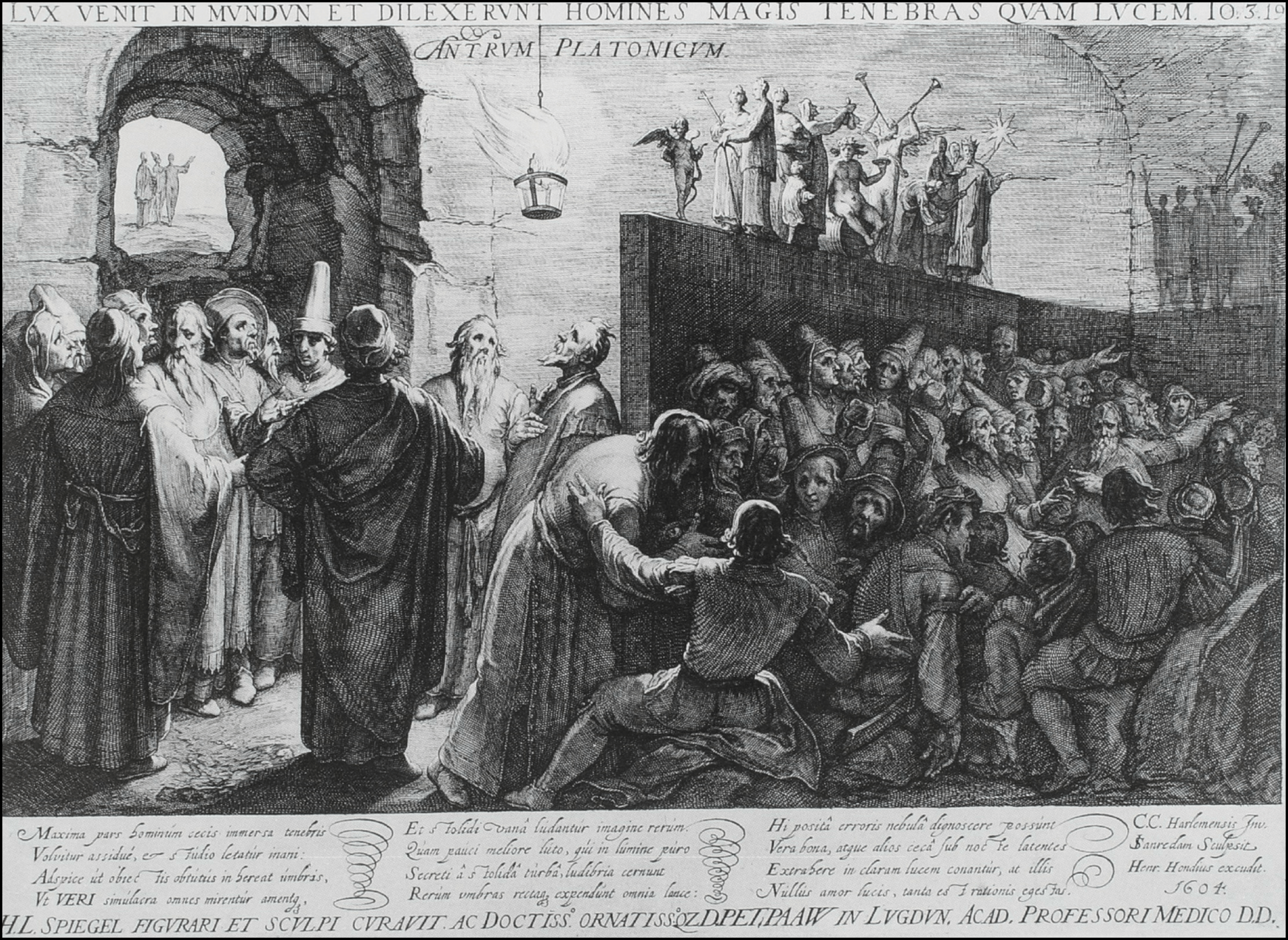

The allegory of the cave
2. Contrastive learning

[images credit: visionbook.mit.edu]
2. Contrastive learning
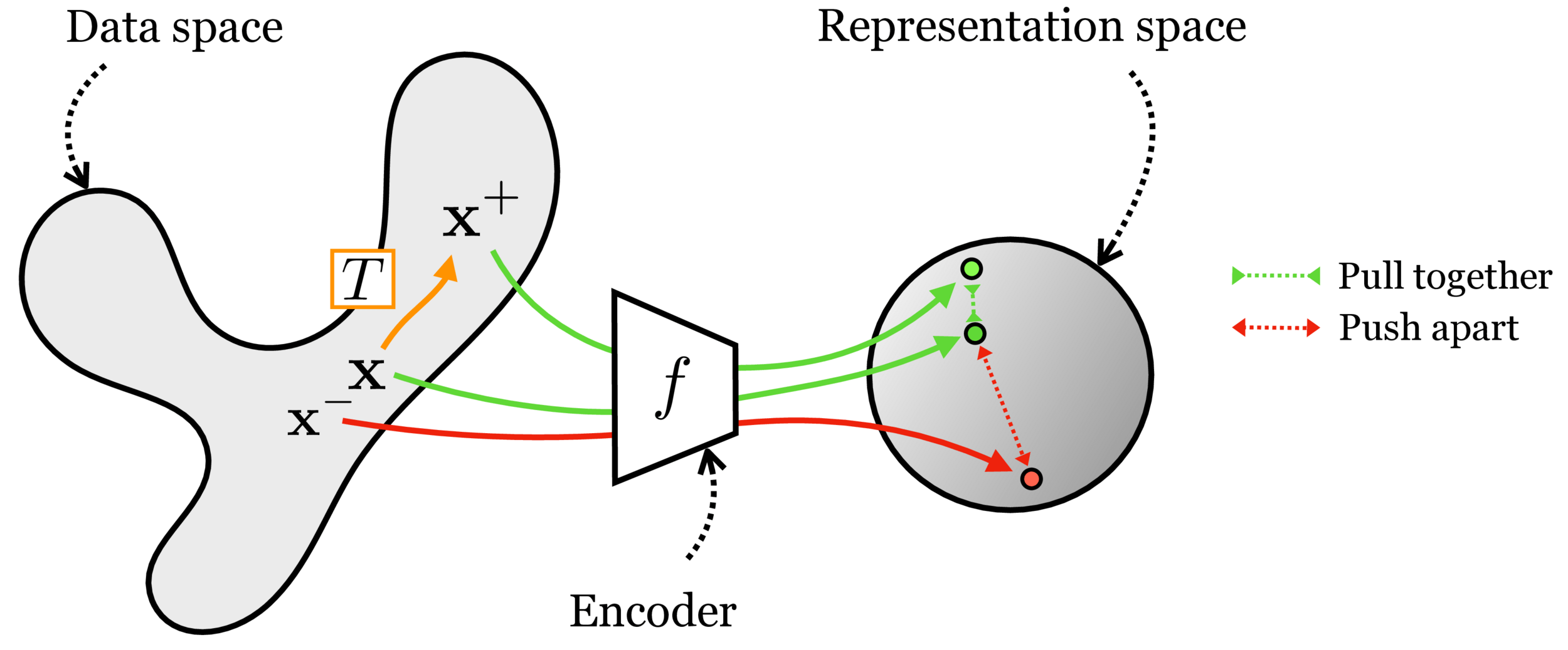
[images credit: visionbook.mit.edu]
2. Contrastive learning

[Chen, Kornblith, Norouzi, Hinton, ICML 2020]
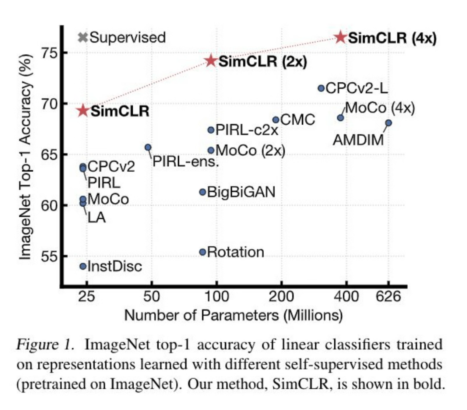
SimCLR animation
2. Contrastive learning
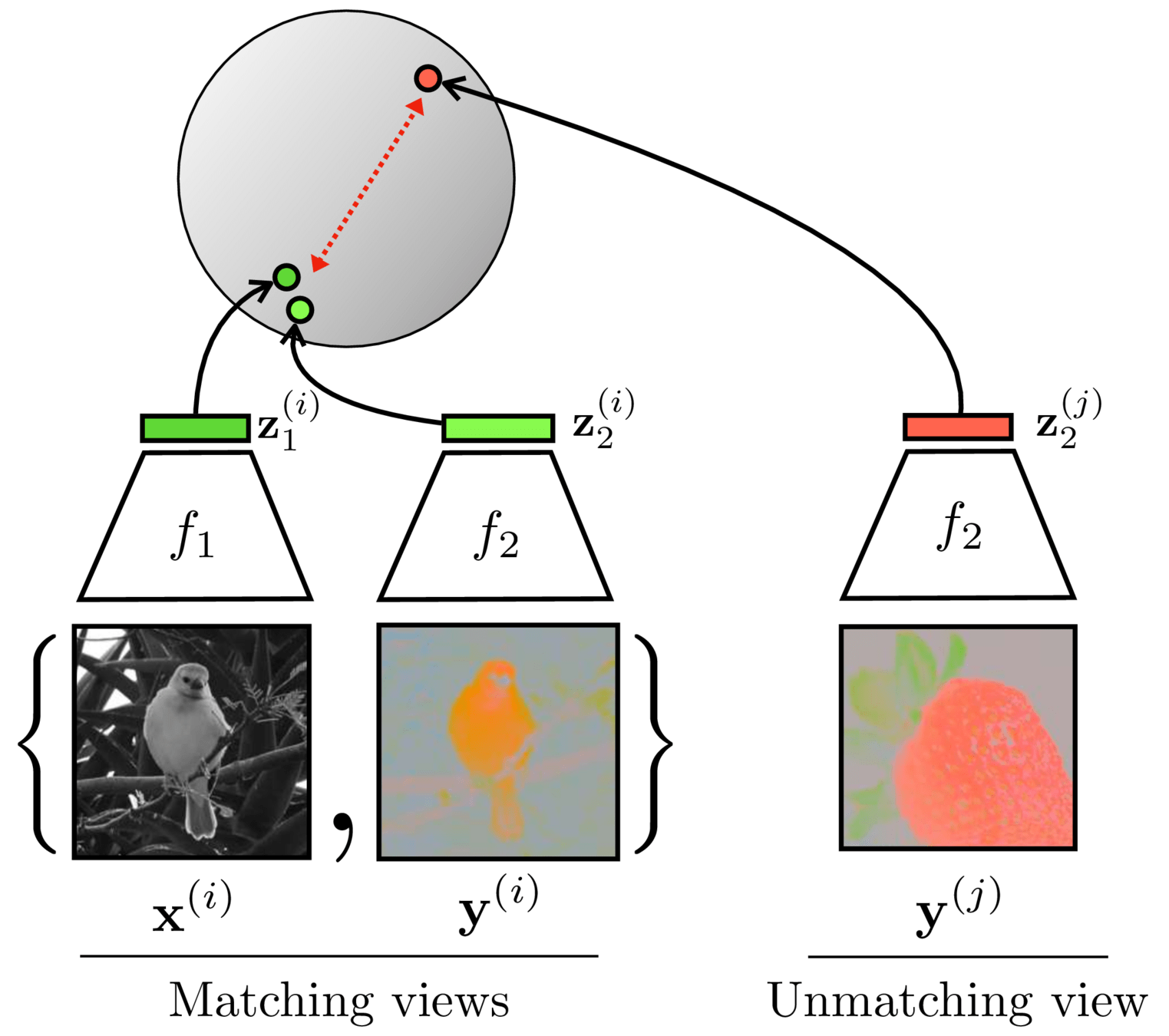
3. Multi-modality
[images credit: visionbook.mit.edu]
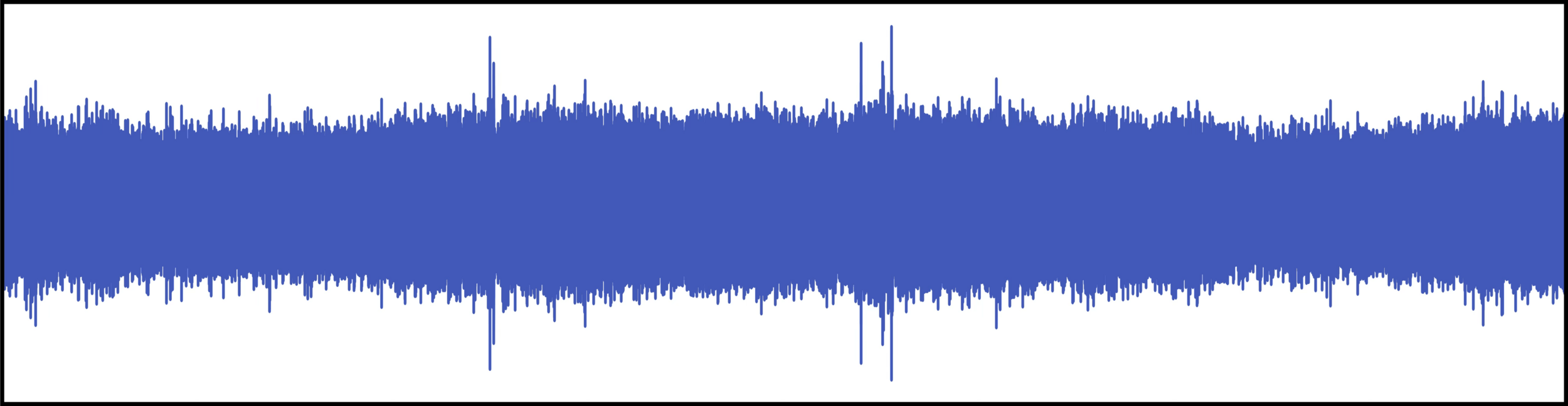
[Owens et al, Ambient Sound Provides Supervision for Visual Learning, ECCV 2016]
e.g. video, audio, images
[Owens et al, Ambient Sound Provides Supervision for Visual Learning, ECCV 2016]
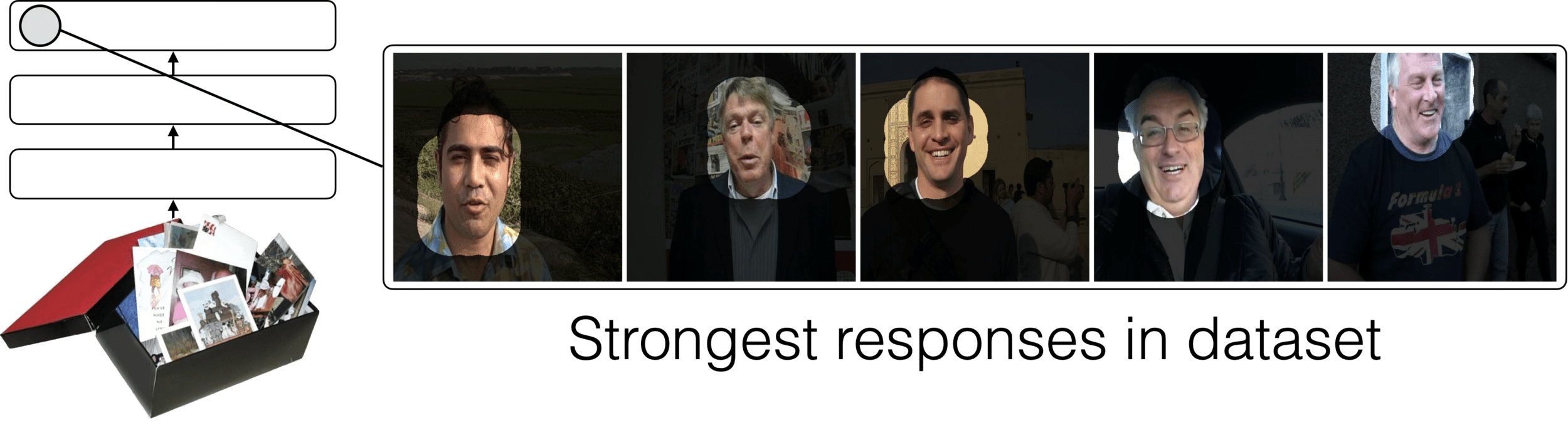
What did the model learn?
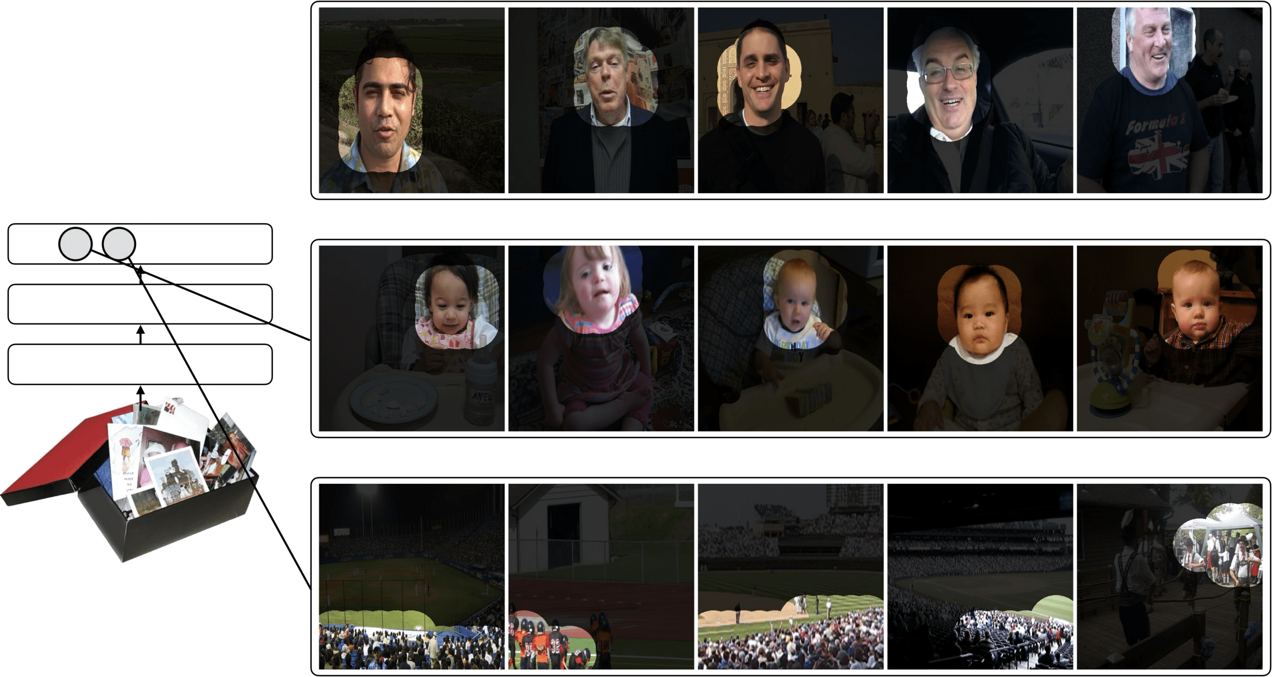
[Owens et al, Ambient Sound Provides Supervision for Visual Learning, ECCV 2016]
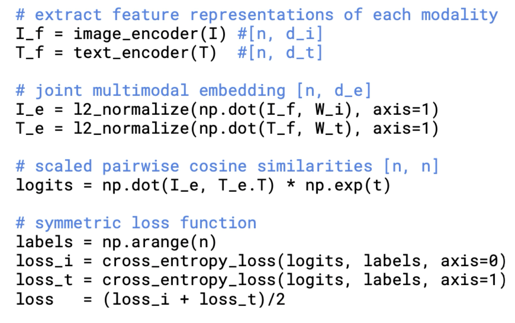
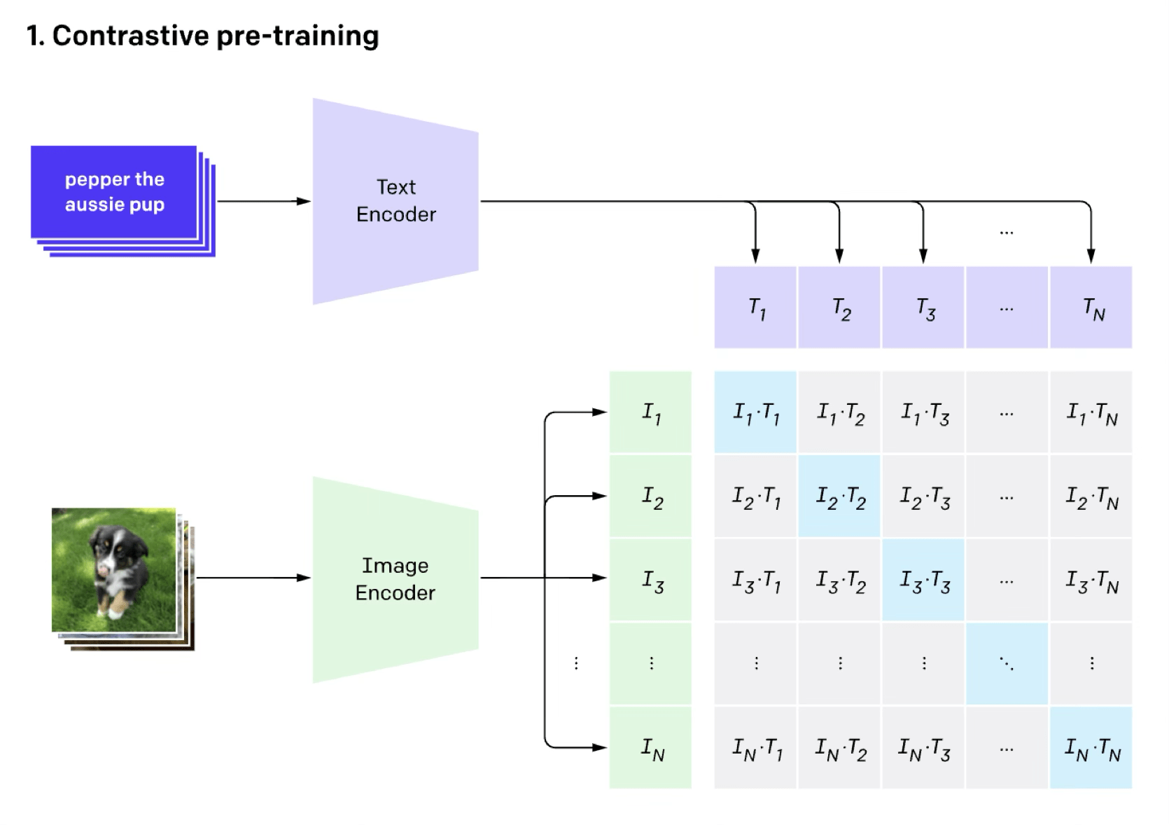
e.g. image classification (done in the contrastive way)
[Radford et al, Learning Transferable Visual Models From Natural Language Supervision, ICML, 2011]
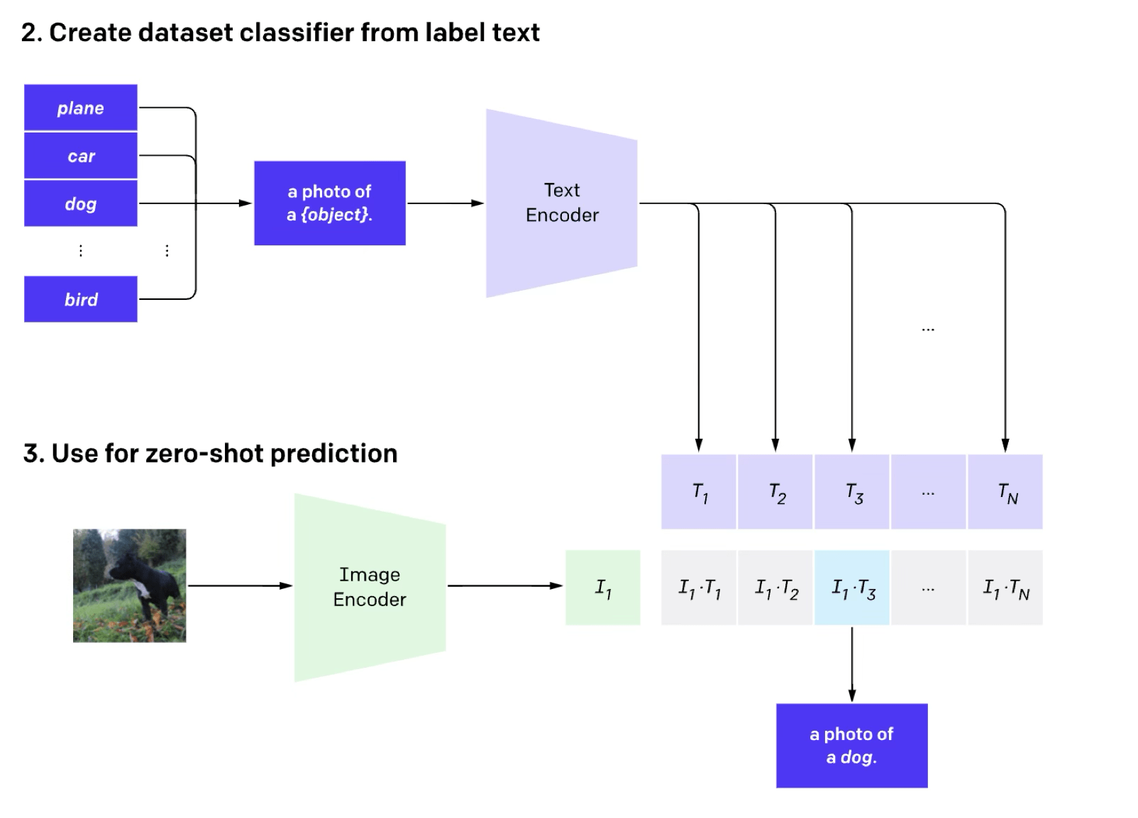
e.g. image classification (done in the contrastive way)
[Radford et al, Learning Transferable Visual Models From Natural Language Supervision, ICML, 2011]
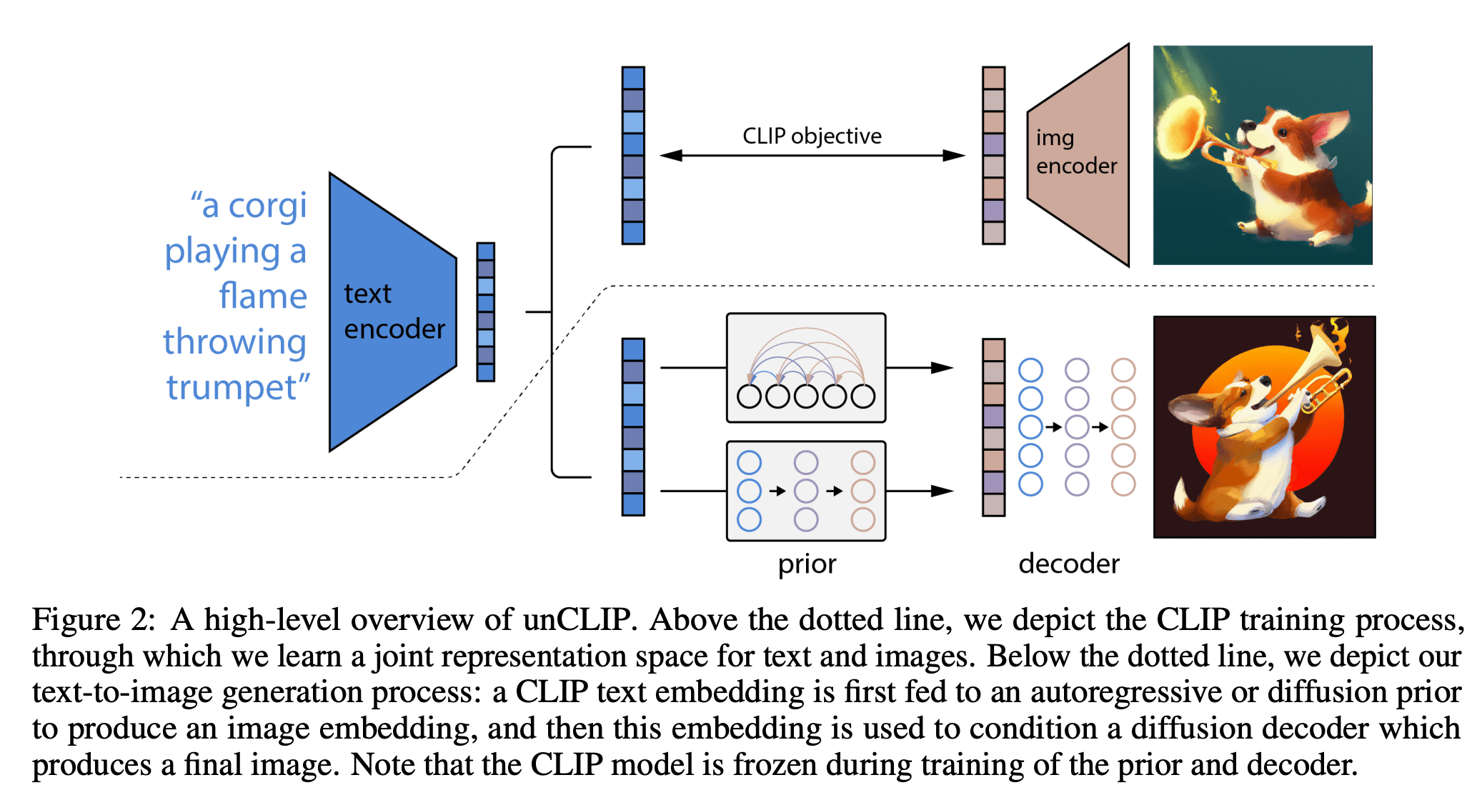
[https://arxiv.org/pdf/2204.06125.pdf]
e.g Dall-E: text-image generation
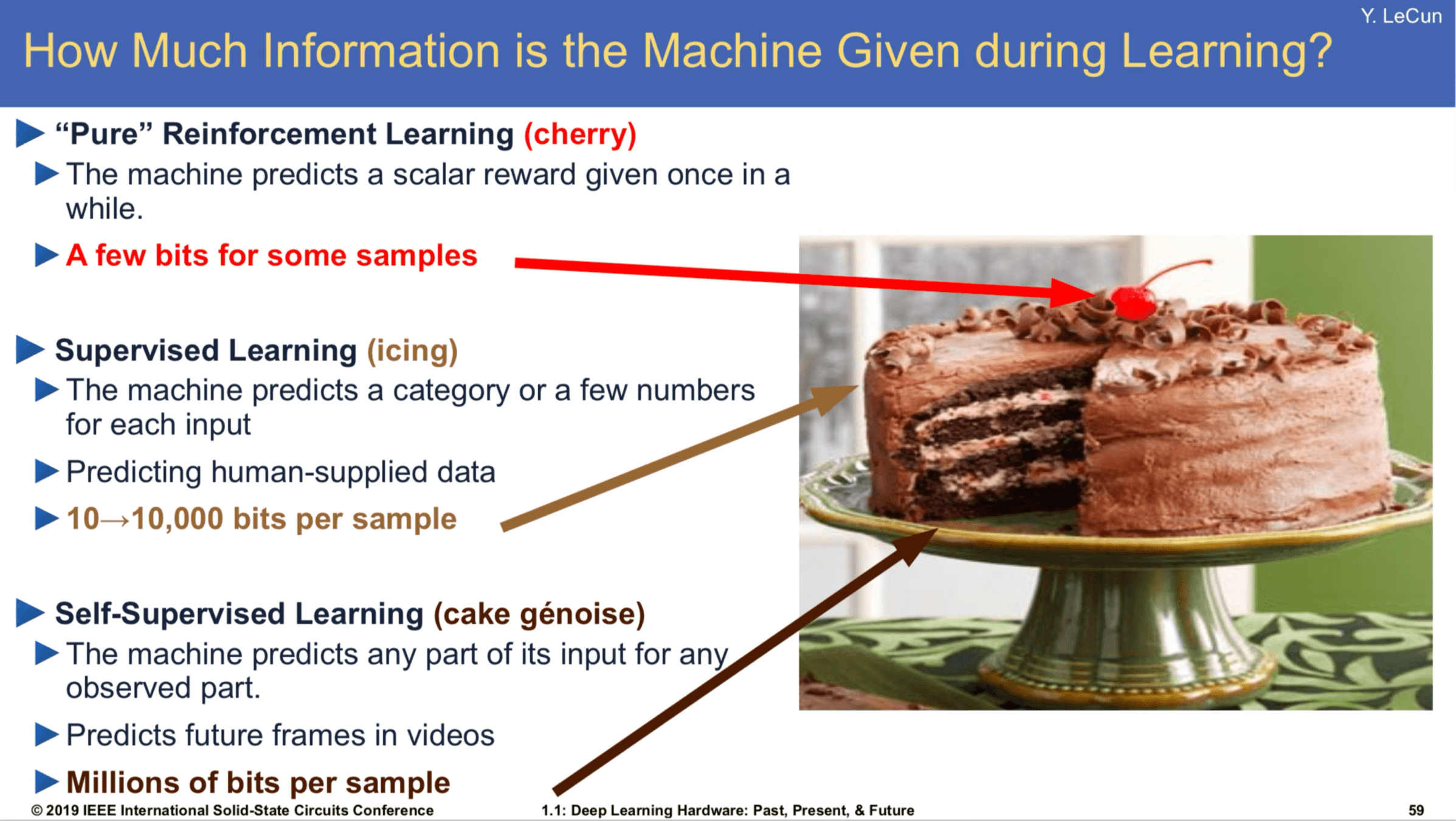
[Slide Credit: Yann LeCun]
Summary
- We looked at the mechanics of NN. Today we see they learn representations, just like our brains do.
- This is useful because representations transfer — they act as prior knowledge that enables quick learning on new tasks.
- Representations can also be learned without labels, e.g. as we do in unsupervised, or self-supervised learning. This is great since labels are expensive and limiting.
- Without labels there are many ways to learn representations:
- representations as compressed codes, auto-encoder with bottleneck
- (representations that are predictive of their context)
- (representations that are shared across sensory modalities)
Thanks!
We'd love to hear your thoughts.
Auto-encoder
Training Data
loss/objective
hypothesis class
A model
\(f\)
\(m<d\)
[images credit: visionbook.mit.edu]
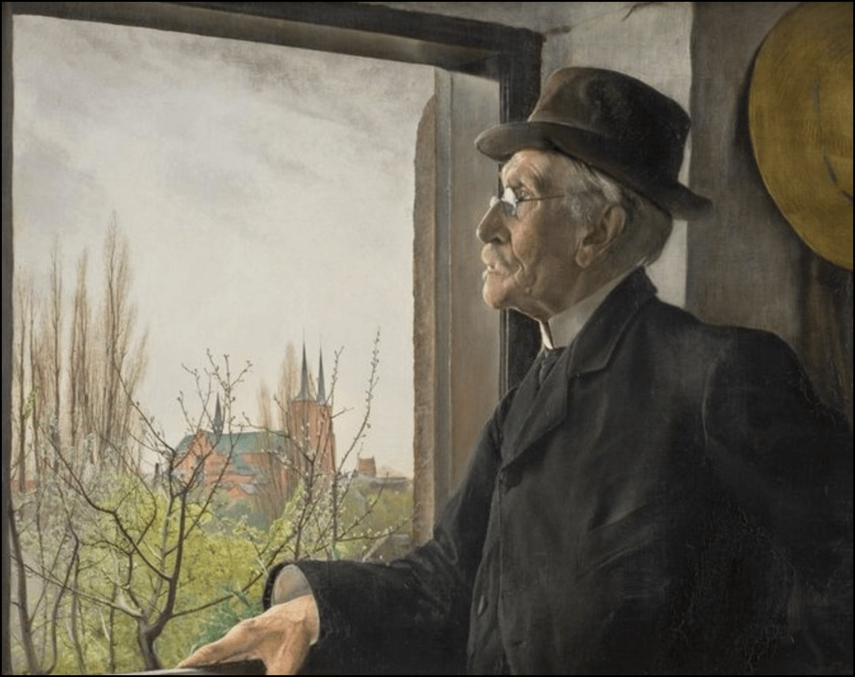
"I stand at the window and see a house, trees, sky. Theoretically I might say there were 327 brightnesses and nuances of colour. Do I have "327"? No. I have sky, house, and trees.”
— Max Wertheimer, 1923
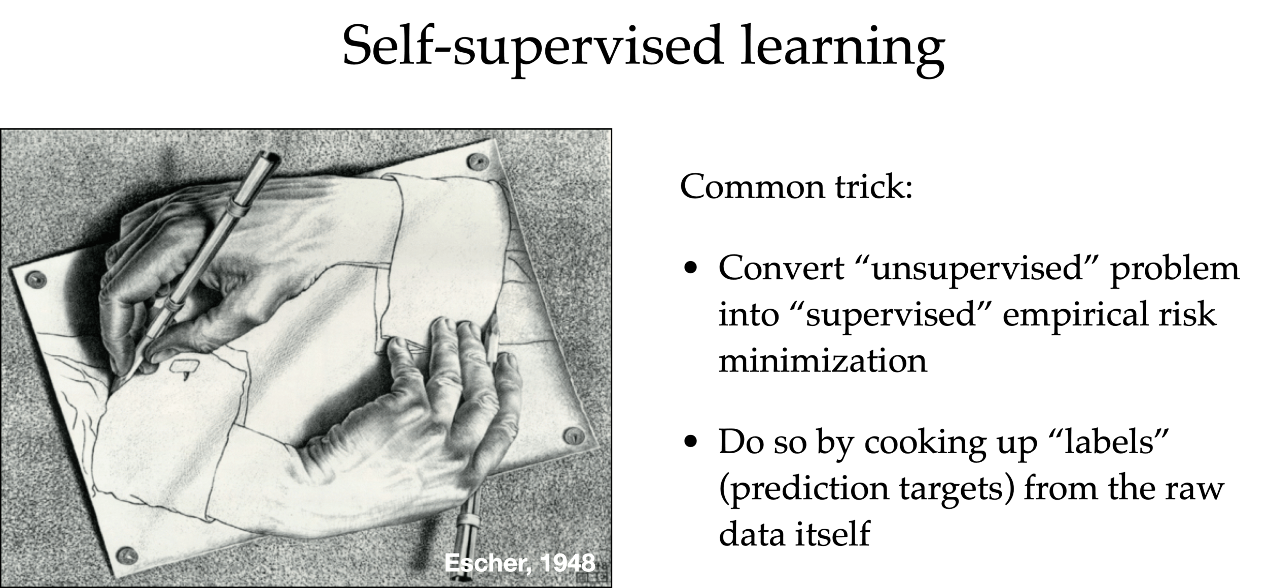
Self-supervised learning
Common trick:
- Convert “unsupervised” problem into “supervised” setup
- Do so by cooking up “labels” (prediction targets) from the raw data itself — called pretext task
"Good"
Representation
Unsupervised Learning
Training Data
$$\{x^{(1)}\}$$
$$\{x^{(2)}\}$$
$$\{x^{(3)}\}$$
$$\ldots$$
Learner
Supervised Learning
Algorithm
🧠⚙️
hypothesis class
loss function
hyperparameters
\(\mathcal{D}_\text{train}\)
\(\left\{\left(x^{(1)}, y^{(1)}\right), \dots, \left(x^{(n)}, y^{(n)}\right)\right\}\)
[video edited from 3b1b]
[video edited from 3b1b]
Query
Key
Value
Output
orange
apple
\(:\)
pomme
banana
\(:\)
banane
lemon
\(:\)
citron
0.1
pomme
0.1
banane
0.8
citron
+
+
0.1
pomme
0.1
banane
0.8
citron
+
+
and this merging percentage also made sense
We implicitly assumed the (query, key, value) are 'good' embeddings.
such that the "merging" made sense
apple
banana
lemon
orange
orange
orange
dot-product similarity
very roughly, the attention mechanism does exactly this kind of "soft" look-up:
softmax
0.1
0.1
0.8
Query
Key
Value
Output
orange
apple
\(:\)
pomme
banana
\(:\)
banane
lemon
\(:\)
citron
orange
orange
apple
banana
lemon
orange
0.1
pomme
0.1
banane
0.8
citron
+
+
pomme
banane
citron
+
+
very roughly, the attention mechanism does exactly this kind of "soft" look-up:
Query
Key
Value
Output
orange
apple
\(:\)
pomme
0.1
pomme
0.1
banane
0.8
citron
banana
\(:\)
banane
lemon
\(:\)
citron
+
+
orange
orange
0.1
pomme
0.1
banane
0.8
citron
+
+
apple
banana
lemon
orange
apple
banana
lemon
orange
softmax
orange
orange
Query
Key
Value
Output
orange
apple
\(:\)
pomme
banana
\(:\)
banane
lemon
\(:\)
citron
orange
orange
pomme
banane
citron
0.1
pomme
0.1
banane
0.8
citron
+
+
pomme
banane
citron
+
+
very roughly, the attention mechanism does exactly this kind of "soft" look-up:
0.1
0.1
0.8
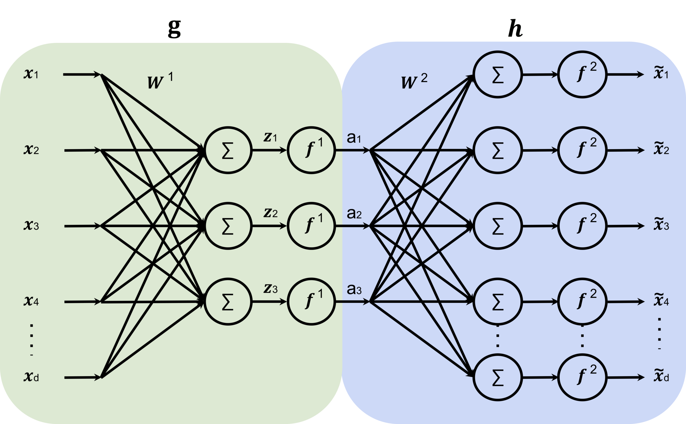
input \(x \in \mathbb{R^d}\)
output \(\tilde{x} \in \mathbb{R^d}\)
bottleneck
typically, has lower dimension than \(d\)
Masked Auto-Encoder (Language)
[Devlin, Chang, Lee, et al. 2019]
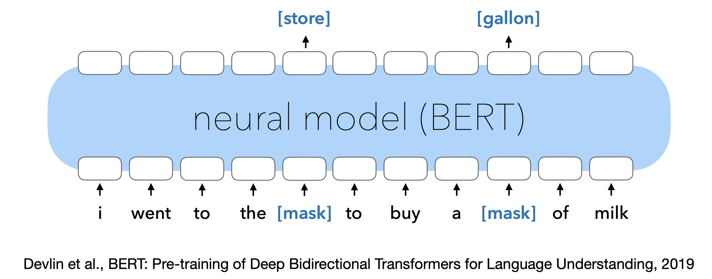
Same concept applies to text → masked words instead of masked pixels.
- masking strategies
- contrastive
- multi-modality