

Lecture 5: Features and Neural Networks I
Intro to Machine Learning

Recall:
step
multi-class
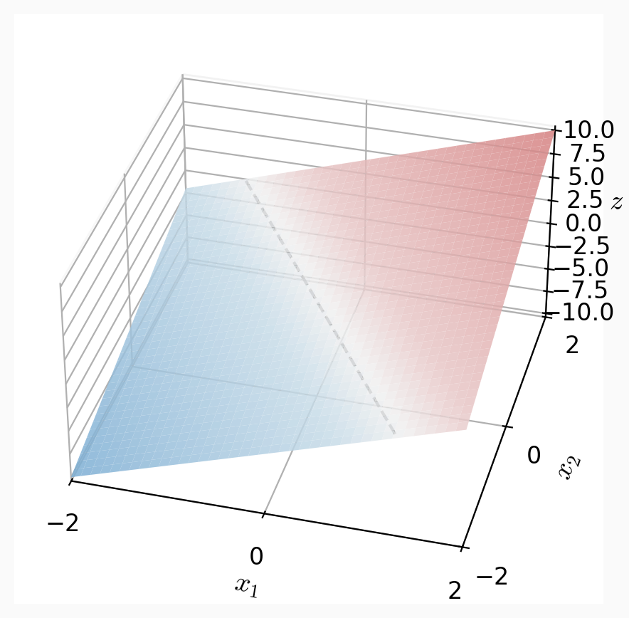
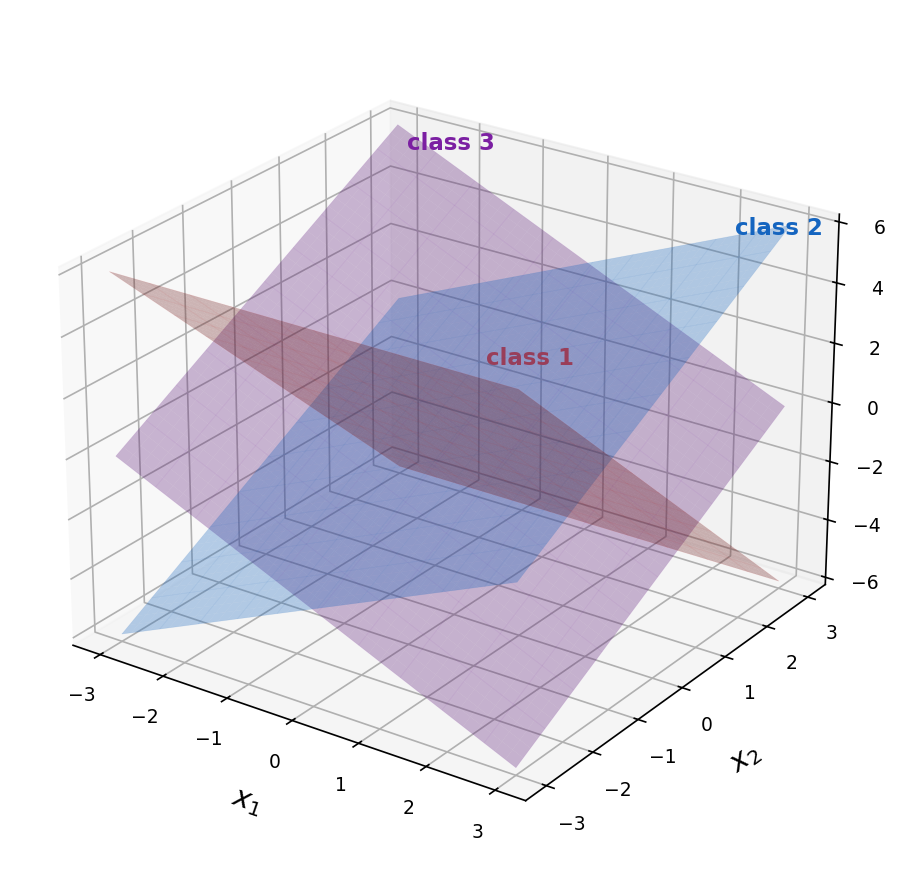
\(z = \theta^{\top} x+\theta_0\)
\(z = \theta^{\top} x+\theta_0\)
\(z_k = \theta_k^{\top} x+\theta_{0,k}\)
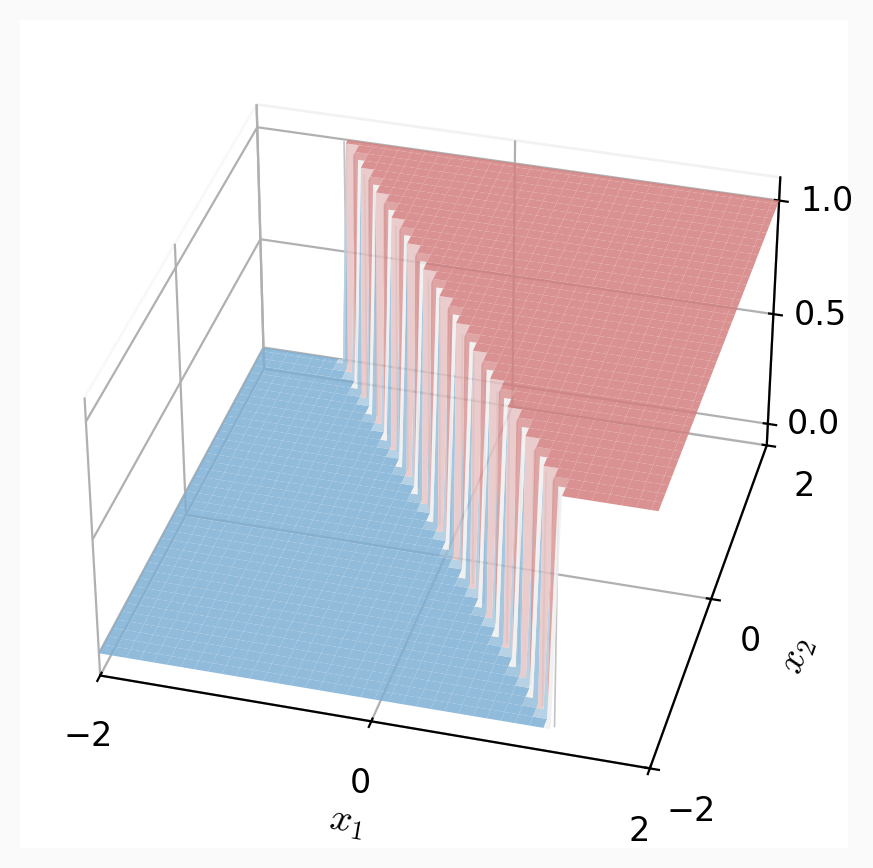
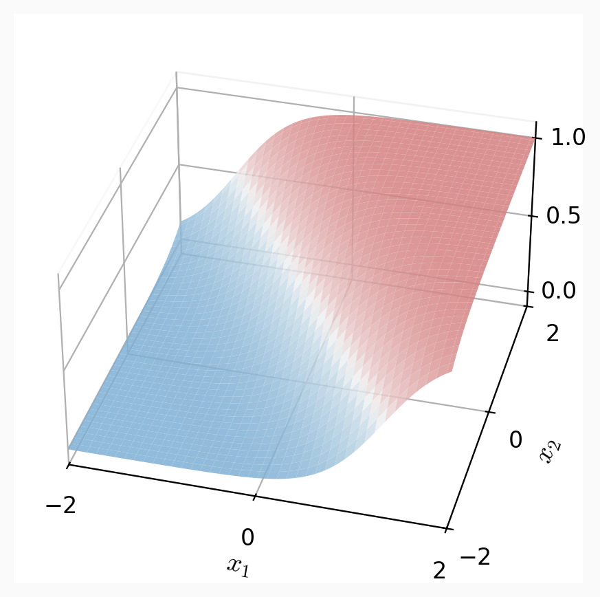
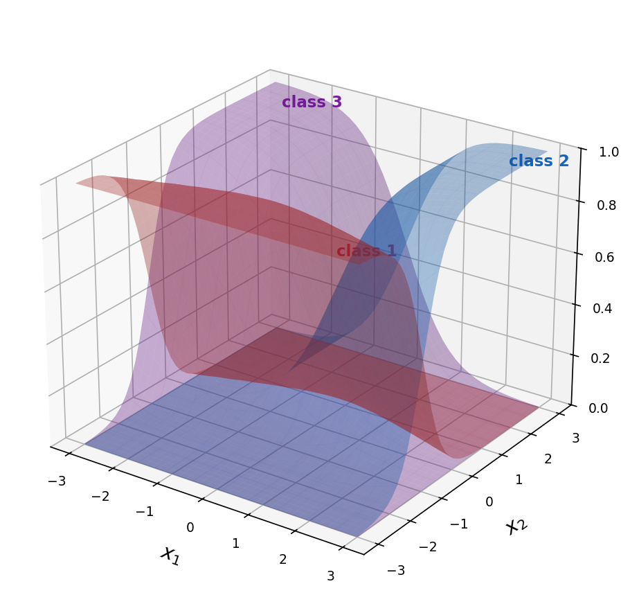
\(g = \text{step}(z)\)
\(g = \sigma(z)\)
\(g = \text{softmax}(z_1,\ldots,z_K)\)
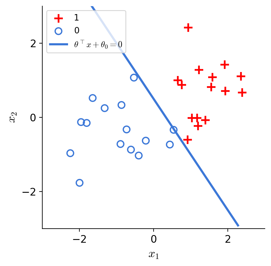
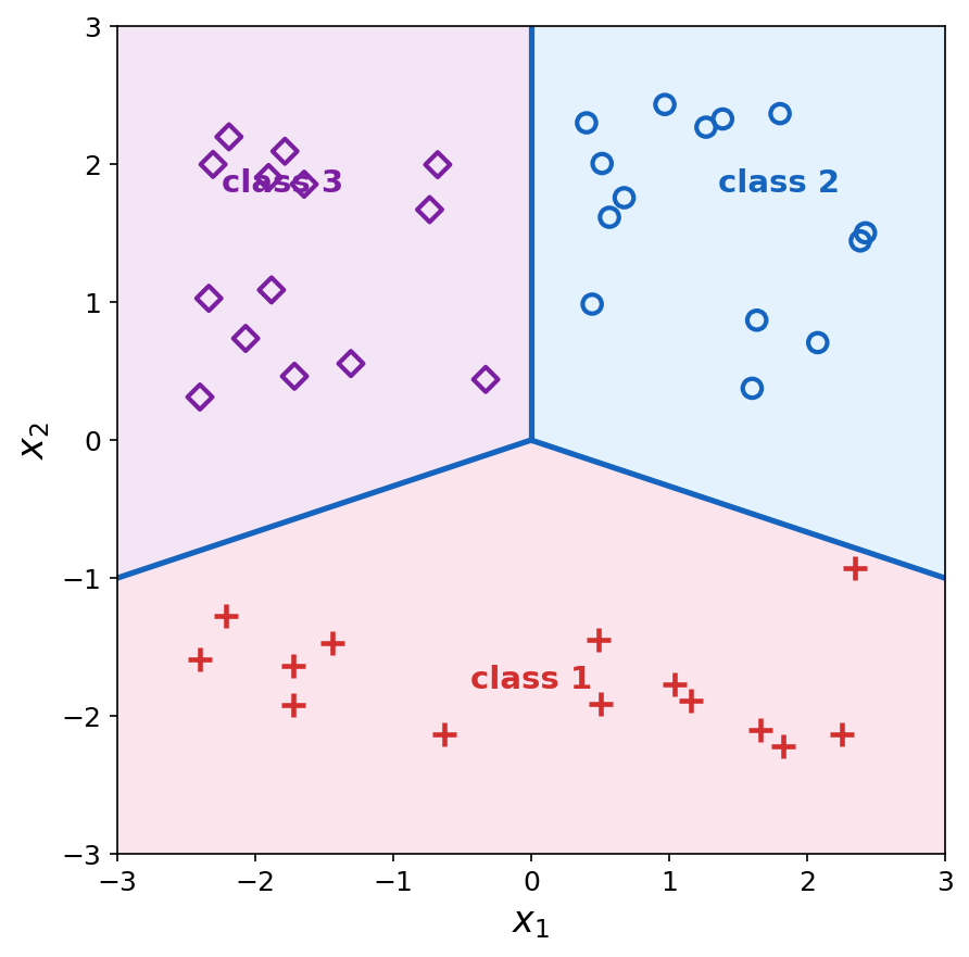
decision boundary is linear in \(x\)
logistic
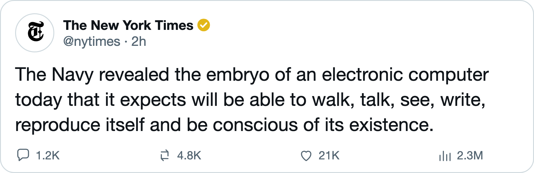
[mock-up post generated by Claude Opus 5.5, not real]
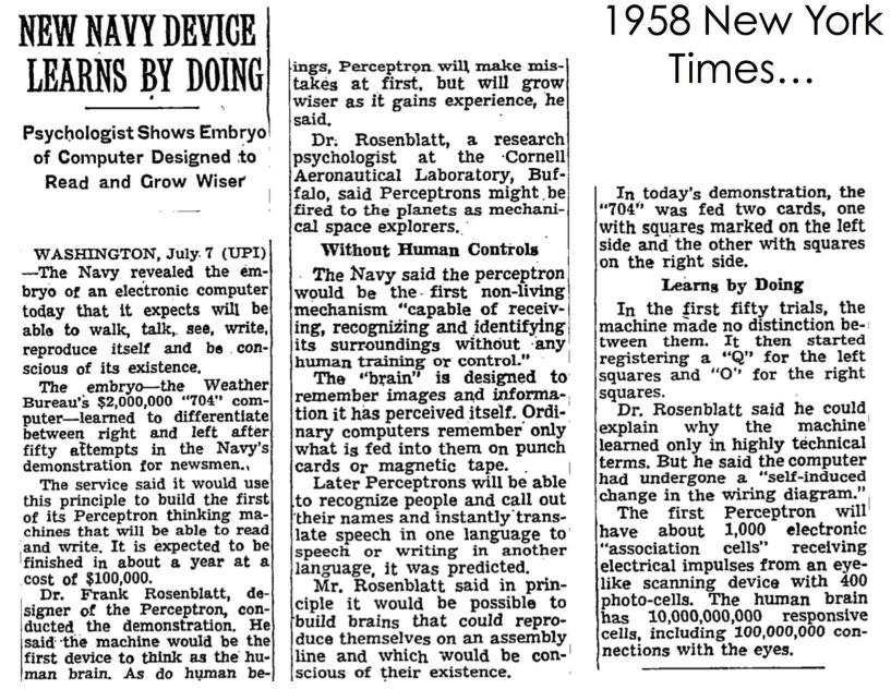
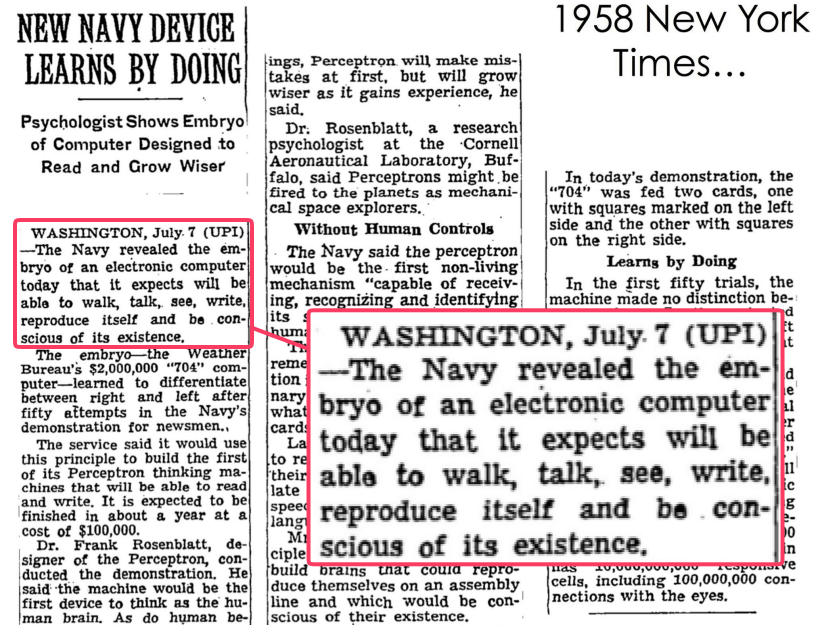
[real front-page of NY Times]
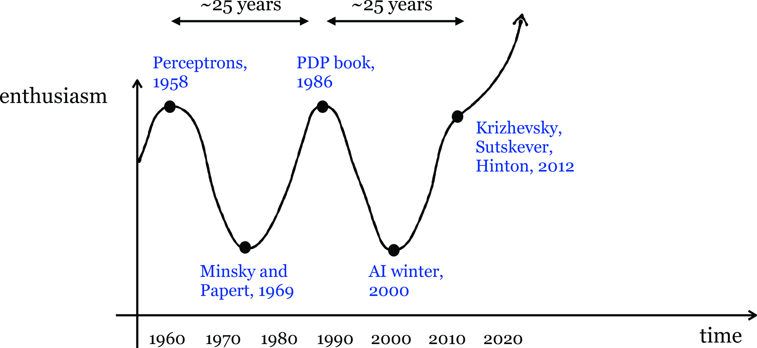
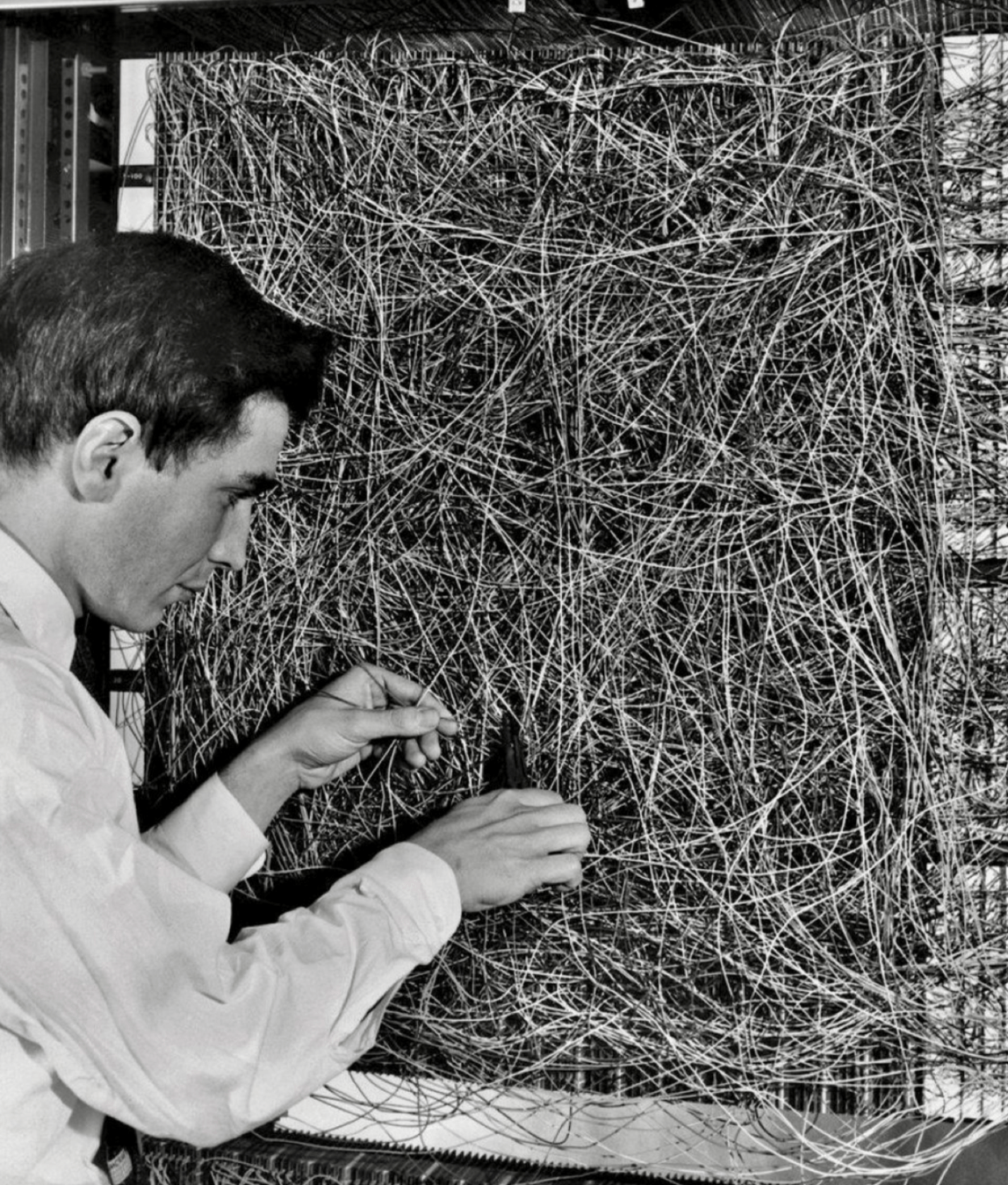
Linear classification helped kick off the first wave of AI enthusiasm.
👆
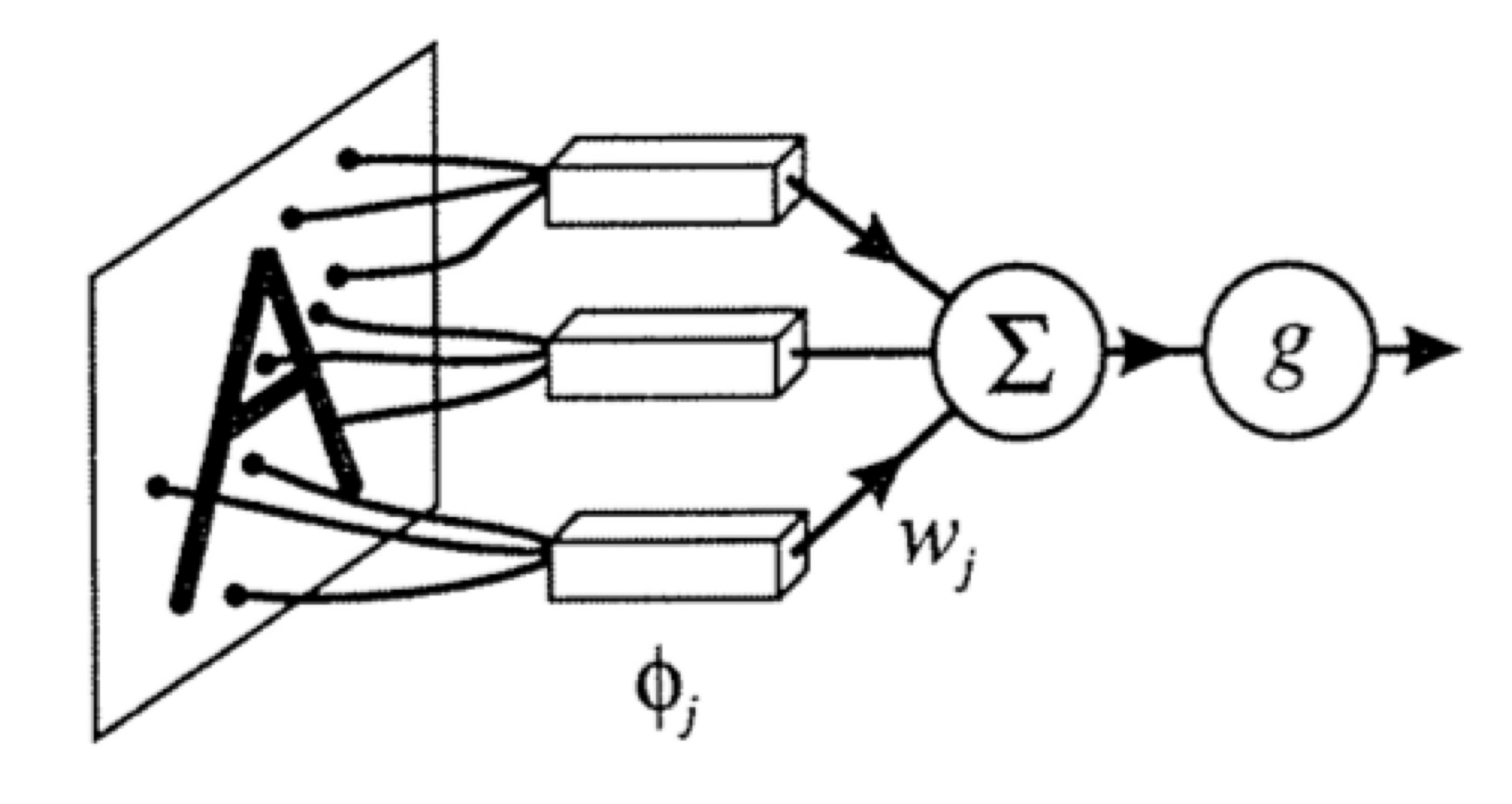

👇
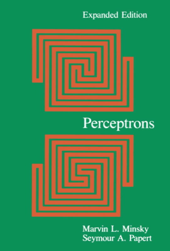
Not linearly separable.
Linear tools cannot solve interesting tasks.
Linear tools cannot, by themselves, solve interesting tasks.
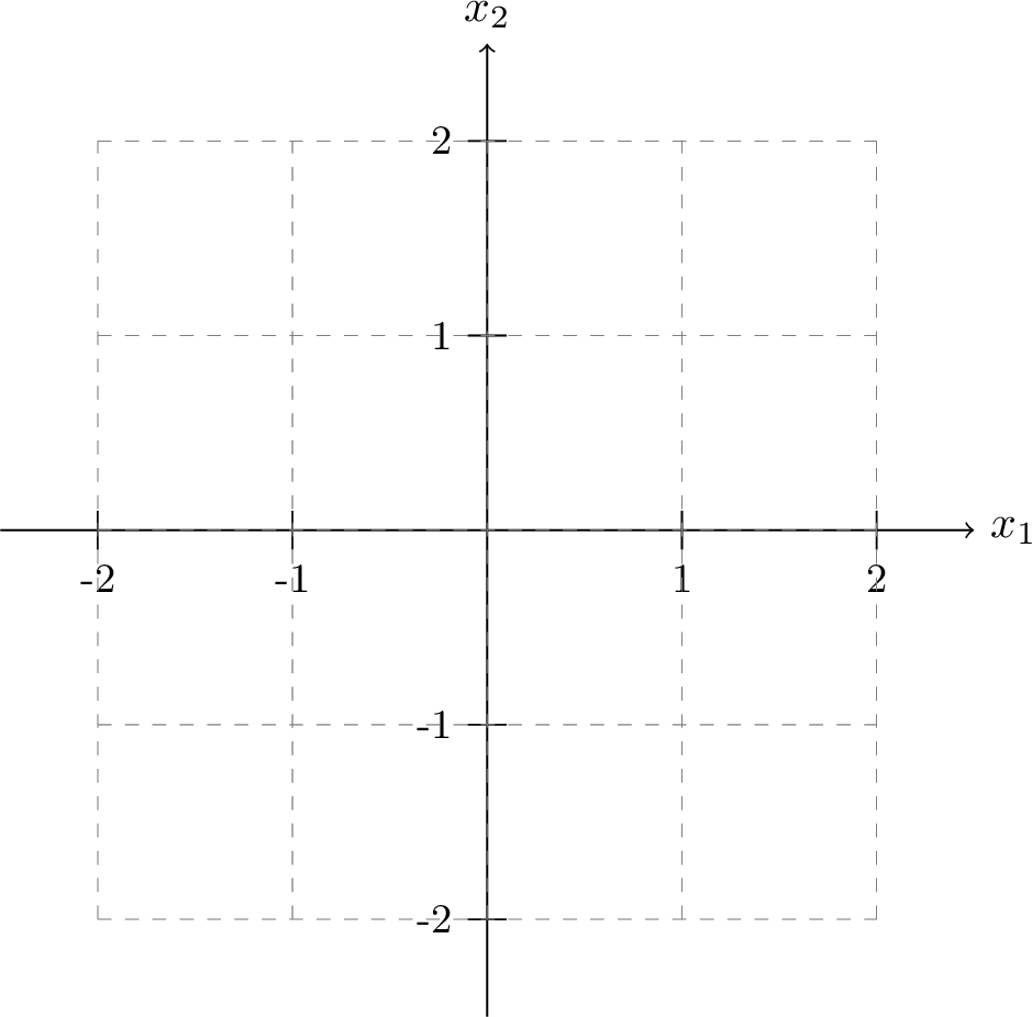
XOR dataset
feature engineering 👉
👈 neural networks
Outline
-
Systematic feature transformations
- Engineered features
- Polynomial features
- Expressive power
- Neural networks
original features \(x \in \mathbb{R}^d \)
new features \(\phi(x) \in \mathbb{R}^{d^{\prime}}\)
nonlinear in \(x\)
linear in \(\phi\)
nonlinear
transformation
\(\phi\)
Linearly separable in \(\phi(x) = x^2\) space
Not linearly separable in \(x\) space
transform via \(\phi(x) = x^2\)
Linearly separable in \(\phi(x) = x^2\) space, e.g. predict positive if \(\phi \geq 3\)
Separable by a nonlinear rule in \(x\) space, e.g. predict positive if \(x^2 \geq 3\)
transform via \(\phi(x) = x^2\)
data and classifier in \(x\) space
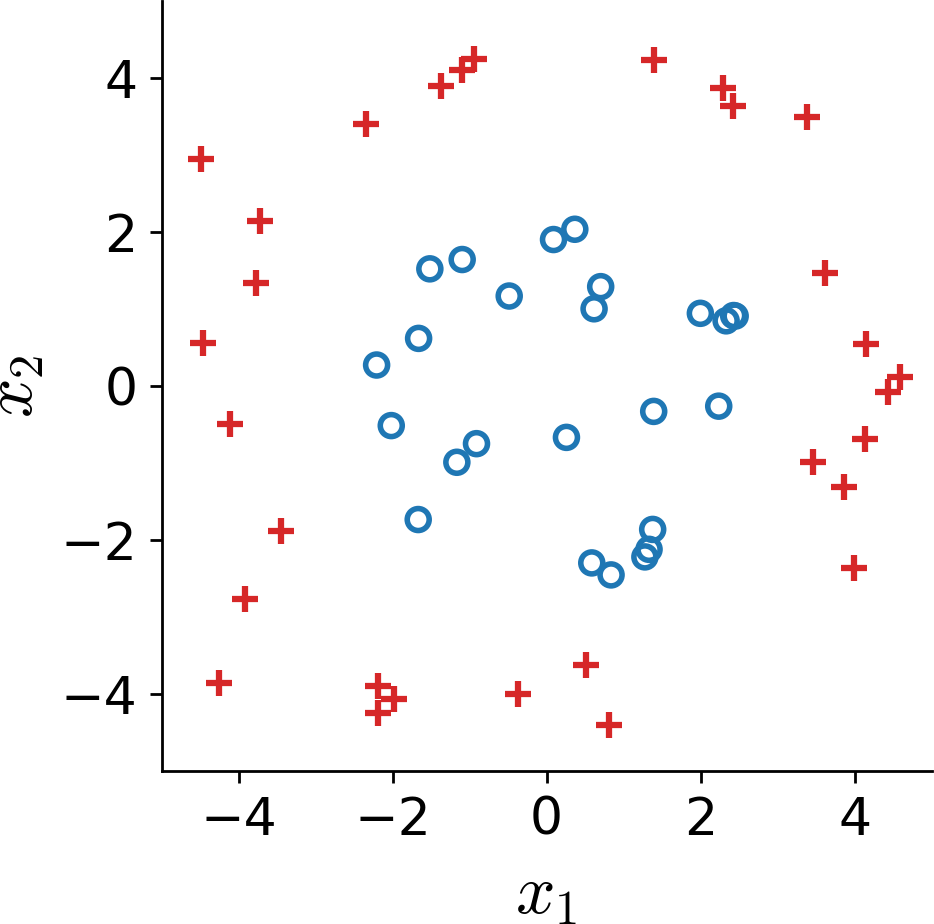
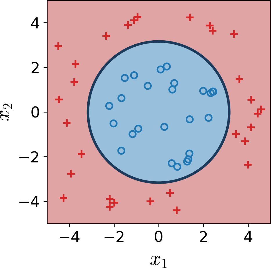
\(x_1^2 + x_2^2 = 10\): nonlinear in \(x\)
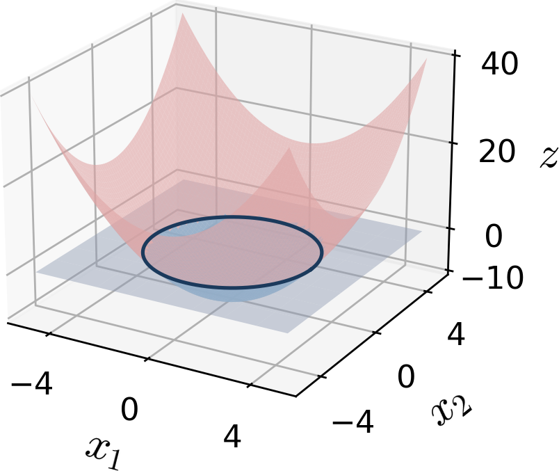
\(z = x_1^2 + x_2^2 - 10\), threshold at \(z\!=\!0\)
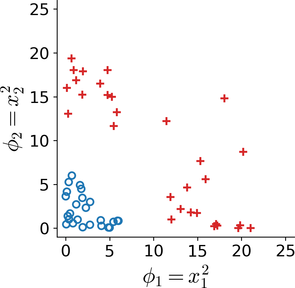
... in \(\phi\) space, where \(\phi(x) = (x_1^2,\, x_2^2)\)
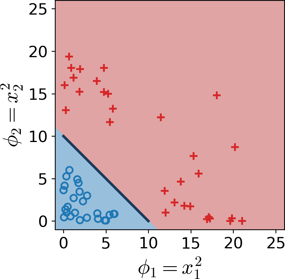
\(\phi_1 + \phi_2 = 10\): linear in \(\phi\)
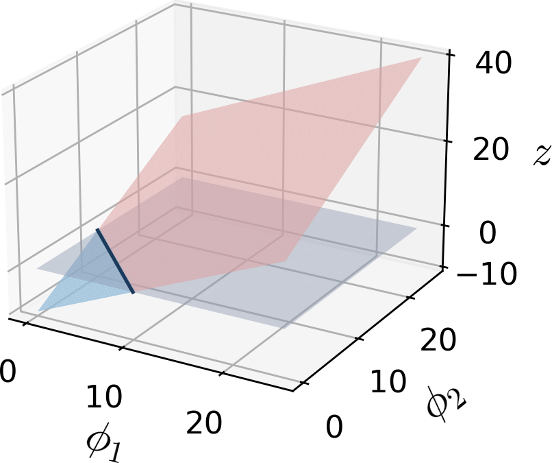
\(z = \phi_1 + \phi_2 - 10\), threshold at \(z\!=\!0\)
decision boundary is linear in \(\phi,\) nonlinear in \(x\)
data in \(x\)-space
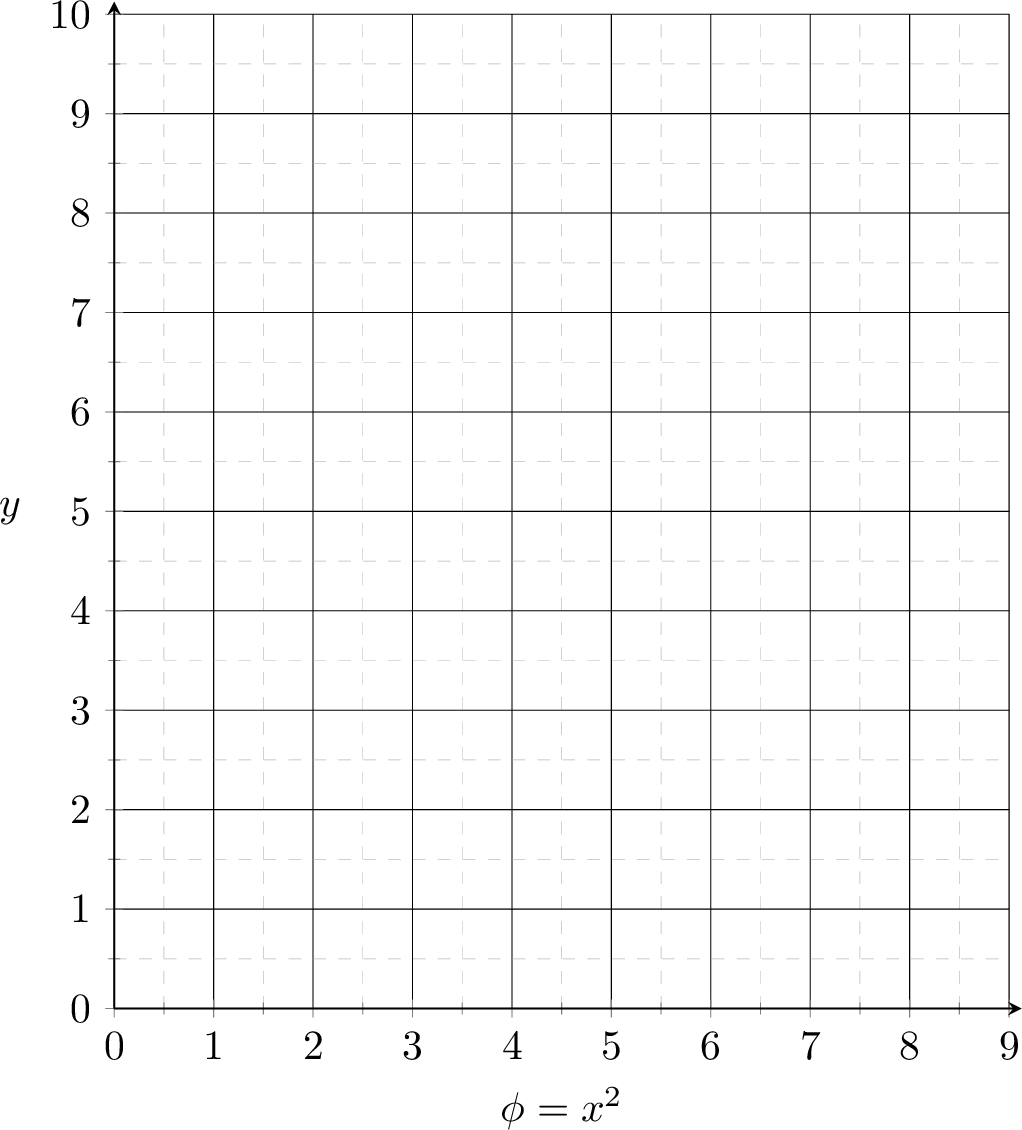
data in \(\phi\)-space
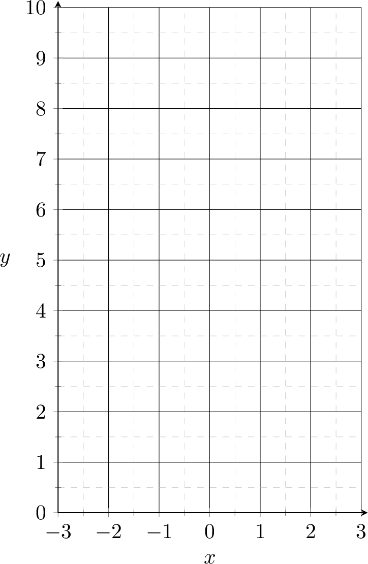
training data
| \(x\) | \(y\) | |
| p1 | -2 | 5 |
| p2 | 1 | 2 |
| p3 | 3 | 10 |
transform via
\(\phi(x)=x^2\)
training data
| \(\phi\) | \(y\) | |
| p1 | 4 | 5 |
| p2 | 1 | 2 |
| p3 | 9 | 10 |
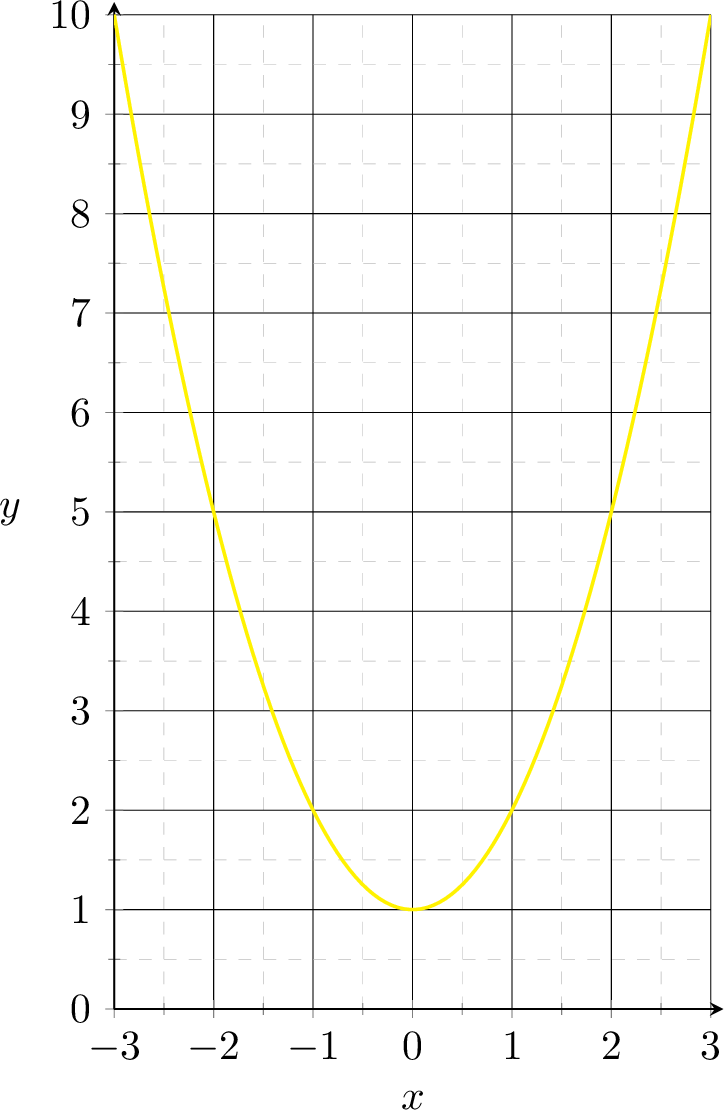
nonlinear regression
\(g = \phi + 1\)
\(g = x^2 + 1\)
systematic construction of polynomial features
| \(d = 1\), features: \(x_1\) | \(d = 2\), features: \(x_1, x_2\) | |
|---|---|---|
| \(k=0\) | \(1\) | \(1\) |
| \(k=1\) | \(1\) \(x_1\) | \(1\) \(x_1,\; x_2\) |
| \(k=2\) | \(1\) \(x_1\) \(x_1^2\) | \(1\) \(x_1,\; x_2\) \(x_1^2,\; x_1 x_2,\; x_2^2\) |
| \(k=3\) | \(1\) \(x_1\) \(x_1^2\) \(x_1^3\) | \(1\) \(x_1,\; x_2\) \(x_1^2,\; x_1 x_2,\; x_2^2\) \(x_1^3,\; x_1^2 x_2,\; x_1 x_2^2,\; x_2^3\) |
| \(\vdots\) | \(\vdots\) | \(\vdots\) |
- The basis holds every monomial of the original features with total degree up to \(k\)
- Fixing \(d\) and \(k\) fixes the basis.
number of features \(d^{\prime} = \dbinom{d+k}{k}\); \(d = 2,\ k = 3\) gives \(10\)
- \(n = 9\) data points, each with feature \(x \in \mathbb{R}\) and label \(y \in \mathbb{R}\)
- data generated from green dashed curve
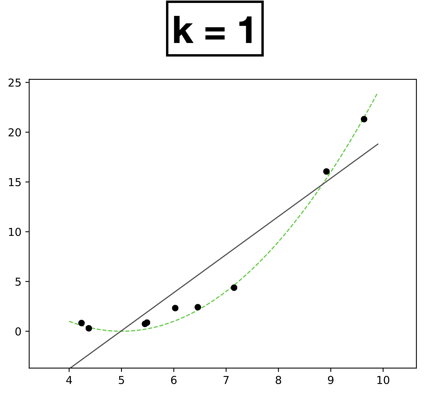
\( h = \textcolor{#4a6fa5}{\theta_0} + \textcolor{#4a6fa5}{\theta_1} \textcolor{#888}{x} \)
Learn 2 parameters — degree-1
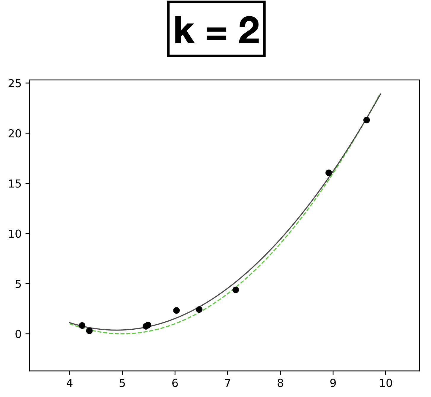
\( h = \textcolor{#4a6fa5}{\theta_0} + \textcolor{#4a6fa5}{\theta_1} \textcolor{#888}{x} + \textcolor{#4a6fa5}{\theta_2} \textcolor{#888}{x^2} \)
Learn 3 parameters — degree-2
Underfitting
Appropriate model
Overfitting
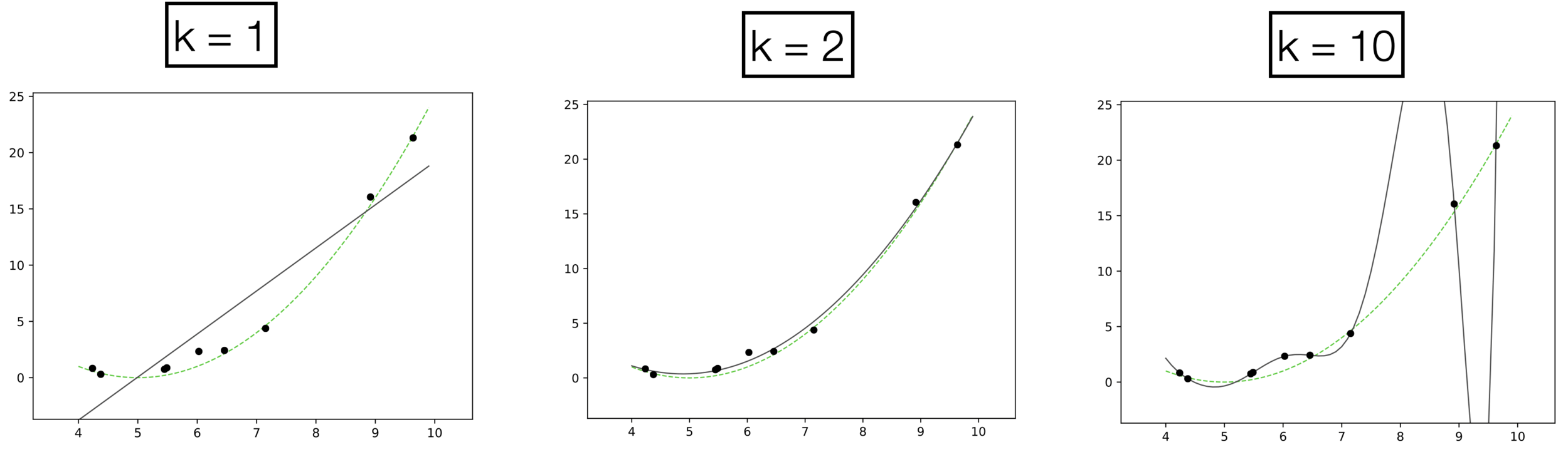
high error on train set
high error on test set
low error on train set
low error on test set
low error on train set
high error on test set
- \(k:\) a hyperparameter that determines the capacity (expressiveness) of the hypothesis class.
- Models with many rich features and free parameters tend to have high capacity but also greater risk of overfitting.
- How to choose \(k?\) Validation/cross-validation.
Previously:
🧠⚙️
hypothesis class
loss function
hyperparameters
\(\left\{\left(x^{(i)}, y^{(i)}\right)\right\}_{i=1}^{n}\)
Linear
Learning Algorithm
\(\left\{\left(\phi(x^{(i)}), y^{(i)}\right)\right\}_{i=1}^{n}\)
Linear
Learning Algorithm
🧠⚙️
hypothesis class
loss function
hyperparameters
today, so far:
🧠⚙️
feature
transformation \(\phi(x)\)
can we automate 👆?
i.e. fold it into the learning algorithm?
\(\left\{\left(x^{(i)}, y^{(i)}\right)\right\}_{i=1}^{n}\)
Nonlinear
Learning Algorithm
🧠⚙️
hypothesis class
loss function
hyperparameters
neural networks:
\(\left\{\left(x^{(i)}, y^{(i)}\right)\right\}_{i=1}^{n}\)
the nonlinearity \(\phi\) is learned, not hand-designed
Something to think about:
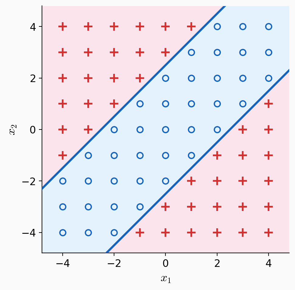
What fixed transformation \(\phi\) can make this decision boundary in \(x\) space?
Outline
- Systematic feature transformations
-
Neural networks
- Terminology
- Design choices
👋 heads-up:
all neural network diagrams focus on a single data point
Outlined the fundamental concepts of neural networks:

expressiveness
efficient learning
- Nonlinear feature transformation
- Composing simple nonlinearities amplifies this effect
- Backpropagation
layered structure
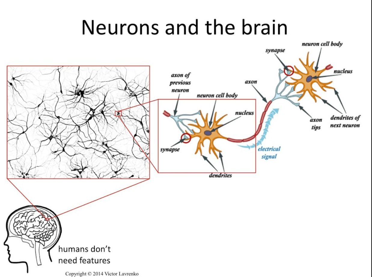
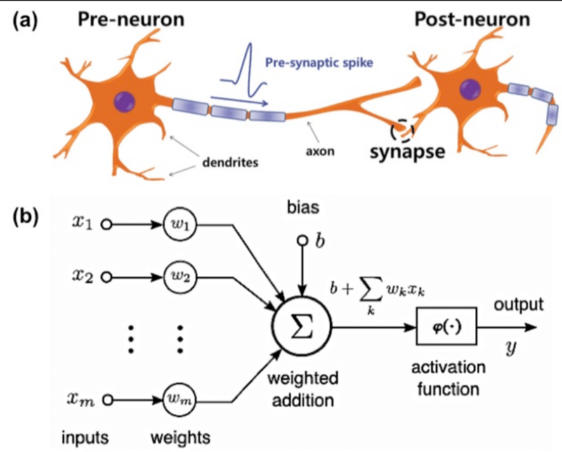
We abstract this into a simple mathematical unit.
importantly, linear in \(\phi\), nonlinear in \(x\)
- Nonlinear feature transformation
transform via
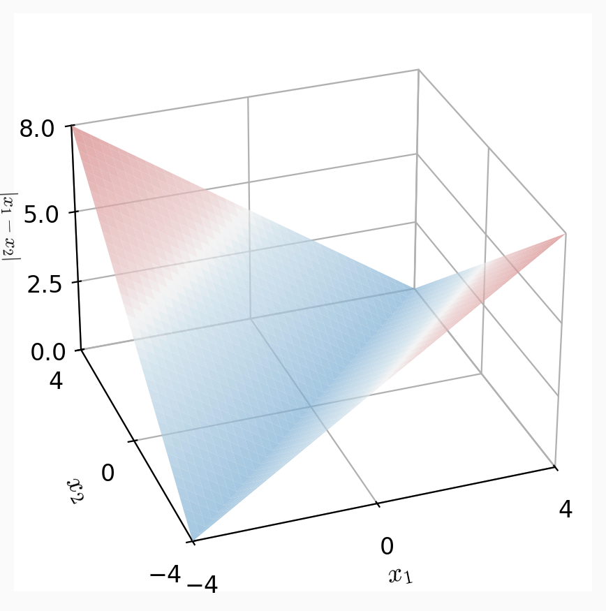
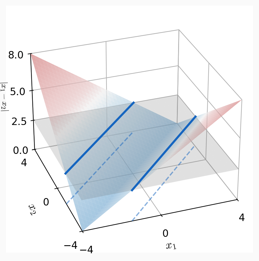
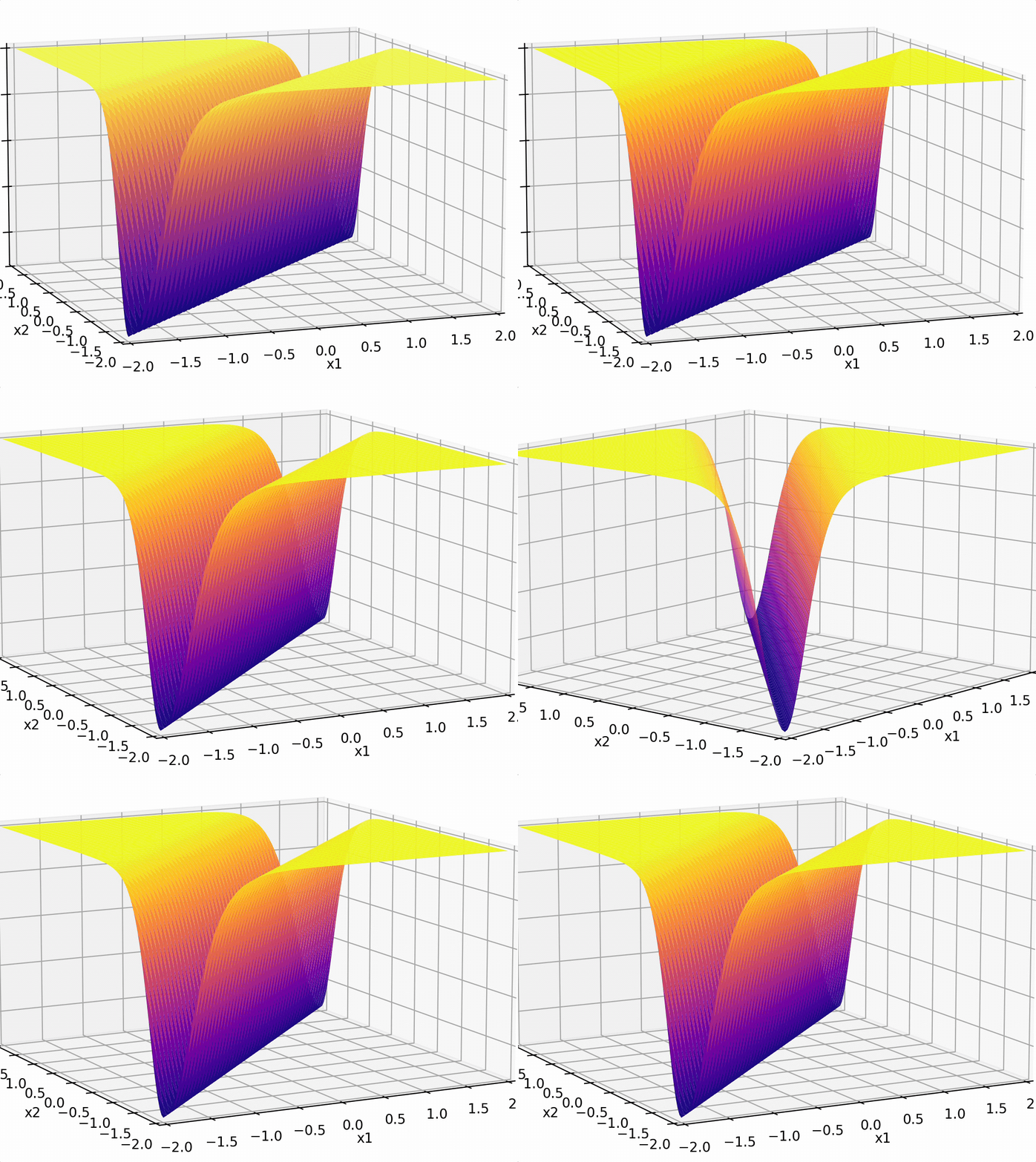
- "Composing" simple transformations
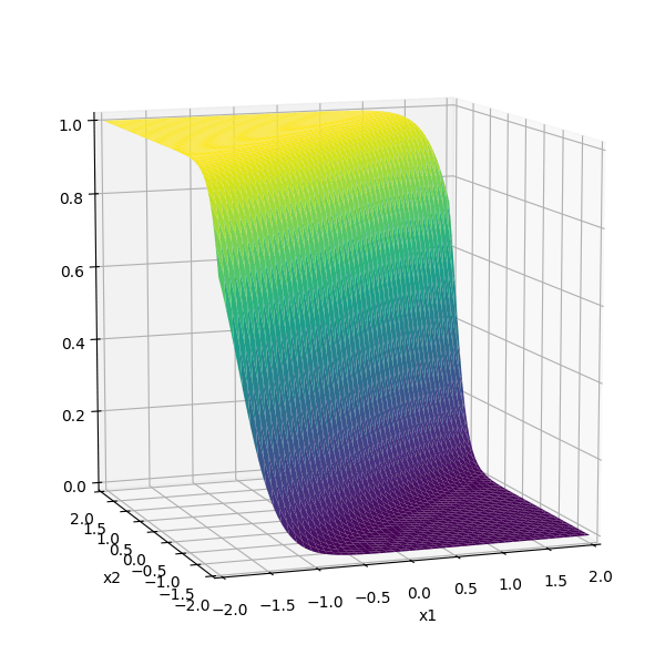
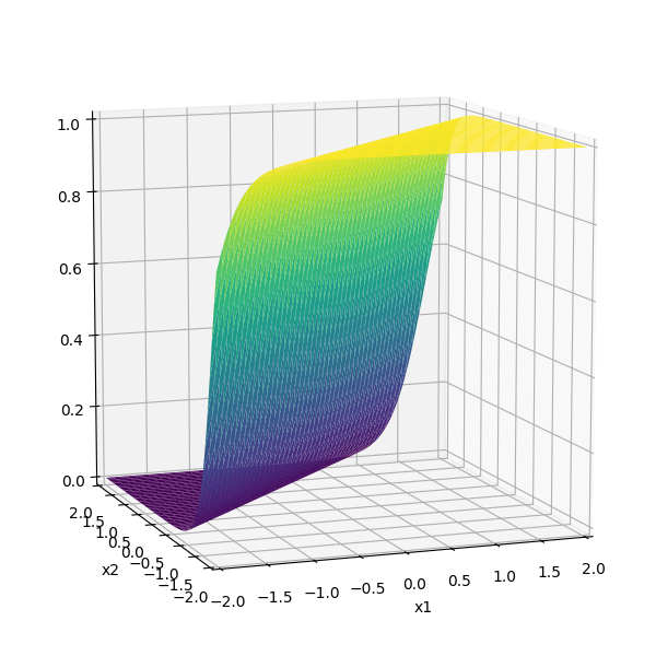
some appropriately weighted sum
- "Composing" simple transformations
A neuron:
\(w\): what the algorithm learns
- \(x\): \(d\)-dimensional input
A neuron:
- \(a\): post-activation output
- \(f\): activation function
- \(w\): weights (i.e. parameters)
- \(z\): pre-activation output
\(f\): what we engineers choose
\(z\): scalar
\(a\): scalar
Choose activation \(f(z)=z\)
learnable parameters (weights)
e.g. linear regressor represented as a computation graph
Choose activation \(f(z)=\sigma(z)\)
learnable parameters (weights)
e.g. linear logistic classifier represented as a computation graph
A layer:
learnable weights
A layer:
- (# of neurons) = layer's output dimension.
- activations apply element-wise, so \(z_1\) doesn't affect \(a_2\) (softmax in the output layer is the common exception).
- all neurons in a layer typically share the same \(f\) (mixed \(f\) is possible but complicates the math).
- layers are typically fully connected: each input \(x_i\) influences every \(a_j\).
layer
linear combo
activations
A (fully-connected, feed-forward) neural network:
layer
input
neuron
learnable weights
Engineers choose:
- activation \(f\) in each layer
- # of layers
- # of neurons in each layer
hidden
output
some appropriately weighted sum
recall this example
\(f =\sigma(\cdot)\)
\(f(\cdot) \) identity function
\(-3(\sigma_1 +\sigma_2)\)
can be represented as:
- Activation \(f\) is chosen as the identity function
- Evaluate the loss \(\mathcal{L} = (g^{(i)}-y^{(i)})^2\)
- Repeat for each data point, average the \(n\) individual losses
e.g. forward pass of a linear regressor
- Activation \(f\) is chosen as the sigmoid function
- Evaluate the loss \(\mathcal{L} = - [y^{(i)} \log g^{(i)}+\left(1-y^{(i)}\right) \log \left(1-g^{(i)}\right)]\)
- Repeat for each data point, average the \(n\) individual losses
e.g. forward pass of a linear logistic classifier
\(\dots\)
Forward pass: evaluate, given the current parameters
- the model outputs \(g^{(i)}\) =
- the loss incurred on the current data \(\mathcal{L}(g^{(i)}, y^{(i)})\)
- the training error \(J = \frac{1}{n} \sum_{i=1}^{n}\mathcal{L}(g^{(i)}, y^{(i)})\)
linear combination
loss function
(nonlinear) activation
Outline
- Systematic feature transformations
-
Neural networks
- Terminology
- Design choices
Choosing the hidden-layer activation \(f\)
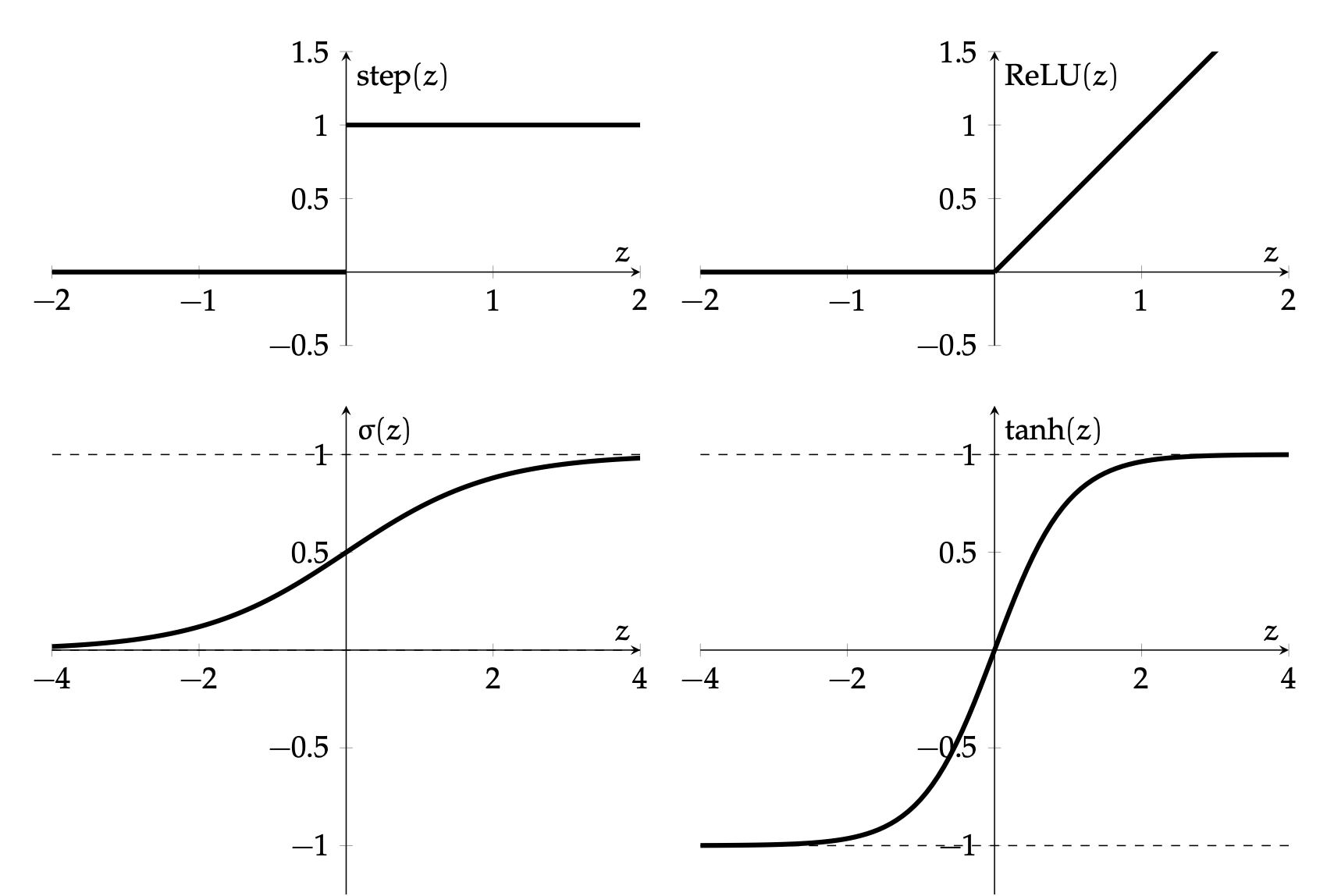
\(\sigma\) used to be the most popular
firing rate of a neuron
elegant gradient \(\sigma^{\prime}(z)=\sigma(z) \cdot(1-\sigma(z))\)
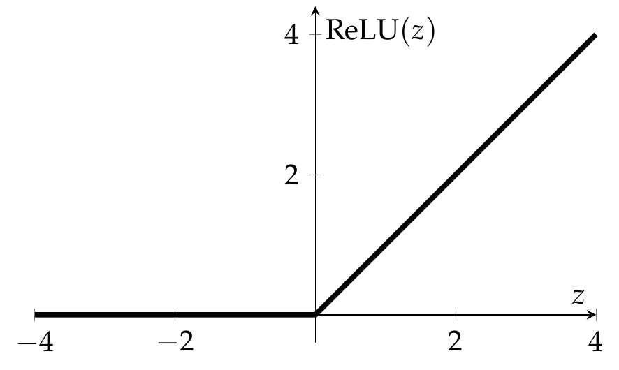
very simple form, and so is its gradient.
nowadays, the default choice:
With learnable \(\textcolor{#38761d}{w}\) and \(\textcolor{#38761d}{w_0}\), which of these can \(\mathrm{ReLU}(\textcolor{#38761d}{w}\,x + \textcolor{#38761d}{w_0})\) draw?
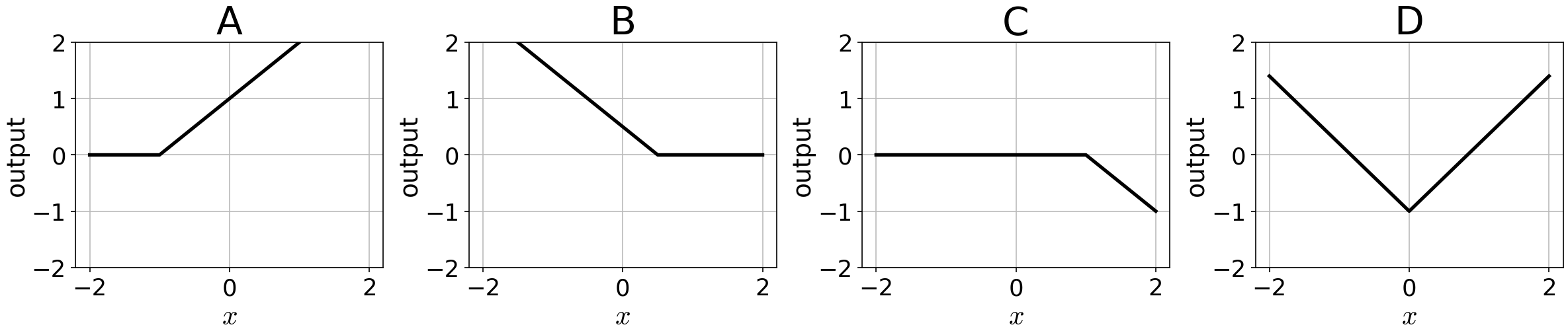
✓
✓
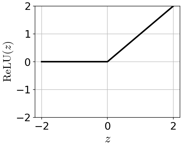
Plotted against \(z,\) \(\mathrm{ReLU}(z)\) looks like this:
compositions of ReLU(s) can be quite expressive, e.g.,
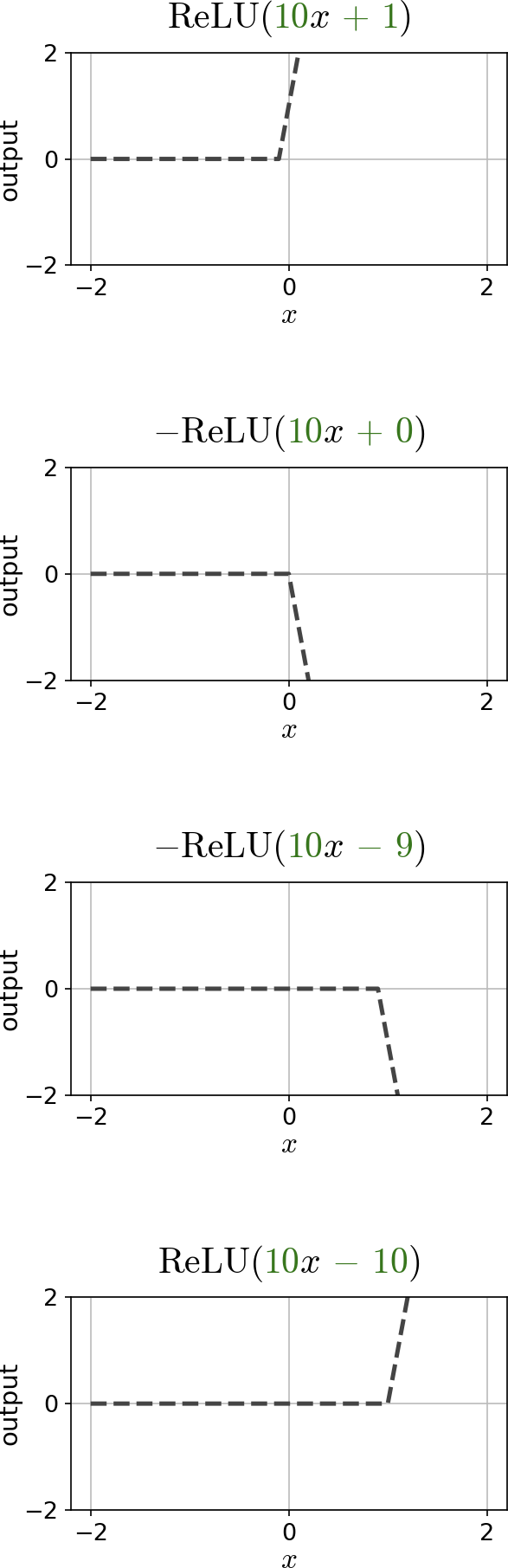
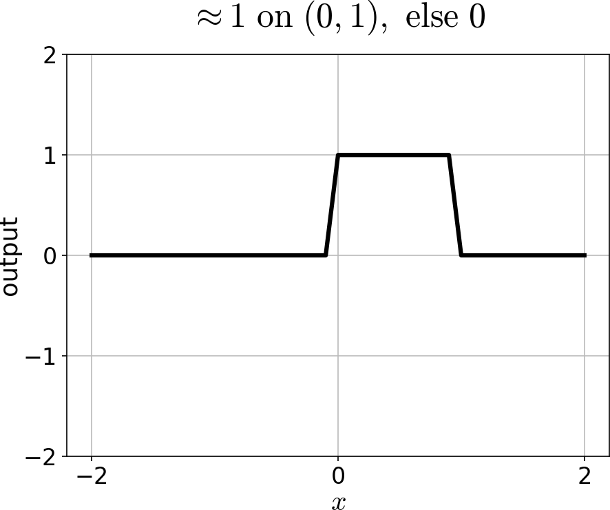
can create bump
with enough of these bumps appropriately scaled and shifted:
asymptotically, can approximate any continuous function arbitrarily well (for regression), therefore can also approximate arbitrary decision boundaries (for classification)
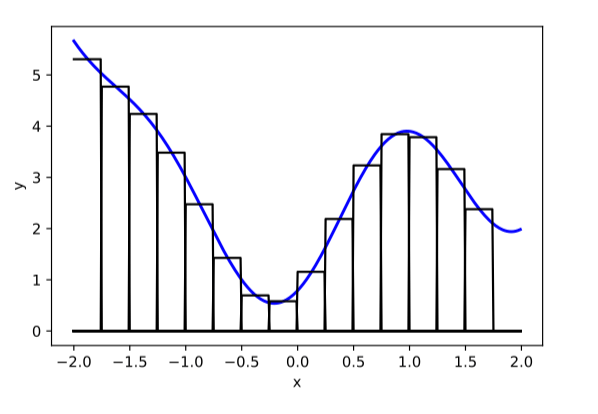
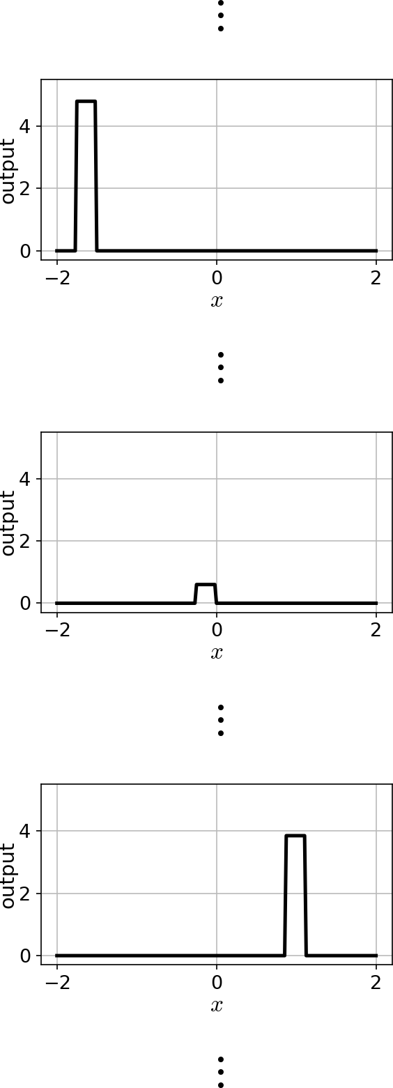
asymptotically: as the number of neurons grows. With enough neurons, even one hidden layer gets within any error of any continuous function on a bounded domain.
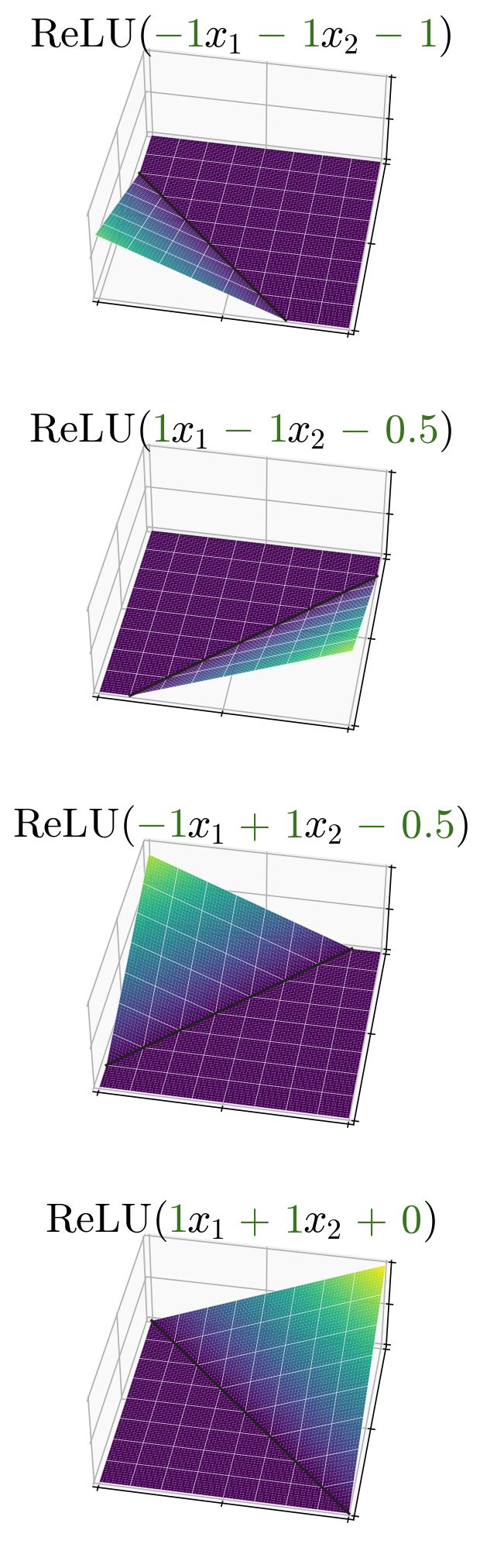
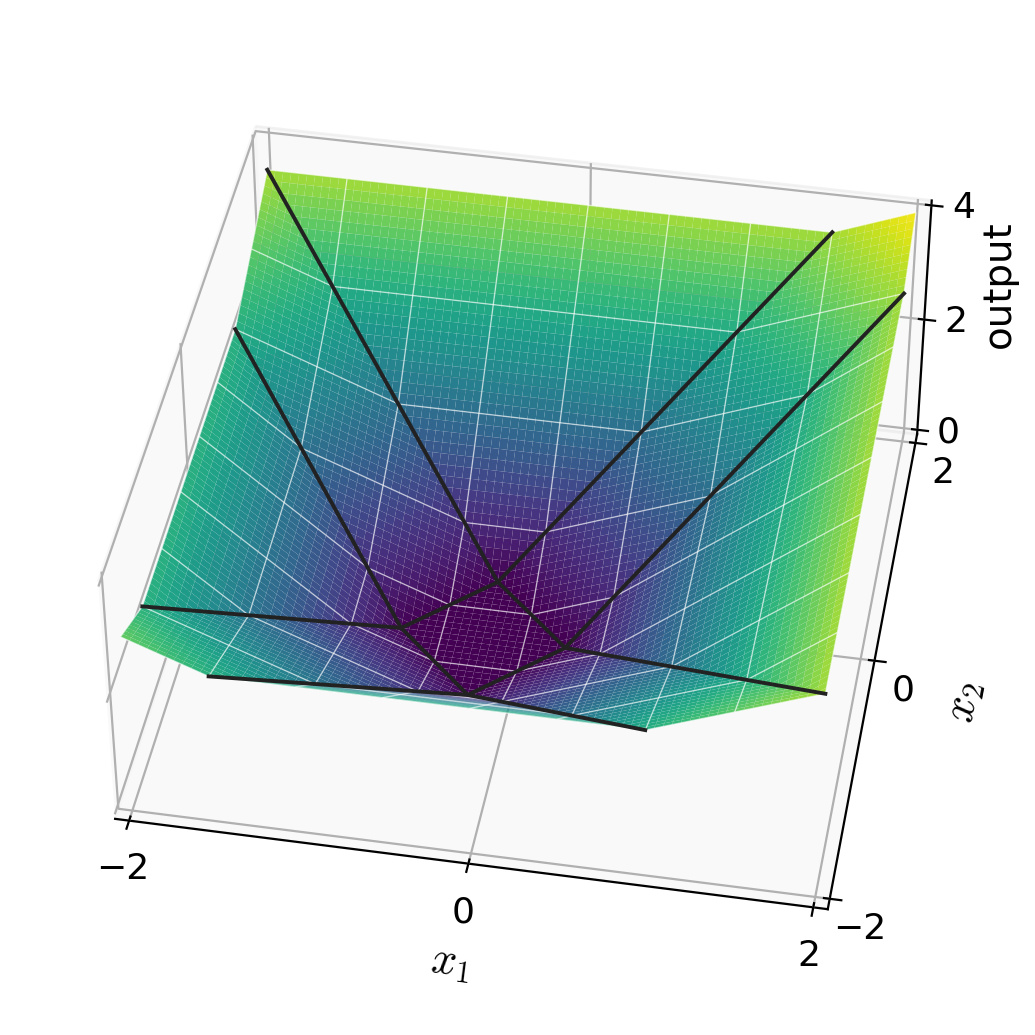
just 4 ReLU neurons already
carve out a non-trivial surface
the same holds for higher dimensions
- Width: # of neurons in layers
- Depth: # of layers
- Typically, increasing either the width or depth (with nonlinear activation) makes the model more expressive, but it also increases the risk of overfitting.
For neural networks, though, how size relates to overfitting is still open research; see the double-descent curve and scaling laws.
(The demo doesn't show in the PDF; the link below works.)
output layer design choices
- # neurons, activation, and loss depend on the high-level goal.
- Typically straightforward.
- Multi-class setup: to predict exactly one of \(K\) classes, the output layer has \(K\) neurons, softmax activation, and cross-entropy loss
- For other multi-class settings, see hw/lab.
e.g., say \(K=5\) classes
input \(x\)
hidden layer(s)
output layer
Summary
Linear models are convenient but lack expressiveness for most real-world tasks.
A fixed nonlinear feature transformation lets us use linear methods on complex problems, but designing features by hand gets tedious.
Neural networks automate feature learning: layers alternate parameterized linear maps with nonlinear activations (typically ReLU).
For classification outputs, we apply sigmoid (binary) or softmax (multi-class).
Next time: How do we train neural networks? (gradient descent + backpropagation)
feature transformations feature transformationpolynomial featuresfeature engineering
neural networks neuronactivation functionlayerhidden layerforward pass
design choices ReLUwidthdepth