

Lecture 9: Transformers
Intro to Machine Learning

[video edited from 3b1b]
Recap: Word embedding
this enables "soft" dictionary look-up:
dict_en2fr = {
  "apple" : "pomme",
  "banana": "banane",
  "lemon" : "citron"}
Good word-embeddings space is equipped with semantically meaningful vector arithmetic
Key
Value
apple
pomme
\(:\)
banane
banana
\(:\)
citron
lemon
\(:\)
Python would complain. 🤯
orange
Query
Output
???
query = "orange"
output = dict_en2fr[query]
But we can probably see the rationale behind something like this:
Query
Key
Value
Output
orange
apple
\(:\)
pomme
banana
\(:\)
banane
lemon
\(:\)
citron
dict_en2fr = {
  "apple" : "pomme",
  "banana": "banane",
  "lemon" : "citron"}

query = "orange"
output = dict_en2fr[query]
0.1
pomme
0.1
banane
0.8
citron
+
+
0.1
pomme
0.1
banane
0.8
citron
+
+
Query
Key
Value
Output
orange
apple
\(:\)
pomme
0.1
pomme
0.1
banane
0.8
citron
banana
\(:\)
banane
lemon
\(:\)
citron
+
+
orange
orange
pomme
banane
citron
+
+
0.8
0.1
0.1
pomme
banane
citron
+
+
- output mixed values:
- compare query and key (dot-product similarity) for merging percentages:
apple
banana
lemon
orange
orange
orange
softmax
0.1
0.1
0.8
The attention mechanism in transformers mimics this:
We picked these percentages by hand; let's see how a transformer comes up with them.
Outline
- Intuition and overview
- Attention mechanism
- Multi-head attention
- Attention beyond language
- Intuition and overview
- Attention mechanism
- Multi-head attention
- Attention beyond language
Large Language Models (LLMs) are trained in this self-supervised way:
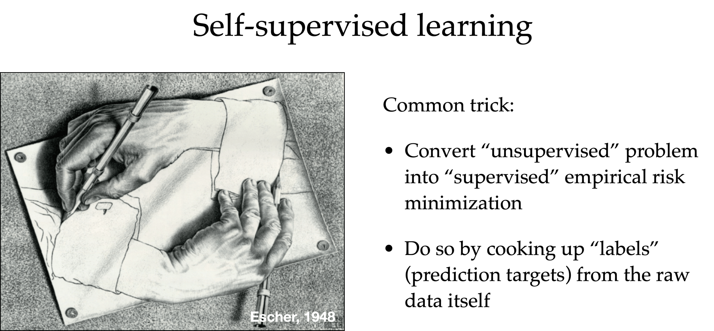
- Scrape the internet for plain texts.
- Cook up “labels” from these texts.
- Use the unhidden part to predict the hidden label.
"To date, the cleverest thinker of all time was Isaac."
feature
label
To date, the
cleverest
To date, the cleverest
thinker
To date, the cleverest thinker
was
To date, the cleverest thinker of all time was
Isaac
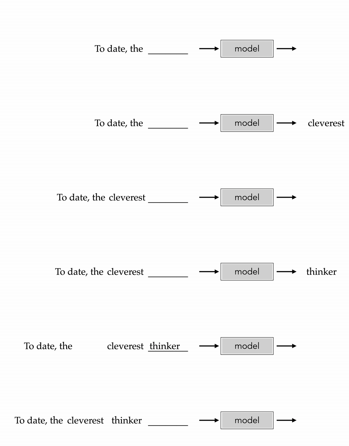
auto-regressive prediction
[video edited from 3b1b]
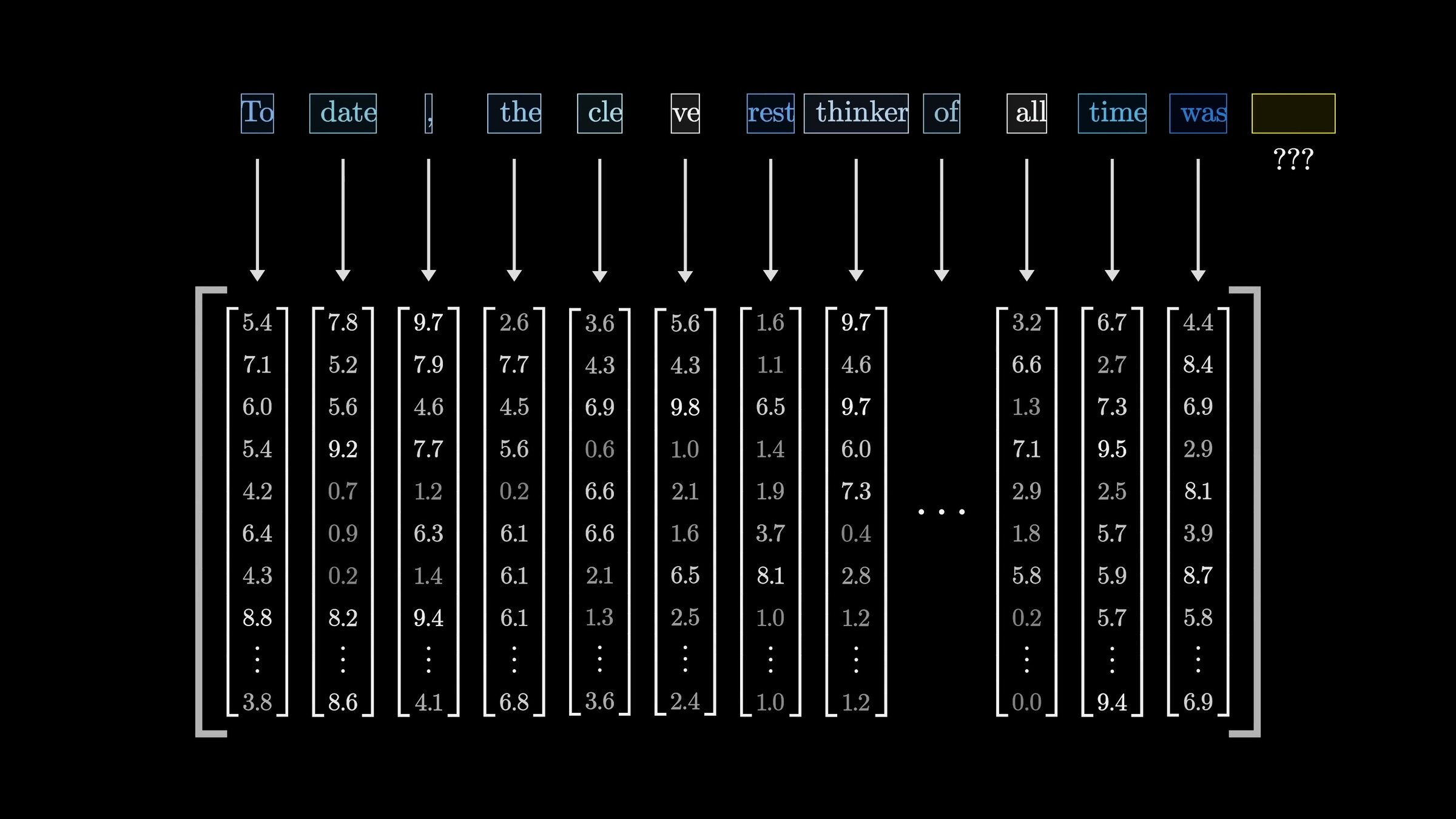
\(n\)
\(d\)
input embedding
[video edited from 3b1b]
Minimizing cross-entropy loss drives the weights to assign higher probability to the correct next token
word embedding to a softmax distribution over the vocabulary
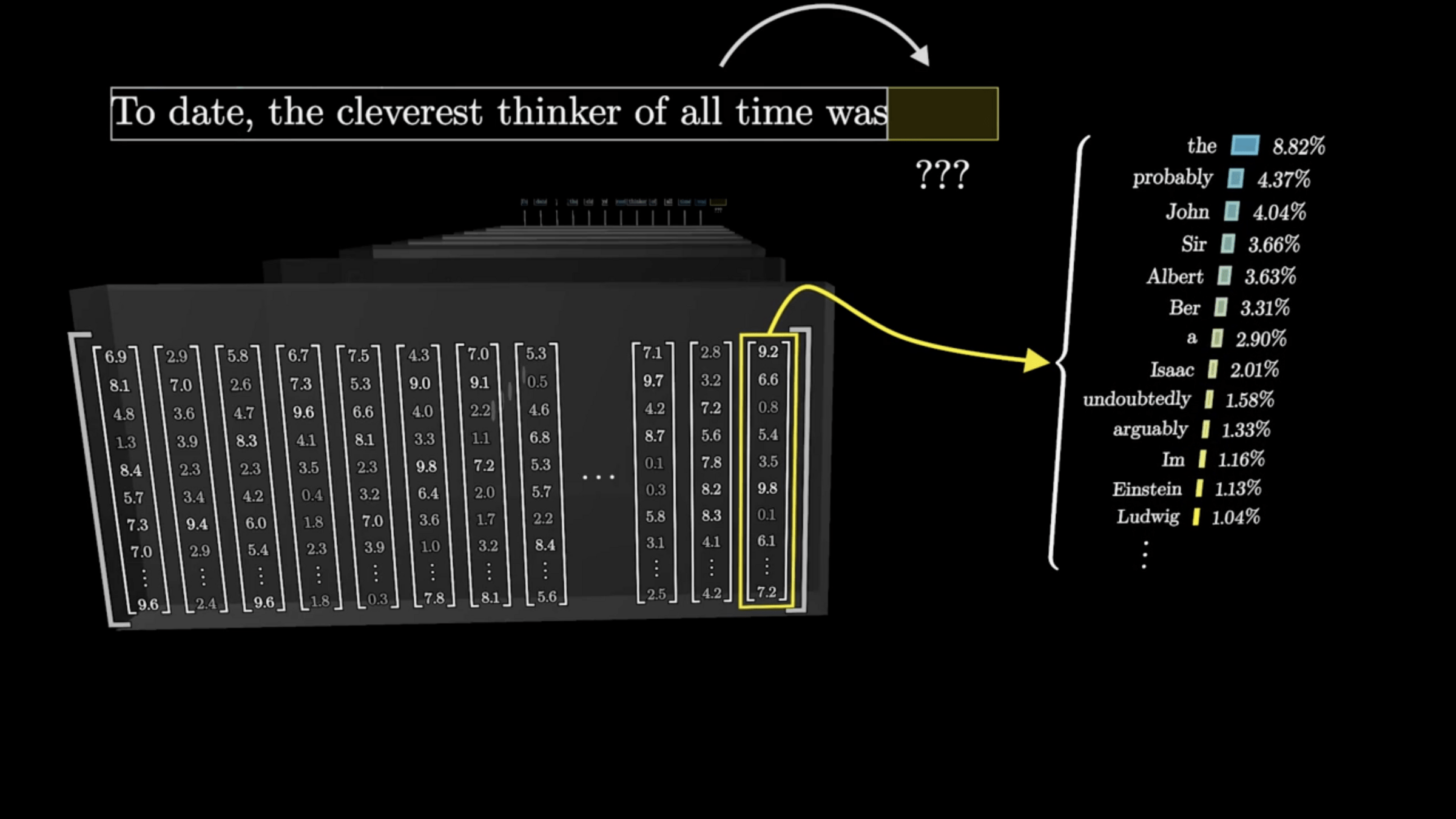
Transformer
"To date, the cleverest [thinker] of all time was Isaac.
push for Prob("date") to be high
push for Prob("the") to be high
push for Prob("cleverest") to be high
push for Prob("thinker") to be high
distribution over the vocabulary
\(\dots\)
\(\dots\)
\(\dots\)
\(\dots\)
To
date
the
cleverest
input embedding
\(\dots\)
\(\dots\)
\(\dots\)
transformer block
transformer block
transformer block
\(L\) blocks
\(\dots\)
\(\dots\)
output embedding
To
date
the
cleverest
\(\dots\)
transformer block
transformer block
transformer block
A sequence of \(n\) tokens, each token in \(\mathbb{R}^{d}\)
\(\dots\)
\(\dots\)
\(\dots\)
\(\dots\)
output embedding
input embedding
input embedding
To
date
the
cleverest
[video edited from 3b1b]
input embedding
\(\dots\)
transformer block
output embedding
\(\dots\)
\(\dots\)
\(\dots\)
\(\dots\)
transformer block
transformer block
each of the \(n\) tokens transformed, block by block
within a shared \(d\)-dimensional word-embedding space.
To
date
the
cleverest
attention layer
MLP
\(\dots\)
\(\dots\)
\(\dots\)
\(\dots\)
neuron weights
input embedding
transformer block
output embedding
To
date
the
cleverest
attention layer
attention output projection
\((qkv)\) projection
attention mechanism
word space
\(\mathbb{R}^{d}\)
word space
\(\mathbb{R}^{d}\)
working space
\(\mathbb{R}^{d_k}\)
working space
\(\mathbb{R}^{d_k}\)
1.
2.
e.g., for GPT-2, \(d = 768\), \(d_k = 64\), both hyperparameters
working space \(d_k \ll\) word space \(d\)
1. (query, key, value) projection — why do we need anything beyond the word space?
To
\(\leftarrow\) word space \(\mathbb{R}^{d}\)
\(\leftarrow\) working space \(\mathbb{R}^{d_k}\)
\(x\) has to play three roles:
- \(q\): what it looks for (\(W_q\) learns how to ask)
- \(k\): what it offers (\(W_k\) learns how to listen)
- \(v\): what it hands over (\(W_v\) learns how to speak)
\(\leftarrow W_q, W_k, W_v \in \mathbb{R}^{d \times d_k}\)
1. (query, key, value) projection — why do we need anything beyond the word space?
To
date
the
cleverest
\(x\) has to play three roles:
- \(q\): what it looks for (\(W_q\) learns how to ask)
- \(k\): what it offers (\(W_k\) learns how to listen)
- \(v\): what it hands over (\(W_v\) learns how to speak)
same \(W_q, W_k, W_v\) for every token: weight sharing, all in parallel
- Attention mechanism turns the projected \((q,k,v)\) into \(z\)
- Each \(z\) is context-aware: a mixture of everyone's values, weighted by relevance
2. Attention mechanism
attention mechanism
To
date
the
cleverest
Outline
- Intuition and overview
- Attention mechanism
- Multi-head attention
- Attention beyond language
attention mechanism
To
date
the
cleverest
softmax
To
date
the
cleverest
dot-product magnitude tend to grow with \(d_k\); without the scaling they saturate the softmax, and gradients get tiny
e.g., softmax\((1, 2, 3, 4) \approx (0.03, 0.09, 0.24, 0.64)\), but softmax\((10, 20, 30, 40) \approx (0, 0, 0, 1)\)
softmax
To
date
the
cleverest
softmax'd attention scores: mixing percentages that sum to 1 (100%)
\(a_{12}\): how much \(x_1\) attends to \(x_2\) when updating \(x_1\)'s representation
softmax
To
date
the
cleverest
\(\in \mathbb{R}^{d_k}\)
attention mechanism
To
date
the
cleverest
softmax
To
date
the
cleverest
softmax
To
date
the
cleverest
attention mechanism
To
date
the
cleverest
softmax
parallel and structurally identical processing
can calculate \(z_4\) without \(z_3\)
To
date
the
cleverest
softmax
To
date
the
cleverest
attention mechanism
a head maps the sequence of \(x\)'s to a sequence of context-aware \(z\)'s, in two steps:
1. learned (query, key, value) projection
2. attention mechanism
Attention head
1. (query, key, value) projection
stack each token \(x_i\) as a row
To
date
the
cleverest
2a. dot-product similarity
compare \(q_i\) and \(k_j\): entry \((i, j)\) is \(q_i^Tk_j\)
2a. dot-product similarity
assemble all \(n \times n\) similarities: row \(i\) is query \(i\)
each row sums up to 1
softmax
softmax
softmax
softmax
softmax
row
\(A\)
2b. attention matrix
2c. attention-weighted values \(Z\)
softmax
row
attention mechanism
attention scores depend on the (query, key) only
recap
attention mechanism
\(z_3\) is meant to help predict \(x_4\)
but \(z_3\) already uses \(v_4\): it peeks at the answer
recap
softmax
To
date
the
cleverest
masking
mask the future:
\(q_3^Tk_4 \to -\infty\), so \(a_{34} = 0\)
masking: no token can peek ahead
dot-product similarity scores
causal mask \(M\)
masked scores
causal attention
matrix \(A\)
\(Z = AV\), same as before
each \(z_i\) now mixes only \(v_1, \dots, v_i\)
Outline
- Intuition and overview
- Attention mechanism
- Multi-head attention
- Attention beyond language
attention mechanism
One attention head
attention mechanism
Two attention heads
head 2 learns its own \(\textcolor{#6aa84f}{W_q^2, W_k^2, W_v^2}\), so it can attend to different things
attention mechanism
H attention heads
In particular, each head:
- learns its own \(W_q, W_k, W_v\)
- creates its own sequence of \(q, k, v\)
- computes its own sequence of \(z\)
Parallel, and structurally identical processing across all heads and tokens.
Multi-head Attention
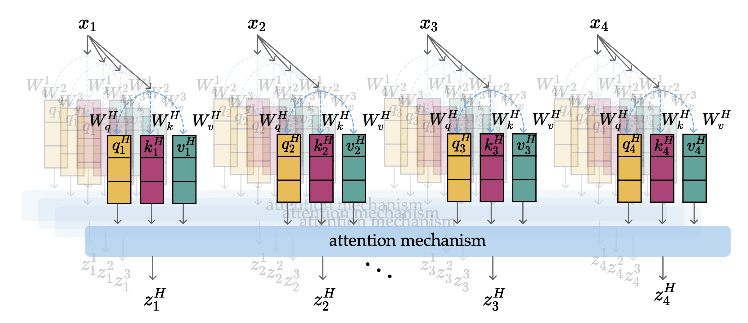
index along heads
index along sequence
concatenate each token's \(H\) head outputs \(z_i^h \in \mathbb{R}^{d_k}\): \(z_i^{\text{concat}} \in \mathbb{R}^{H d_k}\)
attention mechanism
attention mechanism
attention mechanism
attention mechanism
attention mechanism
attention mechanism
attention mechanism
attention mechanism
attention output projection
\(\in \mathbb{R}^{d}\)
\(\textcolor{#6aa84f}{W_o}\): the learned mixer, blending what the heads found back into the word space \(\mathbb{R}^d\)
typically \(H \cdot d_k = d\)
(e.g. GPT-2: 12 heads, \(12 \times 64 = 768,\) all hyperparameters)
attention mechanism
attention mechanism
attention mechanism
attention mechanism
attention output projection
all in word space \(\mathbb{R}^{d}\)
multi-head attention
attention layer
attention output projection
\((qkv)\) projection, \(H\) heads
attention mechanism, \(H\) heads
word space
\(\mathbb{R}^{d}\)
word space
\(\mathbb{R}^{d}\)
each head's working space
\(\mathbb{R}^{d_k}\)
concat heads
\(z_i^{\text{concat}} \in \mathbb{R}^{Hd_k}\)
1.
2.
multi-head attention layer, zoomed out
single-head version: slide 17
zoomed out further, inside a transformer block: slide 16
Shape Example:
\(W\)s are the learned weights
\(n\)
num tokens
5
\(d\)
word-space dim
6
\(X\)
input
\(n \times d\)
\(5 \times 6\)
\(W_q^h\)
query proj
\(d \times d_k\)
\(6 \times 3\)
\(W_k^h\)
key proj
\(d \times d_k\)
\(6 \times 3\)
\(W_v^h\)
value proj
\(d \times d_k\)
\(6 \times 3\)
\(Q^h\)
query
\(n \times d_k\)
\(5 \times 3\)
\(K^h\)
key
\(n \times d_k\)
\(5 \times 3\)
\(V^h\)
value
\(n \times d_k\)
\(5 \times 3\)
\(A^h\)
attn matrix
\(n \times n\)
\(5 \times 5\)
\(Z^h\)
attn head out
\(n \times d_k\)
\(5 \times 3\)
for a single
attention head
\(H\)
num heads
2
\(Z^{\text{concat}}\)
concatenated heads
\(n \times Hd_k\)
\(5 \times 6\)
\(W_o\)
output proj
\(Hd_k \times d\)
\(6 \times 6\)
\(O\)
attn layer out
\(n \times d\)
\(5 \times 6\)
\(d_k\)
working-space dim
3
Practical techniques
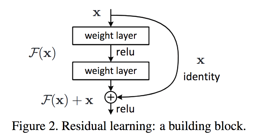
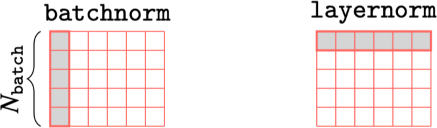

Layer normalization
Residual connection
Positional encoding
Explore interactively: Transformer Explainer
attention alone ignores token order; positional encoding adds each token's position into \(x_i\)
we'll work through these in the lab
Outline
- Intuition and overview
- Attention mechanism
- Multi-head attention
- Attention beyond language
image credit: Nicholas Pfaff

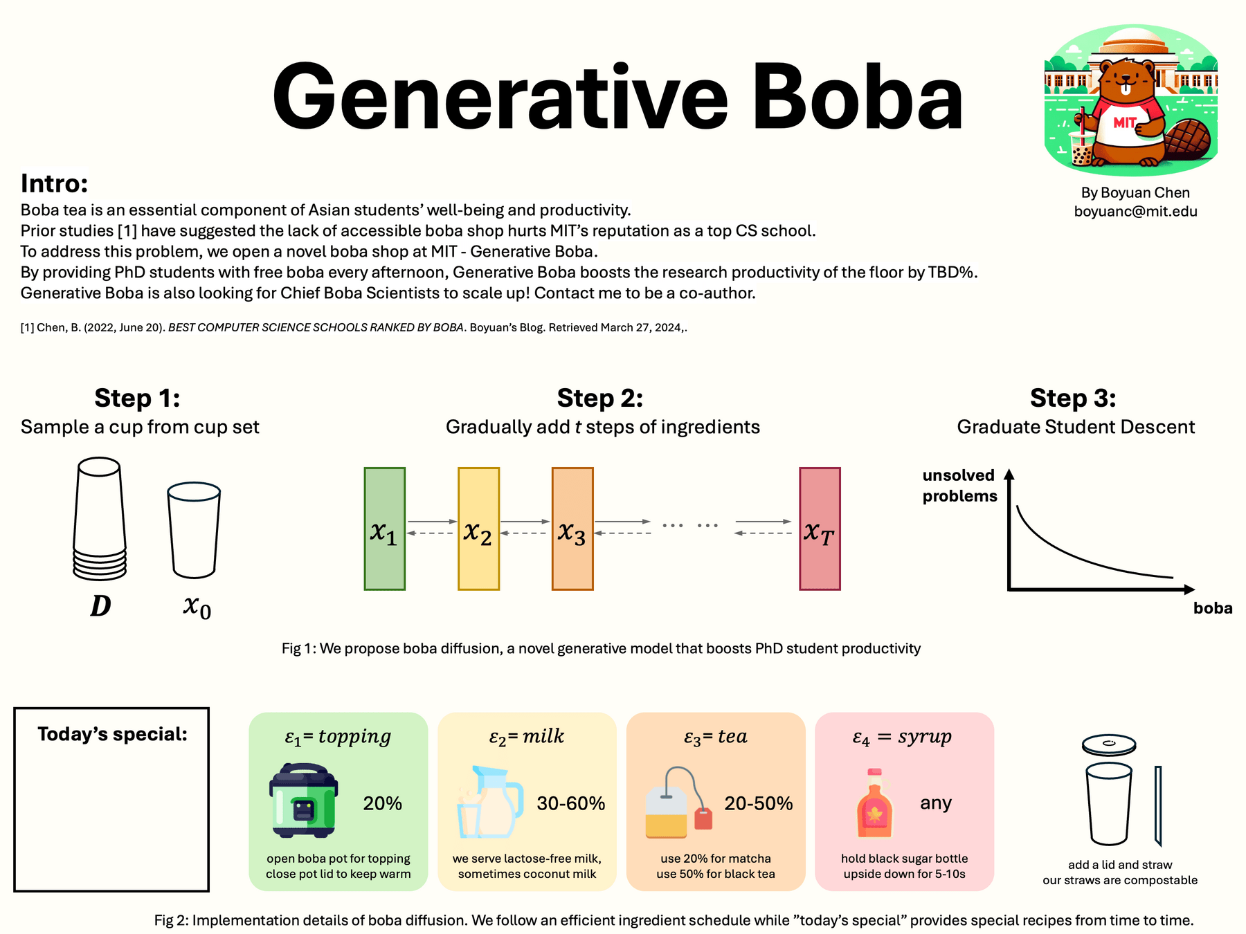
Generative Boba by Boyuan Chen (now at OpenAI)
😉
😉
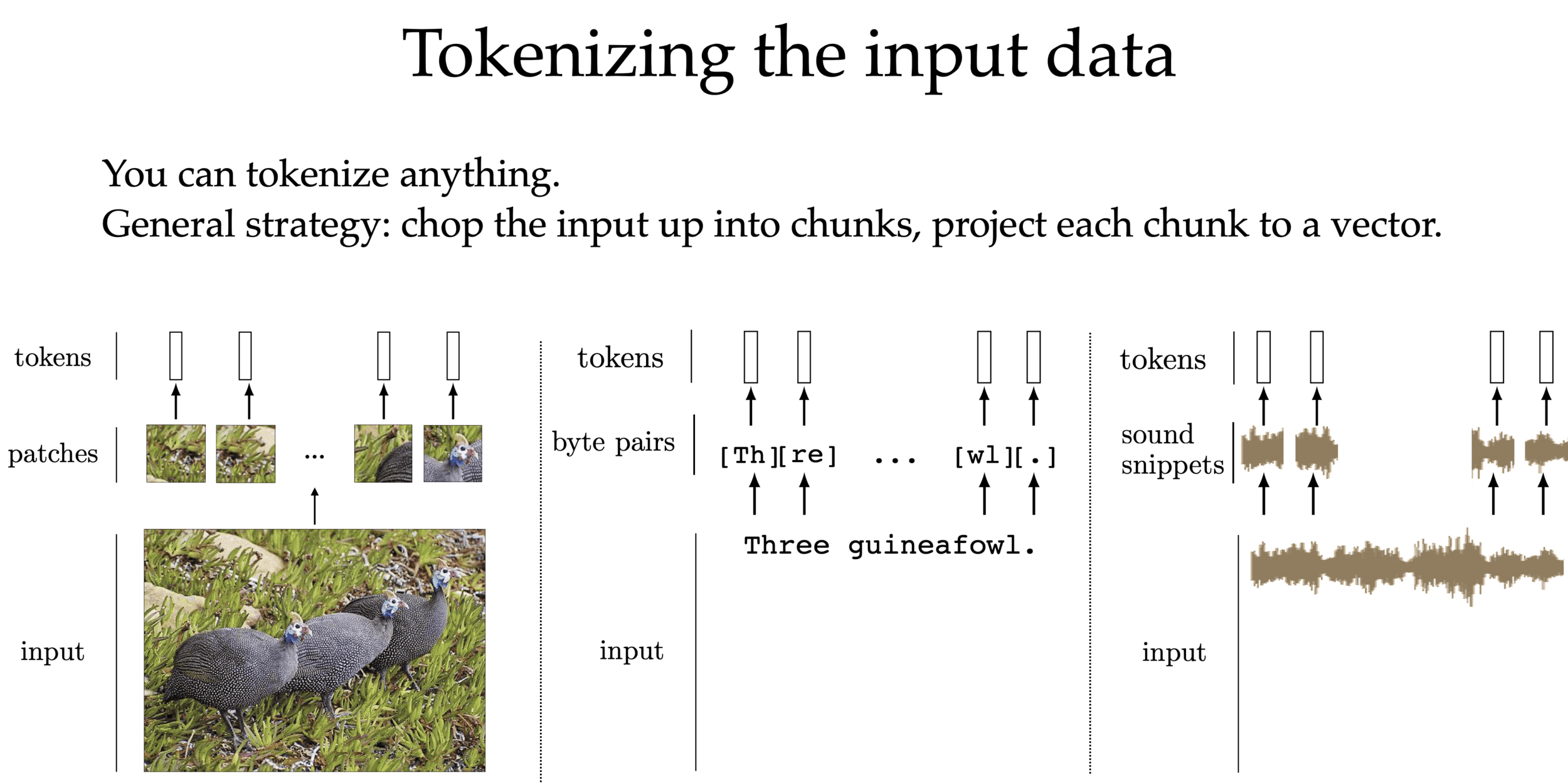
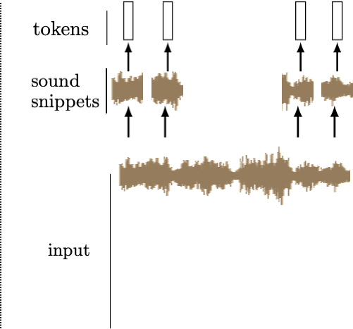
We can tokenize anything.
General strategy: chop the input up into chunks, project each chunk to an embedding
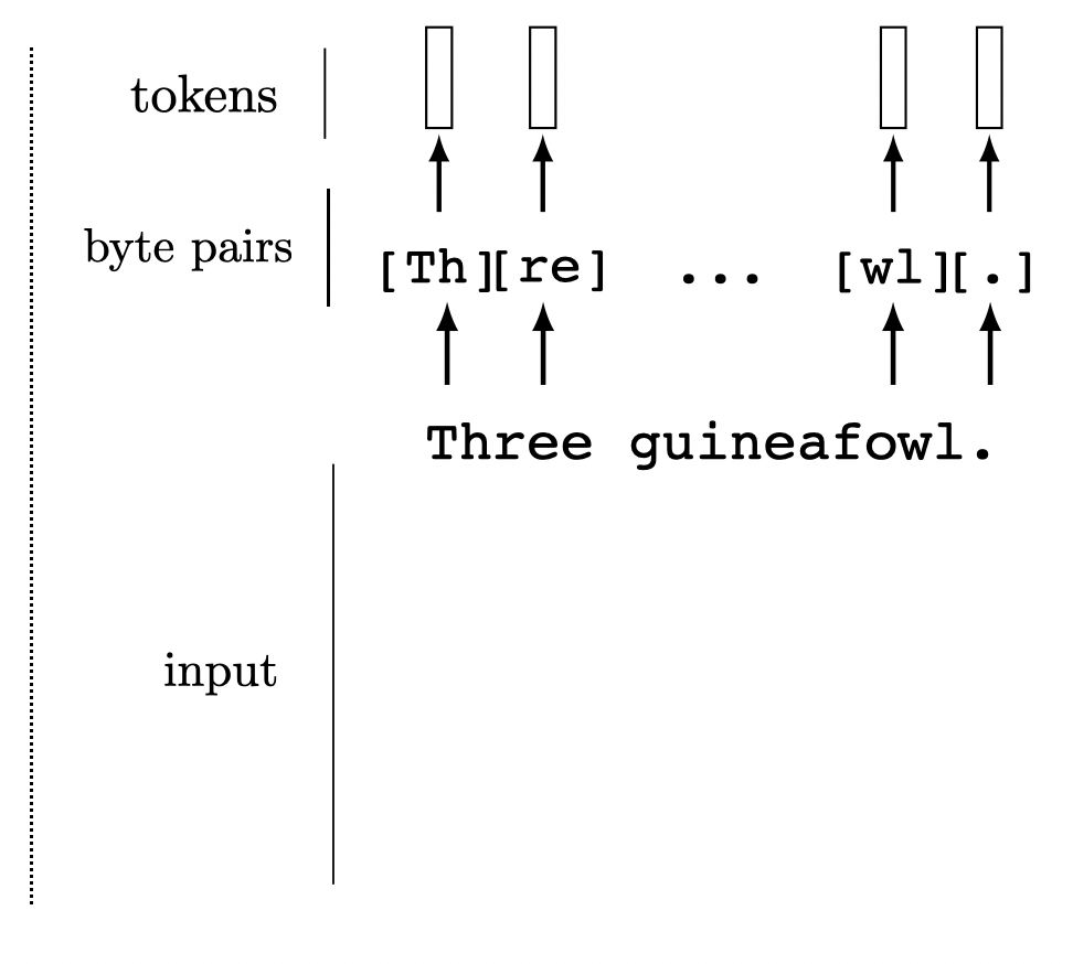
[images credit: visionbook.mit.edu]
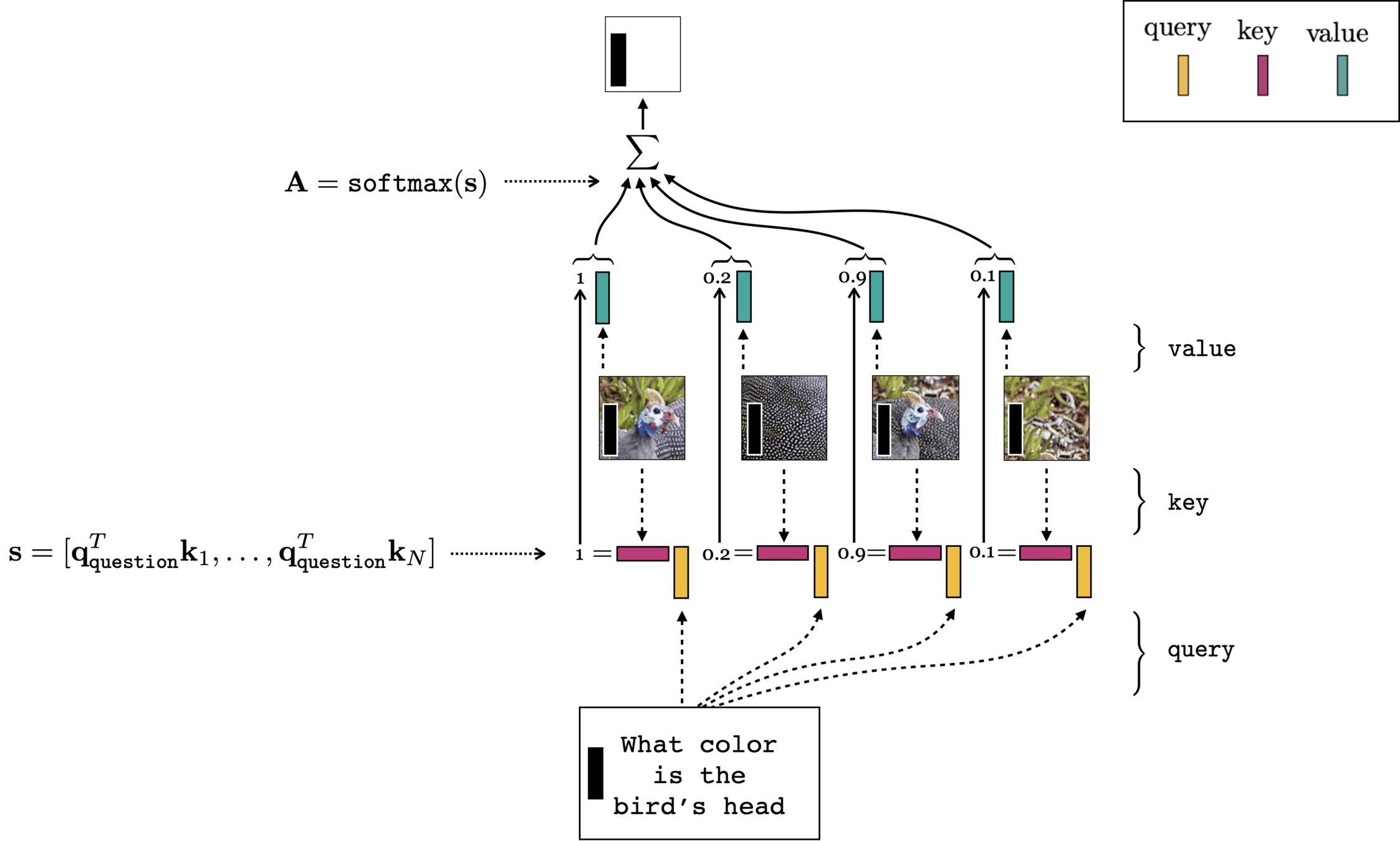
Multi-modality (image q&a)
- (query, key, value) come from different input modality
- cross-attention
[images credit: visionbook.mit.edu]
Biology: attention learns protein structure
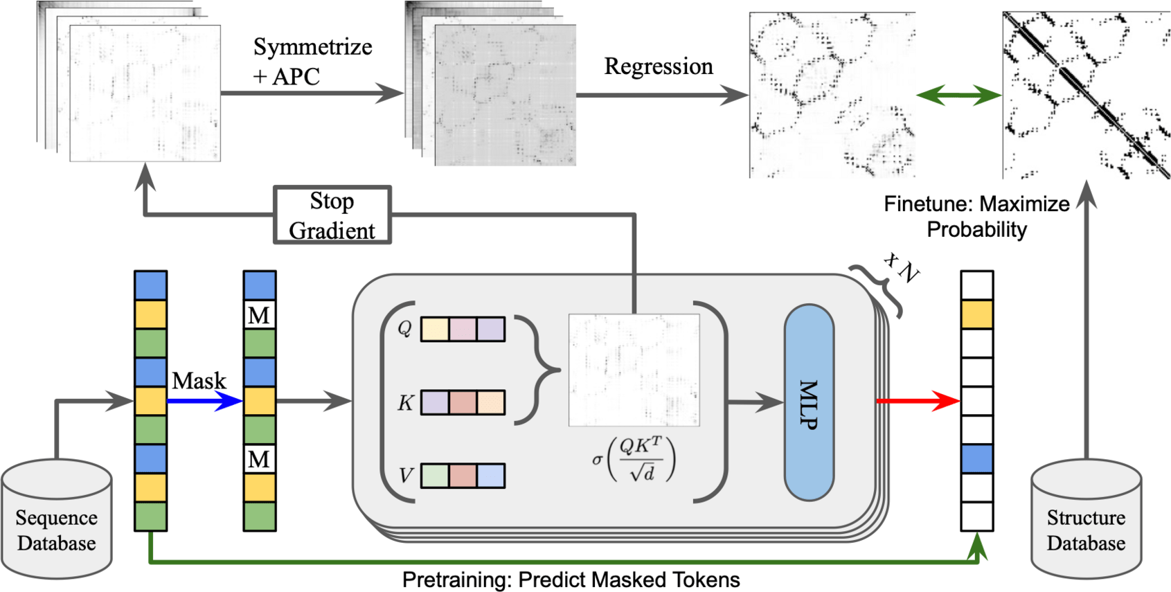
- large \(a_{ij}\) ≈ amino acids \(i\) and \(j\) touch once the protein folds; no one taught it folding
- why it matters: a protein's 3D shape decides what it does (e.g., which drugs bind); sequences are cheap to read, shapes take months to measure in a lab
- ESMFold and AlphaFold predict the full 3D shape from sequence
Attention map highlights objects (DINO)
Attention maps can have artifacts
input
ViT (DINOv2)
same ViT + 4 registers

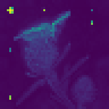
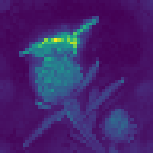
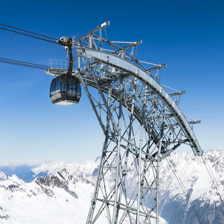
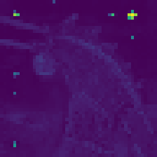
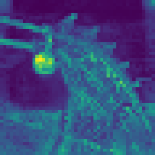
a few background patches get hijacked as scratch memory (bright dots, middle column)
blank "register" tokens give the model scratch space instead, and the maps clean up (right column)
Attention sinks: a big attention score isn't always meaningful
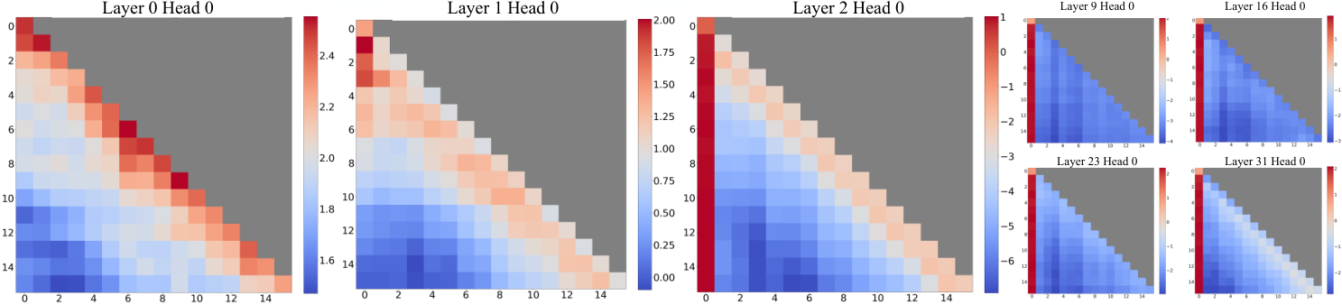
- average attention logits in Llama-2 (grey: masked future)
- each row must hand out 100%; every row can see the first token, so heads park leftover attention there
- so a big \(a_{i1}\) is a parking spot, not importance (like the registers)
- emerged on its own; later models add a dedicated sink token on purpose
Does a head matter? Disable it and check
task: retrieve one fact hidden in a long document
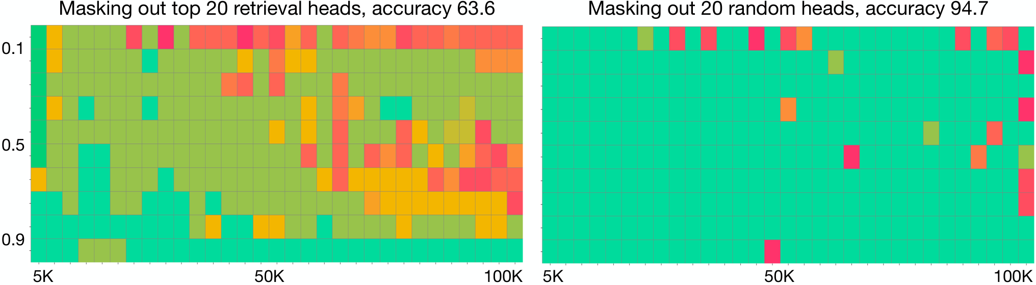
Removing retrieval heads hurts more than removing random heads.
x: document length (5K–100K tokens) · y: where the fact sits (0.1 = start, 0.9 = end) · green = retrieved correctly
TabPFN: no training on your table; it attends to it at prediction time
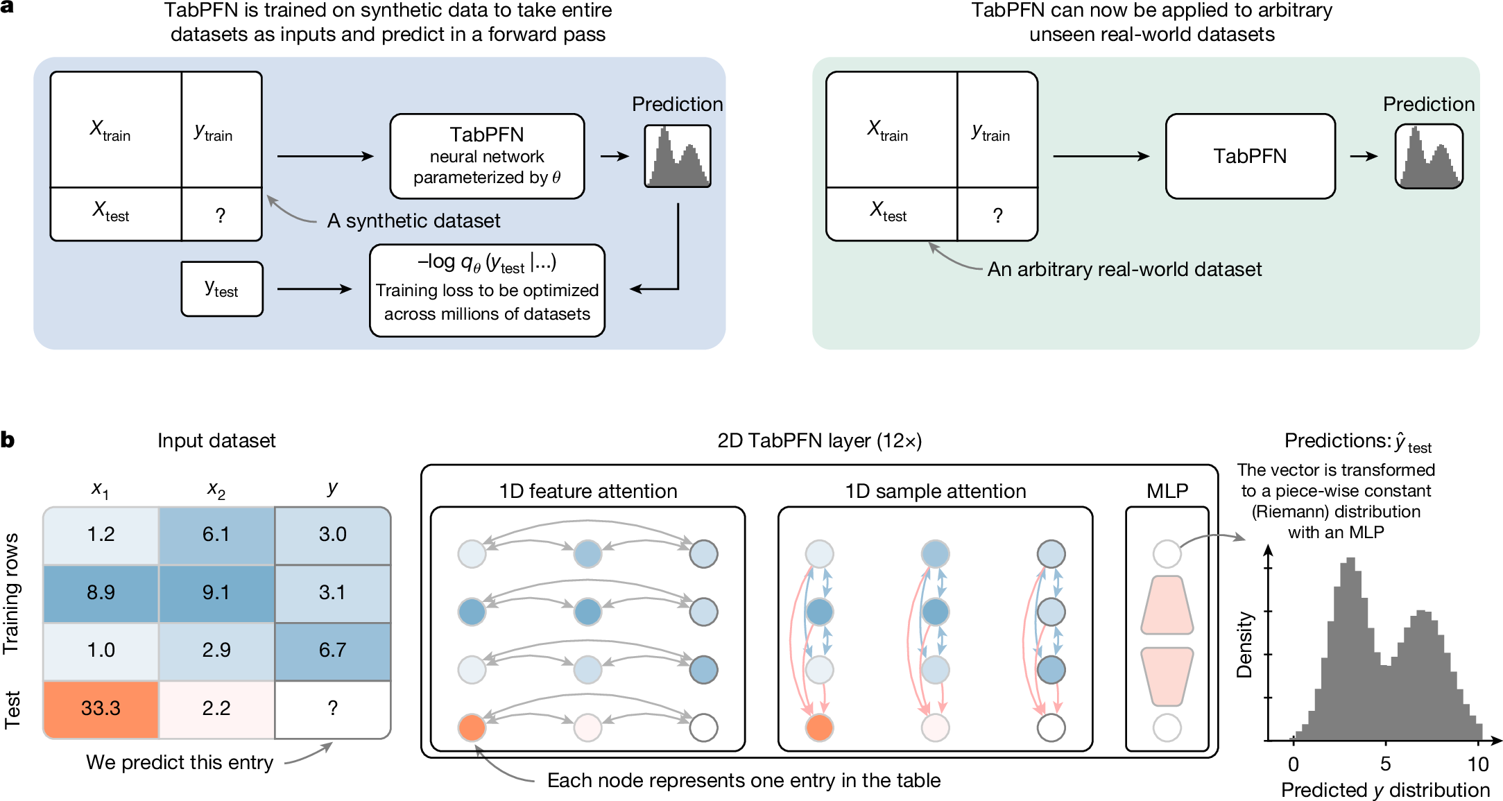
trained once on millions of synthetic tables; on a new table: no training, just one forward pass
test row = query, training rows = keys, their labels = values: the soft dictionary lookup from slide 3
Summary
Attention creates context-aware representations: learned \(\textcolor{#6aa84f}{W_q, W_k, W_v}\) project each token into a query, key, and value; queries and keys set the mixing percentages, values supply what gets combined.
Multiple heads each learn their own \(\textcolor{#6aa84f}{W_q, W_k, W_v}\) and working space \(\mathbb{R}^{d_k}\); \(\textcolor{#6aa84f}{W_o}\) maps the concatenated outputs back to word space \(\mathbb{R}^d\).
Training processes tokens in parallel: causal masking prevents access to future tokens.
Attention extends beyond language: the same mechanism supports vision, proteins, and tabular data.
Human-like concepts emerge in LLMs
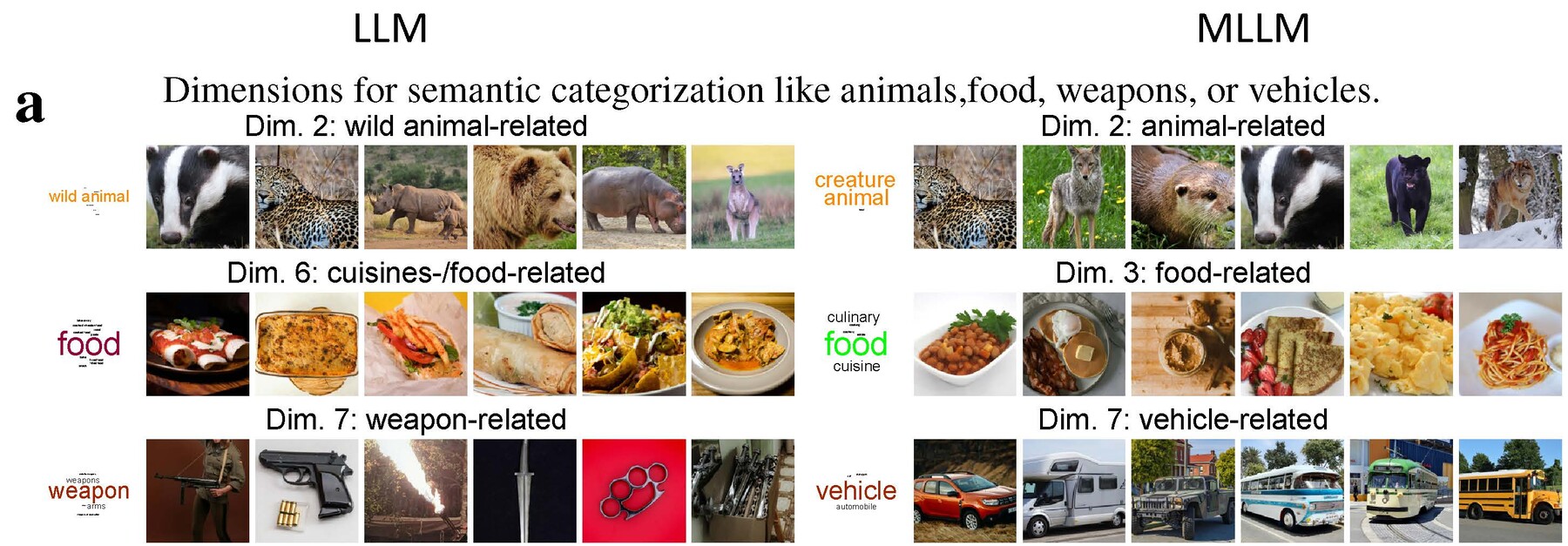
- from 4.7M odd-one-out judgments, each model gets 66 interpretable concept dimensions: animal, food, vehicle, ...
- these line up with human judgments, and with brain activity in category-selective regions
parting thoughts