

Lecture 1: Intro and Linear Regression
Intro to Machine Learning

Medicine
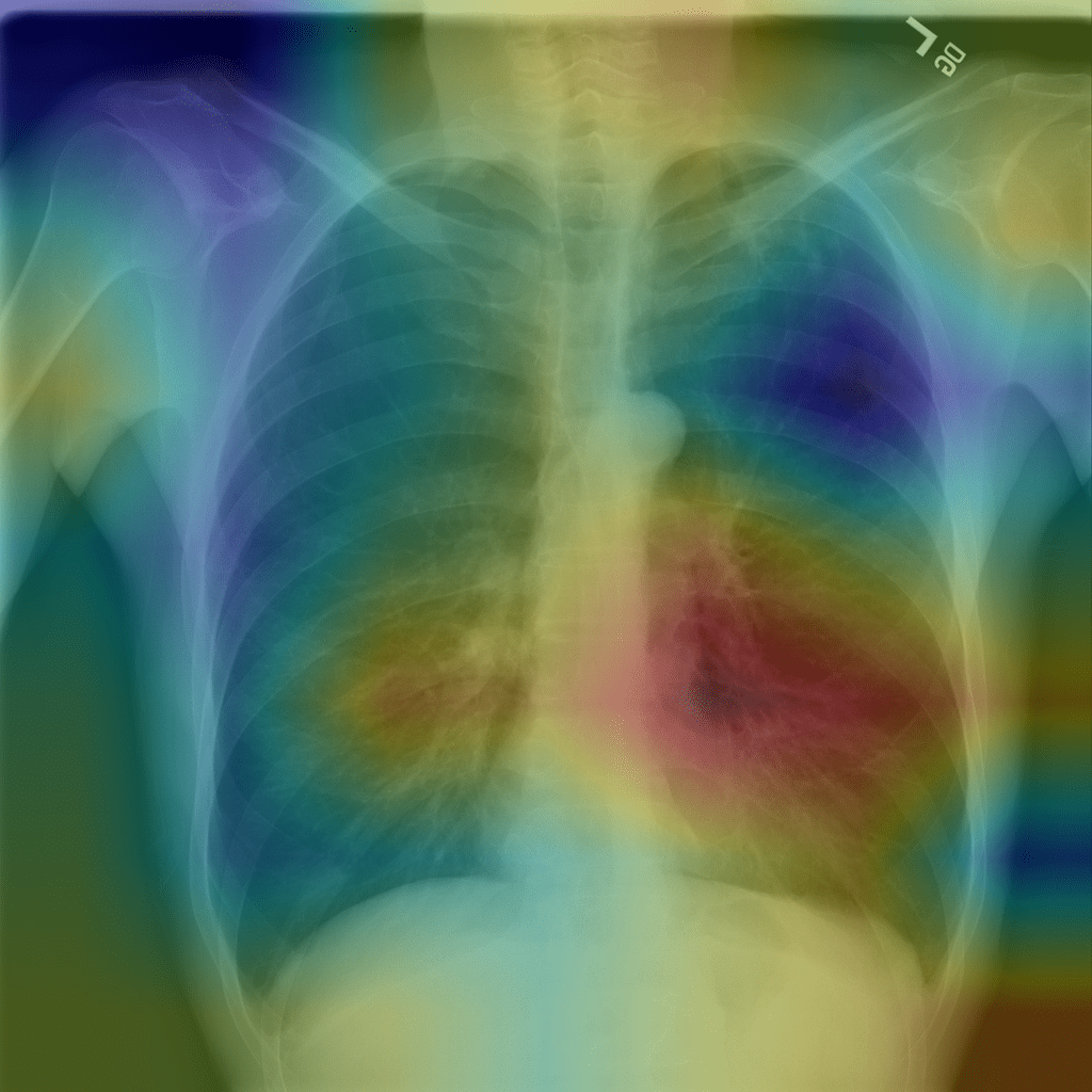
CheXNet (Stanford, 2017)
- An ML system trained on 112K labeled chest X-rays
- Detects pneumonia at radiologist-level accuracy
- Heatmap shows where the model "looks"
Input: X-ray image & label (disease / no disease) →
Output: diagnosis + localization
Science
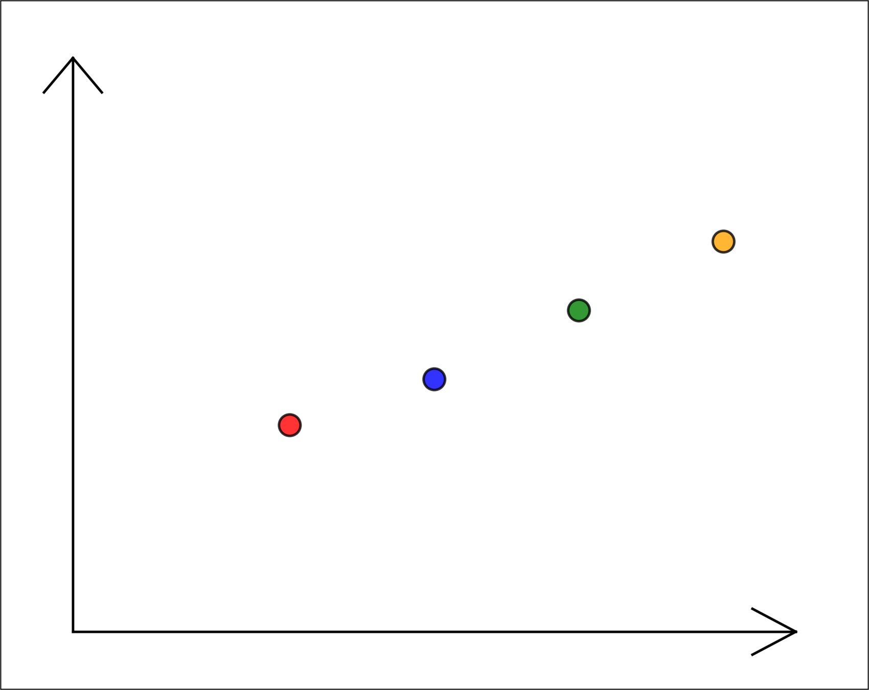
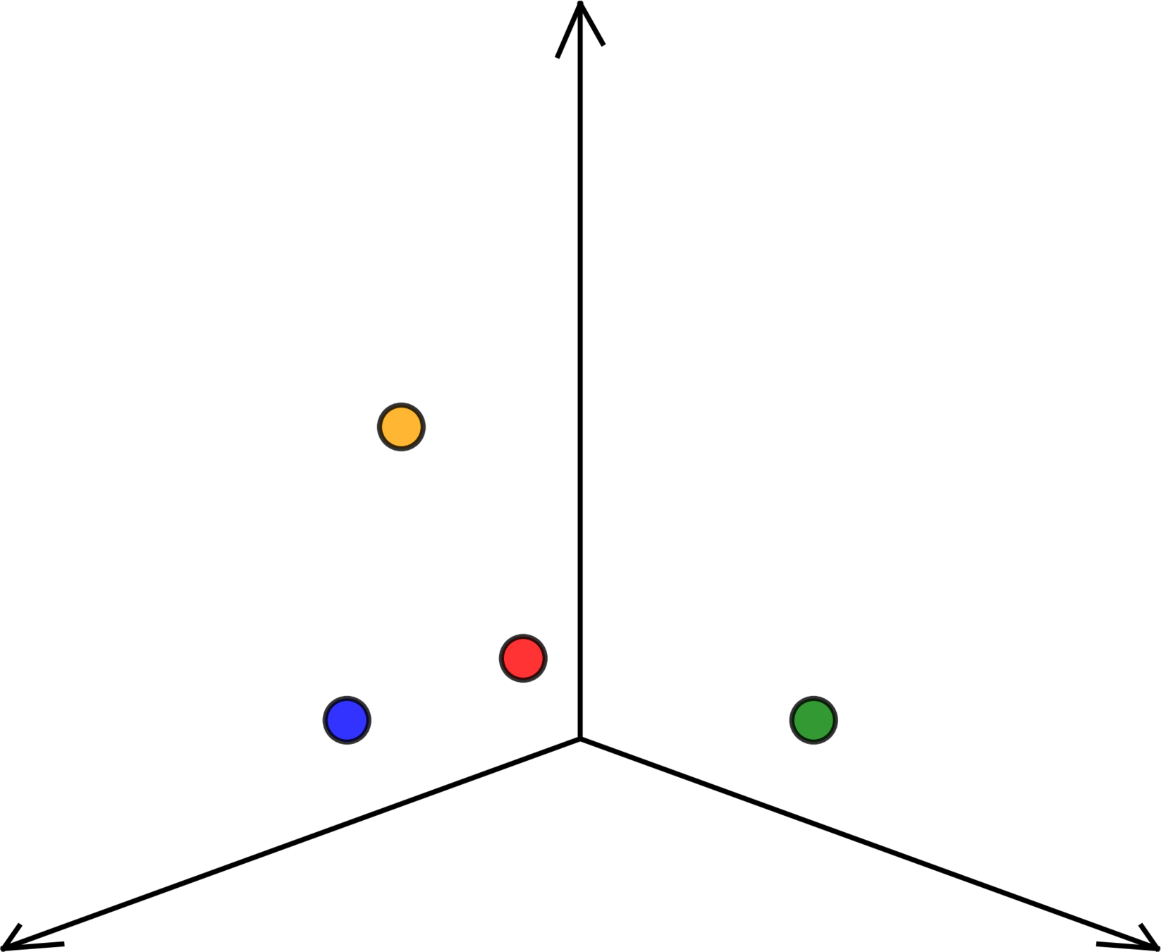
Tabula Sapiens (CZI, 2022)
- 500K+ human cells profiled by gene expression
- Clustering reveals cell types across 24 organs — no predefined labels
- Each dot = one cell; color = organ of origin
Input: gene expression vectors
→ Output: discovered groupings

Robotics
π*0.6 (Physical Intelligence, 2025)
- Vision-language-action model learns from demos + practice
- Makes espresso, folds laundry, assembles boxes
- No task-specific programming — learns by trial and reward
State: camera image → Action: motor commands → Reward: task completion
traditionally
supervised learning
unsupervised learning
reinforcement learning
nowadays
reinforcement learning
supervised learning
unsupervised learning
- self-supervised
- contrastive learning (DALL-E)
behavior cloning
Reinforcement Learning with Human Feedback
(ChatGPT etc.)
Unsupervised skill discovery
In 6.390:
supervised learning
unsupervised learning
reinforcement learning
Outline
- Course overview
- Supervised learning terminologies
- Ordinary least squares regression
- Intro to ML
- Regression and Regularization
- Gradient Descent
- Linear Classification
- Features, Neural Networks I
- Neural Networks II (Backprop)
- Convolutional Neural Networks
- Representation Learning
- Transformers
- Markov Decision Processes
- Reinforcement Learning
- Non-parametric Models
Topics in order:
Many other ways to dissect
Model class:
- linear models
- linear model on non-linear features
- fully connected feed-forward nets
- convolutional nets
- transformers
- Q-table
- tree, k-nearest neighbor, k-means
Optimization:
- analytical solutions
- gradient descent
- back propagation
- value iteration, Q-learning
- non-parametric methods
Learning process:
- training/validation/testing
- overfitting/underfitting
- regularization
- hyper parameters
Modeling choices:
- Supervised:
- regression
- classification
- Unsupervised/self-supervised
- Reinforcement/sequential
[These lists are neither exhaustive nor exclusive.]
After 6.390, you can…
- Frame ML problems: problem class, assumptions, evaluation.
- Build baselines and measure generalization (train vs. test).
- Implement and reason about regression and classification.
- Optimize models with gradients (SGD) and regularization.
- Work with representations and neural networks.
- Understand modern LLM mechanisms (transformers) and MDP/RL basics.
Class meetings
released
due
Hours:
Lec: 1.5 hr
Rec + Lab: 3 hr
Notes + exercise: 2 hr
Homework: 6-7 hr
| Week # | Monday | Tuesday | Wednesday | Thursday | Friday |
| N | Exercise N | Homework N | Exercise N | Recitation N | |
| Lecture N | Lab N | ||||
| N+1 | Homework N | ||||
A typical content week in 6.390:
Grading
- Our objective (and we hope yours) is for you to learn about machine learning — take responsibility for your understanding; we are here to help!
- Grades formula: exercises 5% + homework 20% + labs 15% + midterms 30% + final 30%
- Lateness: 20% penalty per day, applied linearly (so 1 hour late is -0.83%)
- 20 one-day extensions, applied automatically on May 13 to maximize your benefit
- Midterm 1: Thursday, March 12, 7:30–9pm
- Midterm 2: Wednesday, April 15, 7:30–9pm
- Final: scheduled by Registrar (posted in 3rd week). ⚠️ – might be as late as May 21!
Collaboration and How to Get Help
- Understand everything you turn in
- Coding and detailed derivations must be done by you
- See collaboration policy/examples on course web site
- Office hours: lots! (Starting this Thursday)
- See Google Calendar for holiday/schedule shift
- Make use of Piazza and Pset-partners
- Logistic, personal issues, reach out to
6.390-personal@mit.edu (looping in S^3 and/or DAS)
Outline
- Course overview
- Supervised learning terminologies
- Ordinary least squares regression
an instance supervised learning known as regression: predicting a continuous number
e.g., want to predict a city's energy usage
temperature \(x\)
energy used \(y\)
toy data, for illustration only
| City | Feature | Label |
|---|---|---|
| Temperature | Energy Used | |
| Chicago | 90 | 45 |
| New York | 20 | 32 |
| Boston | 35 | 99 |
| San Diego | 18 | 39 |
go collect some data in various cities
temperature \(x\)
energy used \(y\)
\(\left\{\left(x^{(1)}, y^{(1)}\right), \dots, \left(x^{(4)}, y^{(4)}\right)\right\}\)
\(\mathcal{D}_\text{train}:=\)
\(x^{(1)} \in \mathbb{R}\)
label
feature
\(y^{(1)} \in \mathbb{R}\)
\((x^{(1)}, y^{(1)})\)
Training data:
\(x^{(1)} =\begin{bmatrix} x_1^{(1)} \\[4pt] x_2^{(1)} \end{bmatrix} \in \mathbb{R}^2\)
label
feature vector
\(y^{(1)} \in \mathbb{R}\)
\(\mathcal{D}_\text{train}:=\)
\(\left\{\left(x^{(1)}, y^{(1)}\right), \dots, \left(x^{(4)}, y^{(4)}\right)\right\}\)
\((x^{(1)}, y^{(1)})\)
\(=\left(\begin{bmatrix} x_1^{(1)} \\[4pt] x_2^{(1)} \\[4pt] \end{bmatrix}, y^{(1)}\right)\)
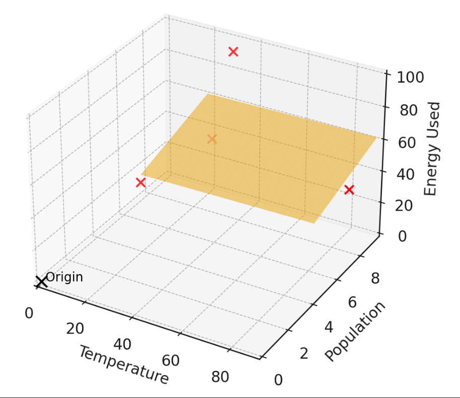
temperature \(x_1\)
population \(x_2\)
energy used \(y\)
Training data:
\(x^{(1)} =\begin{bmatrix} x_1^{(1)} \\[4pt] x_2^{(1)} \\[4pt] \vdots \\[4pt] x_d^{(1)} \end{bmatrix} \in \mathbb{R}^d\)
label
feature vector
\(y^{(1)} \in \mathbb{R}\)
\(\mathcal{D}_\text{train}:=\)
\(\left\{\left(x^{(1)}, y^{(1)}\right), \dots, \left(x^{(n)}, y^{(n)}\right)\right\}\)
\(n = 4, d = 1\)
\(n = 4 ,d = 2\)
temperature \(x_1\)
energy used \(y\)
temperature \(x_1\)
population \(x_2\)
energy used \(y\)
\(n\) data points, each with \(d\)-dimensional features and scalar label
Training data:
Training data in matrix-vector form:
temperature \(x\)
energy used \(y\)
| City | Feature | Label |
|---|---|---|
| Temperature | Energy Used | |
| Chicago | 90 | 45 |
| New York | 20 | 32 |
| Boston | 35 | 99 |
| San Diego | 18 | 39 |
\(X = \begin{bmatrix} {\color{#cc0000}{90}} \\ {\color{#0000cc}{20}} \\ {\color{#009900}{35}} \\ {\color{#cc9900}{18}} \end{bmatrix}\)
\(Y = \begin{bmatrix} {\color{#cc0000}{45}} \\ {\color{#0000cc}{32}} \\ {\color{#009900}{99}} \\ {\color{#cc9900}{39}} \end{bmatrix}\)
\(\in \mathbb{R}^{4 \times 1}\)
\(\in \mathbb{R}^{4 \times 1}\)
temperature \(x_1\)
population \(x_2\)
energy used \(y\)
| City | Features | Label | |
|---|---|---|---|
| Temperature | Population | Energy Used | |
| Chicago | 90 | 7.2 | 45 |
| New York | 20 | 9.5 | 32 |
| Boston | 35 | 8.4 | 99 |
| San Diego | 18 | 4.3 | 39 |
\(X = \begin{bmatrix} {\color{#cc0000}{90}} & {\color{#cc0000}{7.2}} \\ {\color{#0000cc}{20}} & {\color{#0000cc}{9.5}} \\ {\color{#009900}{35}} & {\color{#009900}{8.4}} \\ {\color{#cc9900}{18}} & {\color{#cc9900}{4.3}} \end{bmatrix}\)
\(\in \mathbb{R}^{4 \times 2}\)
\(Y = \begin{bmatrix} {\color{#cc0000}{45}} \\ {\color{#0000cc}{32}} \\ {\color{#009900}{99}} \\ {\color{#cc9900}{39}} \end{bmatrix}\)
\(\in \mathbb{R}^{4 \times 1}\)
Regression
Algorithm
💻
\(\in \mathbb{R}^d \)
\(\in \mathbb{R}\)
\(\mathcal{D}_\text{train}\)
What do we want from the regression algortim?
A good way to label new features, i.e. a good hypothesis.
hypothesis
Learning algorithm spits out a hypothesis
- Loss
\(\mathcal{L}\left(h\left(x^{(i)}\right), y^{(i)}\right) \)
temperature \(x\)
\(h(x)=10\)
e.g. \(h\left(x^{(4)}\right) - y^{(4)} \)
energy used \(y\)
\(\mathcal{E}_{\text {train }}(h)=\frac{1}{n} \sum_{i=1}^n \mathcal{L}\left(h\left(x^{(i)} \right), y^{(i)}\right)\)
- Training error
\(\mathcal{E}_{\text {test }}(h)=\frac{1}{n^{\prime}} \sum_{i=n+1}^{n+n^{\prime}} \mathcal{L}\left(h\left(x^{(i)}\right), y^{(i)}\right)\)
- Test error
i.e. average loss on \(n'\) unseen test data points
set of \(h\) we ask the algorithm to search over
Hypothesis class \(\mathcal{H}:\)
\(\{\)constant functions\(\}\)
temperature \(x\)
energy used \(y\)
\(\subset\)
less expressive
more expressive
\(\{\)linear functions\(\}_1\)
1. technically, affine functions. ML community tends to be flexible about this terminology.
\(h_1(x)=10\)
\(h_2(x)=20\)
\(h_3(x)=30\)
temperature \(x\)
energy used \(y\)
\(h(x)=3x -5\)
\(h(x)=4x +2\)
Regression
Algorithm
💻
\(\in \mathbb{R}^d \)
\(\in \mathbb{R}\)
\(\mathcal{D}_\text{train}\)
🧠 ⚙️
- hypothesis class
- loss function
Quick summary:
Classification
Algorithm
💻
🧠⚙️
hypothesis class
loss function
...
classifier
{"Fish", "Grizzly", "Chameleon", ...}
"Fish"

images adapted from Phillip Isola
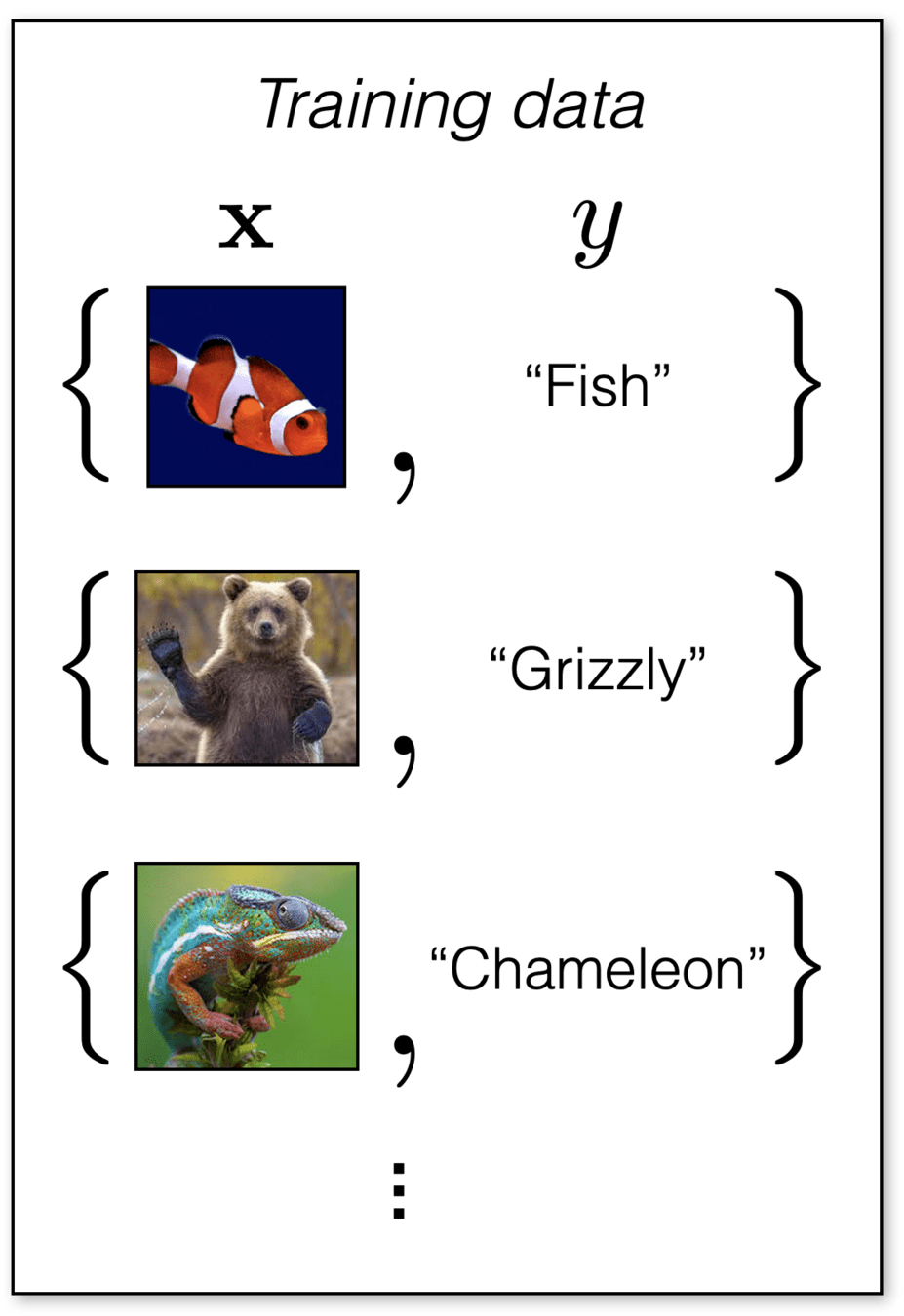
features
label
Looking ahead:
Outline
- Course overview
- Supervised learning terminologies
- Ordinary least squares regression
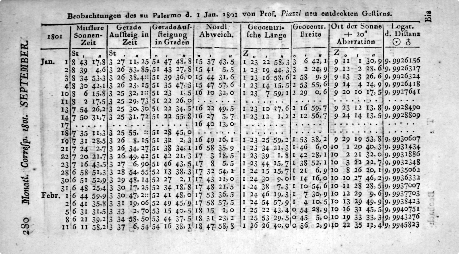
Why least squares?
- Problem: infer orbit parameters from noisy, partial measurements.
- Idea: pick parameters that make predictions match observations as closely as possible, by minimize the sum of squared residuals.
- Today: still a fast, reliable, interpretable baseline.
Primary source: Gauss, Theoria motus (1809).
Observation table: Piazzi’s measurements of Ceres (1801).

Regression
Algorithm
💻
\(\in \mathbb{R}^d \)
\(\in \mathbb{R}\)
\(\mathcal{D}_\text{train}\)
🧠 ⚙️
- hypothesis class
- loss function
General regression
Closed-form formula
💻
\(\in \mathbb{R}^d \)
\(\in \mathbb{R}\)
\(\mathcal{D}_\text{train}\)
🧠 ⚙️
- linear hypothesis class
- squared loss function
Ordinary least squares regression
Linear hypothesis class:
\(h\left(x ; \theta\right)\)
\( = \left[\begin{array}{lllll} \theta_1 & \theta_2 & \cdots & \theta_d\end{array}\right]\) \(\left[\begin{array}{c} x_1 \\ x_2 \\ \vdots \\ x_d\end{array}\right]\)
parameters
Squared loss function:
\(\mathcal{L}\left(h\left(x^{(i)}\right), y^{(i)}\right) =(\theta^T x^{(i)}- y^{(i)} )^2\)
temperature \(x_1\)
population \(x_2\)
energy used \(y\)
for now, ignoring the offset
\(=\)
\(x\)
\(\theta^T\)
features
Ordinary least squares regression
Deriving the OLS solution
- Write the training error \(J(\theta)\) in scalar form
- Rearrange into matrix-vector form
- Set the gradient \(\nabla_\theta J\) to zero
- Solve for the optimal parameters
Note: step 3 \(\rightarrow\) 4 (\(\nabla_\theta J(\theta) = 0 \implies \theta\text{ is a minimizer}\)) isn't always true in general. We'll discuss when this implication breaks in Week 3.
\( J(\theta) =\frac{1}{n}({X} \theta-{Y})^{\top}({X} \theta-{Y})\)
\(\theta^*=\left({X}^{\top} {X}\right)^{-1} {X}^{\top} {Y}\)
\( J(\theta) = \frac{1}{4}\big[ ({\theta_1} \cdot {\color{#cc0000}{90}} + {\theta_2} \cdot {\color{#cc0000}{7.2}} - {\color{#cc0000}{45}})^2 + ({\theta_1} \cdot {\color{#0000cc}{20}} + {\theta_2} \cdot {\color{#0000cc}{9.5}} - {\color{#0000cc}{32}})^2 + ({\theta_1} \cdot {\color{#009900}{35}} + {\theta_2} \cdot {\color{#009900}{8.4}} - {\color{#009900}{99}})^2 + ({\theta_1} \cdot {\color{#cc9900}{18}} + {\theta_2} \cdot {\color{#cc9900}{4.3}} - {\color{#cc9900}{39}})^2 \big]\)
| City | Features | Label | |
|---|---|---|---|
| Temp (°F) | Pop (M) | Energy (kWh) | |
| Chicago | 90 | 7.2 | 45 |
| New York | 20 | 9.5 | 32 |
| Boston | 35 | 8.4 | 99 |
| San Diego | 18 | 4.3 | 39 |
1. Write out training error:
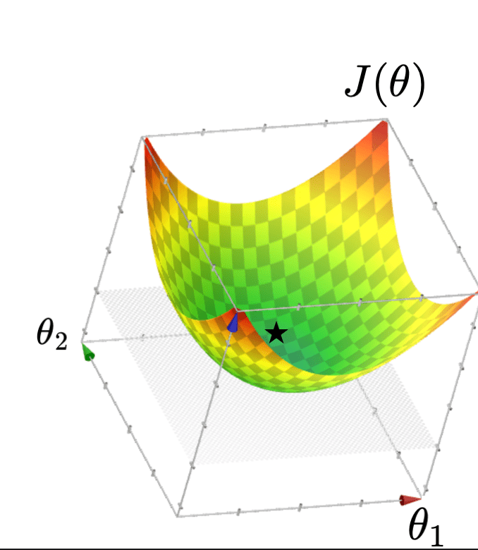
- Q: What kind of function is \(J(\theta)\)?
- A: Quadratic function
- Q: What does \(J(\theta)\) look like?
- A: Typically, looks like a "bowl"
e.g.:
\(\theta = \begin{bmatrix} \theta_1 \\ \theta_2 \end{bmatrix}\)
\(\in \mathbb{R}^{2 \times 1}\)
\(X = \begin{bmatrix} \color{#cc0000}{90} & \color{#cc0000}{7.2} \\ \color{#0000cc}{20} & \color{#0000cc}{9.5} \\ \color{#009900}{35} & \color{#009900}{8.4} \\ \color{#cc9900}{18} & \color{#cc9900}{4.3} \end{bmatrix}\)
\(\in \mathbb{R}^{4 \times 2}\)
\(Y = \begin{bmatrix} \color{#cc0000}{45} \\ \color{#0000cc}{32} \\ \color{#009900}{99} \\ \color{#cc9900}{39} \end{bmatrix}\)
\( J(\theta) = \frac{1}{4}\big[ ({\theta_1} \cdot {\color{#cc0000}{90}} + {\theta_2} \cdot {\color{#cc0000}{7.2}} - {\color{#cc0000}{45}})^2 + ({\theta_1} \cdot {\color{#0000cc}{20}} + {\theta_2} \cdot {\color{#0000cc}{9.5}} - {\color{#0000cc}{32}})^2 + ({\theta_1} \cdot {\color{#009900}{35}} + {\theta_2} \cdot {\color{#009900}{8.4}} - {\color{#009900}{99}})^2 + ({\theta_1} \cdot {\color{#cc9900}{18}} + {\theta_2} \cdot {\color{#cc9900}{4.3}} - {\color{#cc9900}{39}})^2 \big]\)
\(\theta = \begin{bmatrix} \theta_1 \\ \theta_2 \end{bmatrix}\)
\(\in \mathbb{R}^{4 \times 1}\)
\(\in \mathbb{R}^{2 \times 1}\)
\( J(\theta) =\frac{1}{n}({X} \theta-{Y})^{\top}({X} \theta-{Y})\)
| City | Features | Label | |
|---|---|---|---|
| Temp (°F) | Pop (M) | Energy (kWh) | |
| Chicago | 90 | 7.2 | 45 |
| New York | 20 | 9.5 | 32 |
| Boston | 35 | 8.4 | 99 |
| San Diego | 18 | 4.3 | 39 |
2. Rearrange training error into matrix-vector form
- Typically, \(J(\theta)\) "curves up"
- The minimizer of \(J(\theta)\) necessarily has a gradient zero.
3. Get the gradient \(\nabla_\theta J\stackrel{\text { set }}{=} 0\)
\(\nabla_\theta J=\left[\begin{array}{c}\partial J / \partial \theta_1 \\ \vdots \\ \partial J / \partial \theta_d\end{array}\right]\)
= \(\frac{2}{n}\left(X^T X \theta-X^T Y\right)\)
\(\theta^*=\left({X}^{\top} {X}\right)^{-1} {X}^{\top} {Y}\)
4. Set the gradient \(\nabla_\theta J\stackrel{\text { set }}{=} 0\)
- When \(\theta^*\) is well defined, it's the unique minimizer of \(J(\theta\))
- Closed-form solution, does not feel like "training"
- Very rare case where we get a general and clean solution with nice theoretical guarantee.
The beauty of
\(\theta^*=\left({X}^{\top} {X}\right)^{-1} {X}^{\top} {Y}\)
Summary
- Terminologies:
- Ordinary least squares regression:
- linear hypothesis class, squared loss, mean-squared error
- matrix-vector form objective
- closed-form solution
\( J(\theta) =\frac{1}{n}({X} \theta-{Y})^{\top}({X} \theta-{Y})\)
\(\theta^*=\left({X}^{\top} {X}\right)^{-1} {X}^{\top} {Y}\)
- When is this \(\theta^*\) not well defined?
- What can cause this "not well defined"?
- What happens if we are just "close to not well-defined", aka "ill-conditioned"?
- We'll discuss all these next week.
When \(\theta^*\) is well defined, it's the unique minimizer of \(J(\theta\))
\(\theta^*=\left({X}^{\top} {X}\right)^{-1} {X}^{\top} {Y}\)
Looking ahead:
Thanks!
We'd love to hear your thoughts.
Reference: Gradient Vector Refresher
(5 important facts for 6.390)
For \(f: \mathbb{R}^m \rightarrow \mathbb{R}\), its gradient \(\nabla f: \mathbb{R}^m \rightarrow \mathbb{R}^m\) is defined at the point \(p=\left(x_1, \ldots, x_m\right)\) as:
Sometimes the gradient is undefined or ill-behaved, but today it is well-behaved.
- The gradient generalizes the concept of a derivative to multiple dimensions.
- By construction, the gradient's dimensionality always matches the function input.
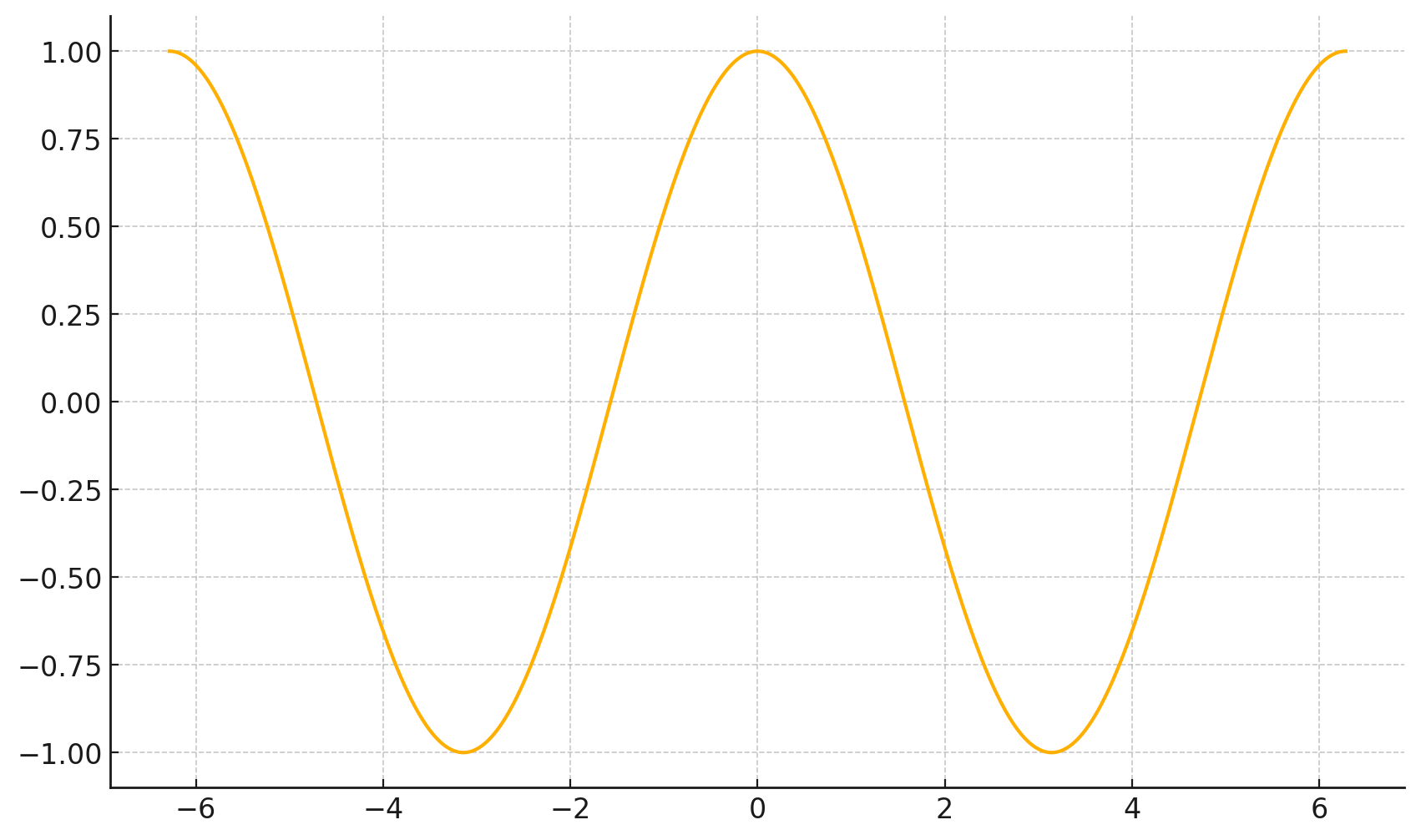
3. The gradient can be symbolic or numerical.
example:
its symbolic gradient:
just like a derivative can be a function or a number.
evaluating the symbolic gradient at a point gives a numerical gradient:
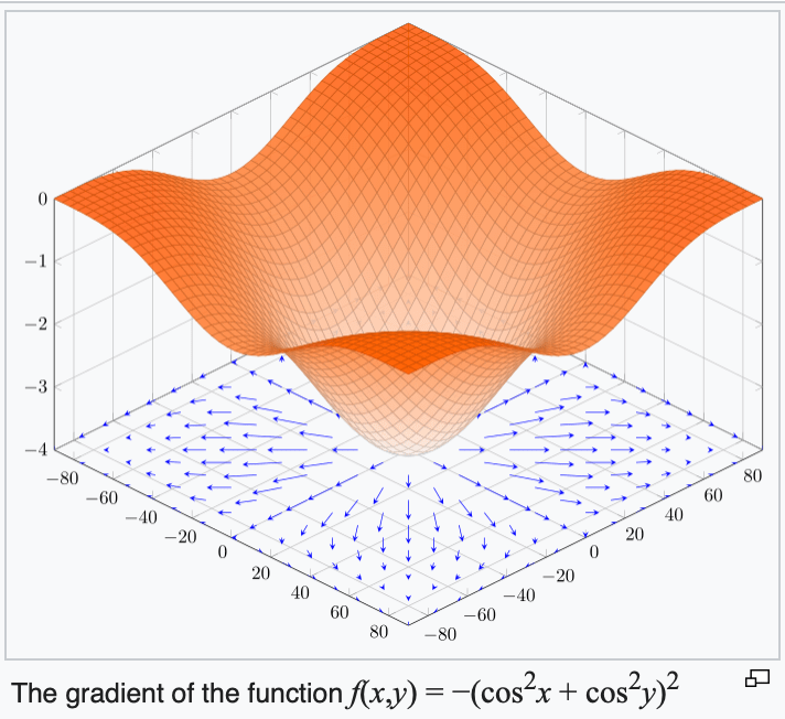
4. The gradient points in the direction of the (steepest) increase in the function value.
\(\frac{d}{dx} \cos(x) \bigg|_{x = -4} = -\sin(-4) \approx -0.7568\)
\(\frac{d}{dx} \cos(x) \bigg|_{x = 5} = -\sin(5) \approx 0.9589\)
5. The gradient at the function minimizer is necessarily zero.
For \(f: \mathbb{R}^m \rightarrow \mathbb{R}\), its gradient \(\nabla f: \mathbb{R}^m \rightarrow \mathbb{R}^m\) is defined at the point \(p=\left(x_1, \ldots, x_m\right)\) as:
Sometimes the gradient is undefined or ill-behaved, but today it is well-behaved.
- The gradient generalizes the concept of a derivative to multiple dimensions.
- By construction, the gradient's dimensionality always matches the function input.
- The gradient can be symbolic or numerical.
- The gradient points in the direction of the (steepest) increase in the function value.
- The gradient at the function minimizer is necessarily zero.
Extension: How to deal with offset \(\theta_0\)
- center the data; or
- append a fake feature of 1
1. "center" the data
when data is centered, the optimal offset is guaranteed to be 0
centering
| Features | Label | ||
|---|---|---|---|
| City | Temperature | Population | Energy Used |
| Chicago | 90 | 7.2 | 45 |
| New York | 20 | 9.5 | 32 |
| Boston | 35 | 8.4 | 100 |
| San Diego | 18 | 4.3 | 39 |
| Features | Label | ||
|---|---|---|---|
| City | Temperature | Population | Energy Used |
| Chicago | 49.25 | -0.15 | -9.00 |
| New York | -20.75 | 2.15 | -22.00 |
| Boston | -5.75 | 1.05 | 46.00 |
| San Diego | -22.75 | -3.05 | -15.00 |
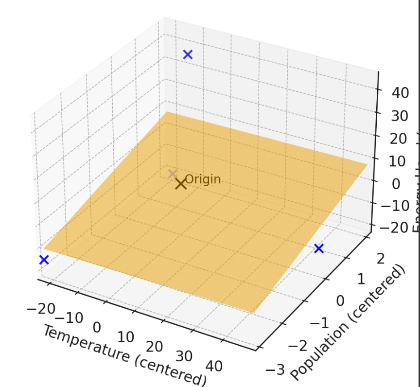
all column-wise \(\Sigma =0\)

2. Append a "fake" feature of \(1\)
\(h\left(x ; \theta, \theta_0\right)=\theta^T x+\theta_0\)
\( = \left[\begin{array}{lllll} \theta_1 & \theta_2 & \cdots & \theta_d\end{array}\right]\) \(\left[\begin{array}{l}x_1 \\ x_2 \\ \vdots \\ x_d\end{array}\right] + \theta_0\)
\( = \left[\begin{array}{lllll} \theta_1 & \theta_2 & \cdots & \theta_d & \theta_0\end{array}\right]\) \(\left[\begin{array}{c}x_1 \\ x_2 \\ \vdots \\ x_d \\ 1\end{array}\right] \)
\( = \theta_{\mathrm{aug}}^T x_{\mathrm{aug}}\)
trick our model: treat the bias as just another feature, always equal to 1.
See recitation 1 for details.
temperature \(x_1\)
energy used \(y\)