6.390 IntroML (Spring26) - Lecture 2 Regularization and Cross-validation

Recall

\(\theta^*=\left({X}^{\top} {X}\right)^{-1} {X}^{\top} {Y}\)

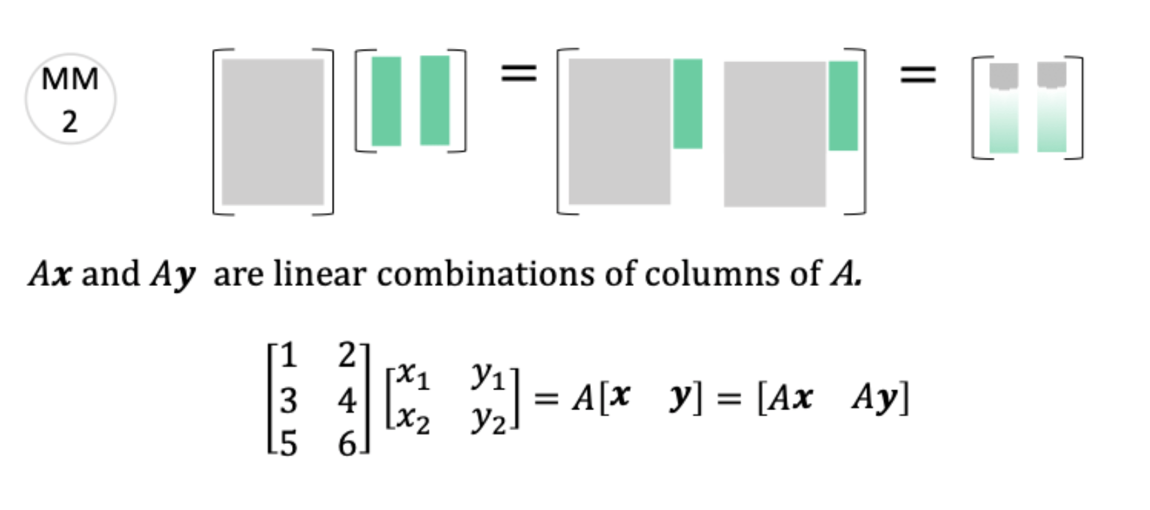
\(X = \begin{bmatrix} \text{---} \; {x^{(1)}}^\top \; \text{---} \\ \vdots \\ \text{---} \; {x^{(n)}}^\top \; \text{---} \end{bmatrix} = \begin{bmatrix} x_1^{(1)} & \cdots & x_d^{(1)} \\ \vdots & \ddots & \vdots \\ x_1^{(n)} & \cdots & x_d^{(n)} \end{bmatrix}\)

\(Y = \begin{bmatrix}y^{(1)}\\\vdots\\y^{(n)}\end{bmatrix}\)

\(\theta = \begin{bmatrix}\theta_{1}\\\vdots\\\theta_{d}\end{bmatrix}\)

\( J(\theta) =\frac{1}{n}({X} \theta-{Y})^{\top}({X} \theta-{Y})\)

Let

Then

\(\in \mathbb{R}^{n\times d}\)

\(\in \mathbb{R}^{n\times 1}\)

\(\in \mathbb{R}^{d\times 1}\)

\(\in \mathbb{R}^{1\times 1}\)

By matrix calculus and optimization

\(\in \mathbb{R}^{d\times 1}\)

\(\theta^*=\left({X}^{\top} {X}\right)^{-1} {X}^{\top} {Y}\)

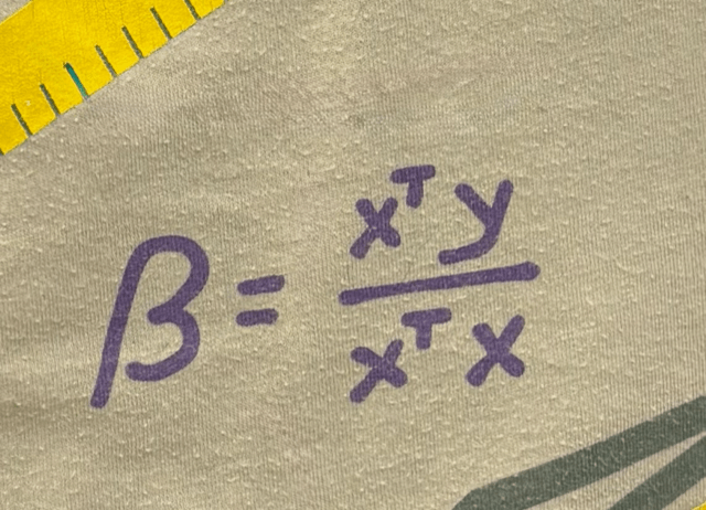
Jane street shirt

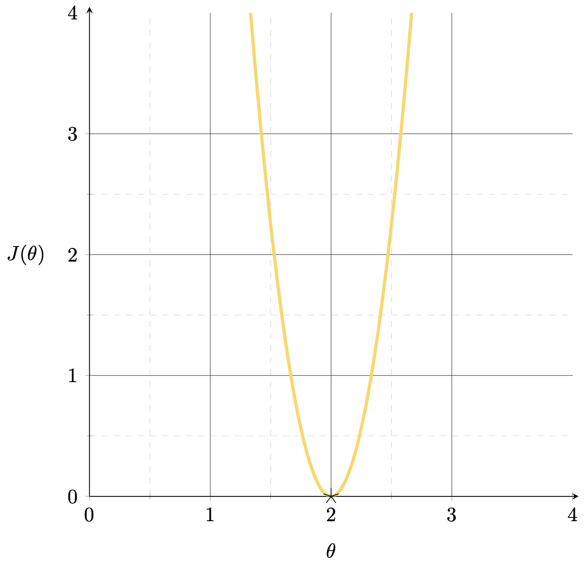
\(J(\theta) = (3 \theta-6)^{2}\)

\(X= [3]\)

\(Y= [6]\)

\(\theta^*=\left({X}^{\top} {X}\right)^{-1} {X}^{\top} {Y}\)

\(\theta^*=(X^\top X)^{-1}(X^\top Y)\)

\(=\frac{X^\top Y}{X^\top X}= \frac{6}{3}=2\)

\(\theta^*\)

J(\theta) = \frac{1}{2}\left[(\theta-3)^2+(2\theta-6)^{2}\right]

\(\theta^*\)

\(X = \begin{bmatrix}1 \\2\end{bmatrix}\)

\(Y = \begin{bmatrix}3 \\6\end{bmatrix}\)

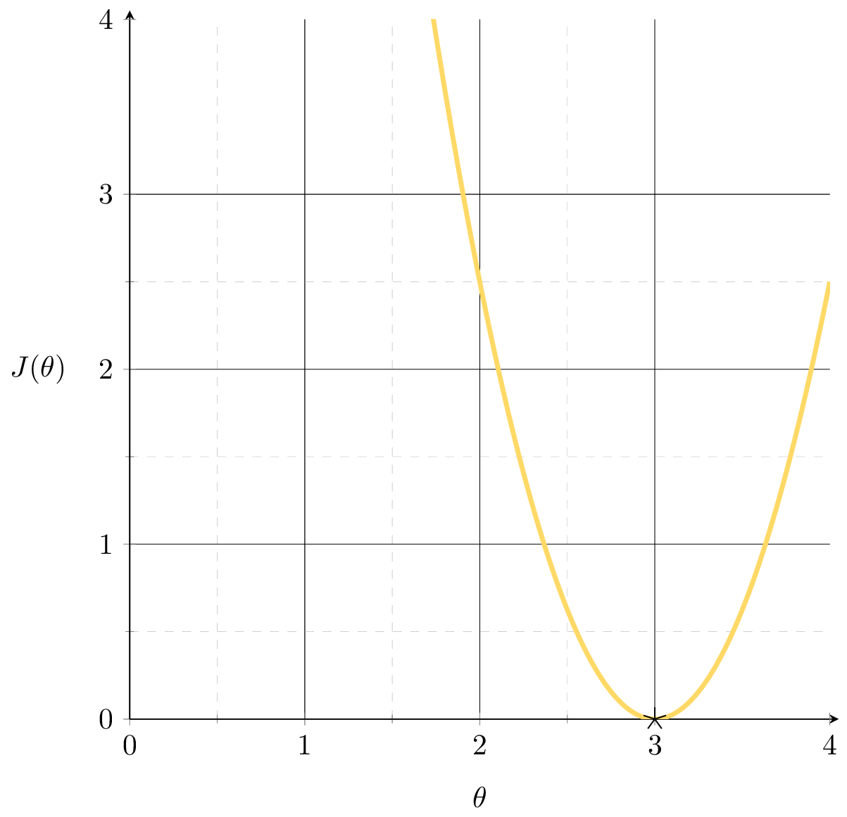
\(=\frac{X^{\top}Y}{X^{\top}X}= \frac{15}{5}= 3\)

\(\theta^*=(X^\top X)^{-1}(X^\top Y)\)

\(\theta^*=\left({X}^{\top} {X}\right)^{-1} {X}^{\top} {Y}\)

\(X = \begin{bmatrix}1 & 0 \\0 & 1 \\ 1 & 1\end{bmatrix}\quad Y = \begin{bmatrix}2 \\3 \\ 5\end{bmatrix}\)

\(X^\top X = \begin{bmatrix}2 & 1 \\1 & 2\end{bmatrix}\quad X^\top Y = \begin{bmatrix}7 \\8\end{bmatrix}\)

\(\theta^* = \begin{bmatrix}2 & 1 \\1 & 2\end{bmatrix}^{-1} \begin{bmatrix}7 \\8\end{bmatrix} = \begin{bmatrix}2 \\3\end{bmatrix}\)

\(\theta^*=\left({X}^{\top} {X}\right)^{-1} {X}^{\top} {Y}\)

Outline

The "trouble" with the closed-form solution
- visually, practically, mathematically
Regularization and ridge regression
Cross-validation

\(\infty\) many optimal \(\theta^*\)

temperature \(x_1\)

population \(x_2\)

energy used

\(y\)

temperature ( °F) \(x_1\)

temperature (°C) \(x_2\)

energy used

\(y\)

data

MSE

\(\theta^*=\left({X}^{\top} {X}\right)^{-1} {X}^{\top} {Y}\)

undefined

(a) \(n < d\)

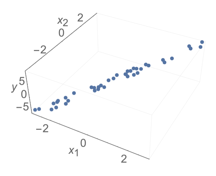
(b) Linearly-dependent features:

closed-form formula

optimal solution

Not enough info to pin down a unique solution

e.g. genomics, NLP

e.g. temp °F/°C, age/birth_year, ...

https://github.com/kenjihiranabe/The-Art-of-Linear-Algebra

https://www.3blue1brown.com/topics/linear-algebra

\(\left({X}^{\top} {X}\right)\) is singular

\({X}\) is not full column rank

\Leftrightarrow

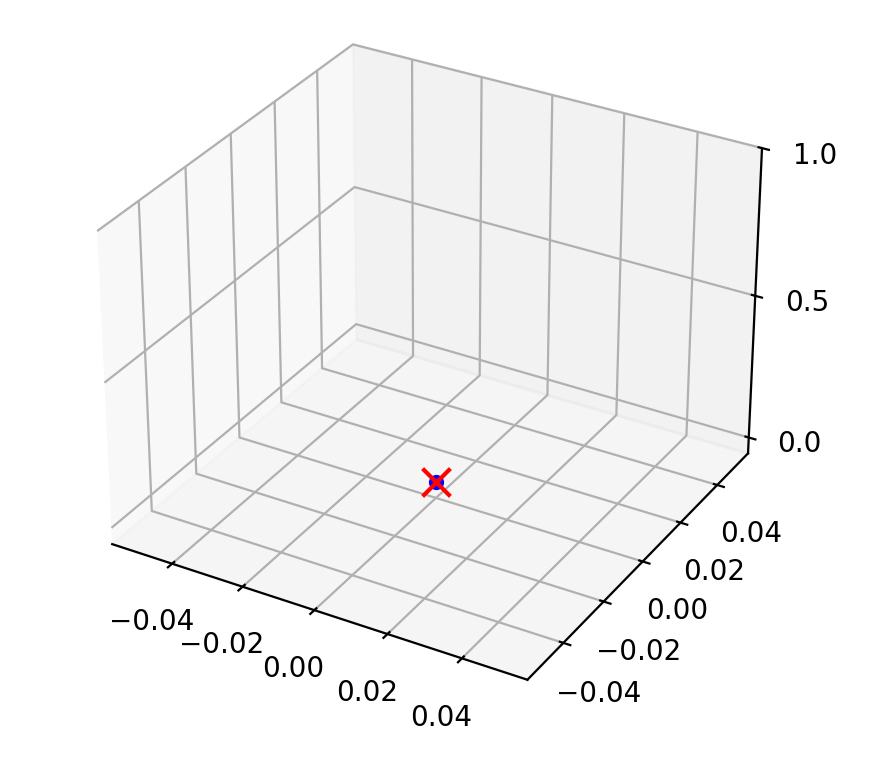
demo (a) \(n < d\): 1 sample, 2 features

\(X\)

\(X^\top\)

\(=\)

\(\begin{bmatrix}2\\3\end{bmatrix}\)

\(\begin{bmatrix}2 & 3\end{bmatrix}\)

\(= \begin{bmatrix}4 & 6\\6 & 9\end{bmatrix}\)

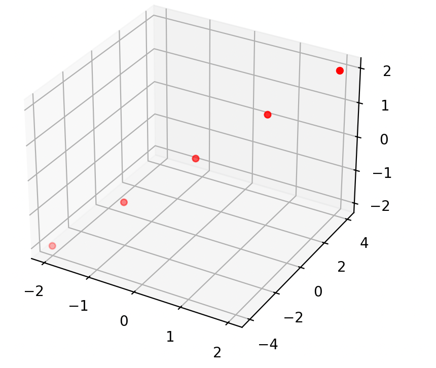
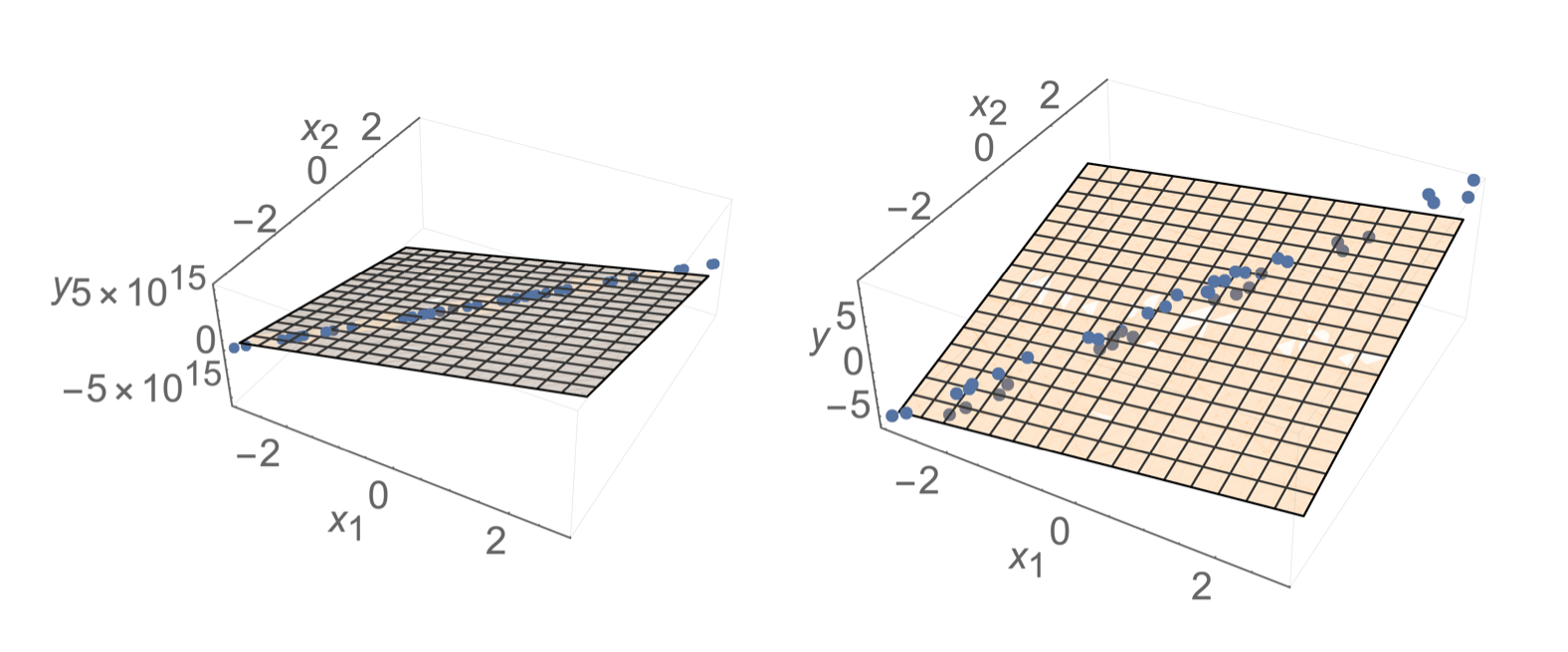
demo (b) Collinear: \(x_2 = 1.5 \cdot x_1\)

\(X\)

\(X^\top\)

\(=\)

\(\begin{bmatrix}2 & 4 & 6\\3 & 6 & 9\end{bmatrix}\)

\(\begin{bmatrix}2 & 3\\4 & 6\\6 & 9\end{bmatrix}\)

\(= \begin{bmatrix}56 & 84\\84 & 126\end{bmatrix}\)

mathematically,

This 👉 formula is not well-defined

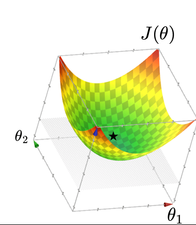
Typically, \(X\) is full column rank

\(\theta^*=\left({X}^{\top} {X}\right)^{-1} {X}^{\top} {Y}\)

\(J(\theta)\) "curves up" everywhere

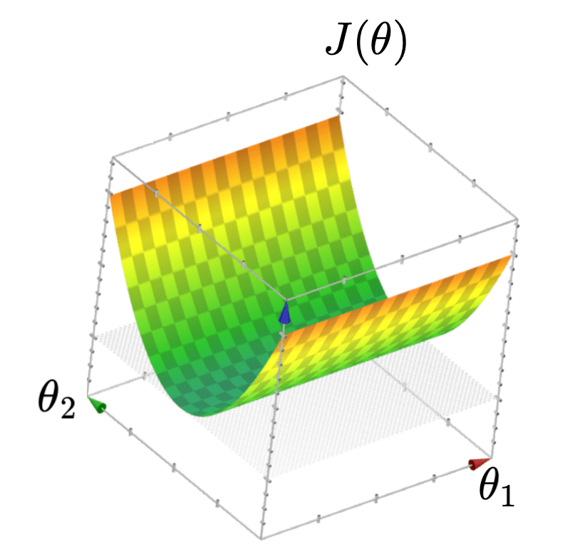
When \(X\) is not full column rank

\(J(\theta)\) has a "flat" bottom

Infinitely many optimal hyperplanes

unique optimal hyperplane

\(X^\top X\) is "more" invertible 🥰

formula isn't wrong, data is trouble-making 🥺

minimum eigenvalue of\((X^\top X)\) increasing

assume \(n=1\) and \(y=1\)

if the data is \((x,1) = (0.002,1)\)

if the data is \((x,y) = (-0.0002,1)\)

\(\theta^* = 500\)

\(\theta^* = -5,000\)

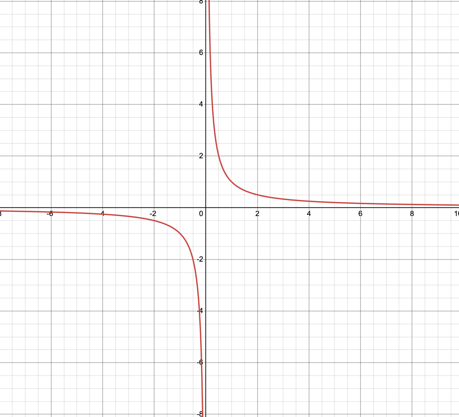
then \(\theta^*=\frac{1}{x}\)

technically, \(\theta^*=\left({X}^{\top} {X}\right)^{-1} {X}^{\top} {Y}\) exists and gives the unique optimal hyperplane

practically,

\(\theta^*\) tends to have huge magnitude

\(\theta^*\) tends to be very sensitive to the small changes in the data

when \(X^\top X\) is almost singular

lots of other \(\theta\)s fit the training data almost equally well

🥺

Outline

The "trouble" with the closed-form solution
Regularization and ridge regression
- hyperparameters
Cross-validation

Ridge Regression: Objective

Many \(\theta\) give similar loss, but some have huge magnitude... unstable!
- small change in \(x\) \(\Rightarrow\) wildly different prediction
Idea: penalize large \(\theta\) in our objective, a.k.a. (explicit) regularization
Ridge objective:

J_{\text{ridge}}(\theta)=\frac{1}{n}({X} \theta-{Y})^{\top}({X} \theta-{Y})+\lambda\|\theta\|^2

\phantom{J_{\text{ridge}}(\theta)=}\underbrace{\phantom{\frac{1}{n}({X} \theta-{Y})^{\top}({X} \theta-{Y})}}_{\substack{\text{MSE} \\ \text{(on training data)}}}

\phantom{J_{\text{ridge}}(\theta)=\frac{1}{n}({X} \theta-{Y})^{\top}({X} \theta-{Y})+}\underbrace{\phantom{\lambda\|\theta\|^2}}_{\substack{\text{penalty} \\ \text{(on parameter magnitude)}}}

\(\lambda > 0\) controls how heavily we penalize magnitude relative to MSE

Ridge Regression: Solution

J_{\text{ridge}}(\theta)=\frac{1}{n}({X} \theta-{Y})^{\top}({X} \theta-{Y})+\lambda\|\theta\|^2

for \(\lambda > 0\): \(\;{X}^{\top} {X}+n \lambda I\) is always invertible, so \(\theta^*_{\text{ridge}}\) always exists and is unique

How does \(\lambda\) affect the learned \(\theta\)?

\(\lambda = 0\)?
\(\lambda = 1000\)?
\(\lambda = -100\)?

No penalty — reduces to OLS
Huge penalty — forces \(\theta \approx 0\)
Rewards large \(\theta\) — counter-productive!

this is why we require \(\lambda > 0\)

\(\theta^*_{\text{ridge}}=\left({X}^{\top} {X}+n \lambda I\right)^{-1} {X}^{\top} {Y}\)

\boxed{h}

Regression

Algorithm

💻

\rightarrow

\downarrow

g

x

\downarrow

\(\in \mathbb{R}^d \)

\(\in \mathbb{R}\)

\(\mathcal{D}_\text{train}\)

\rightarrow

🧠 ⚙️

hypothesis class
loss function
hyperparameter

\(\lambda\) is a hyperparameter

affects learning outcome, and not learned by the algorithm
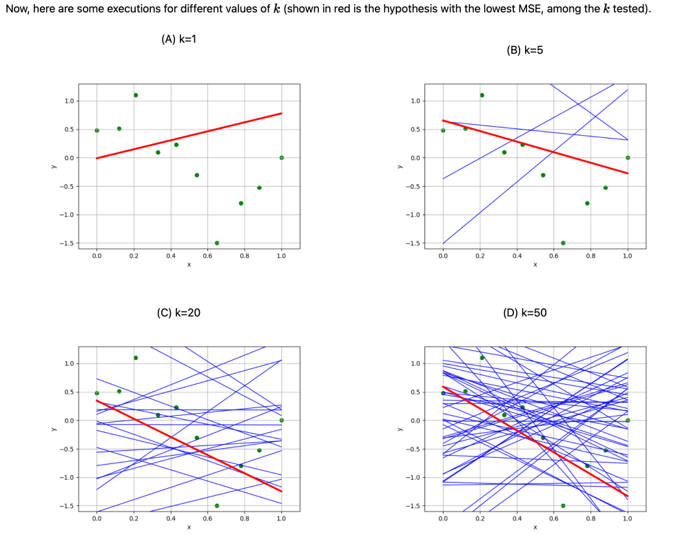
we already saw a hyperparameter (in lab 1, how many random regressor tried)

Outline

The "trouble" with the closed-form solution
Regularization and ridge regression
Cross-validation

We need to choose hyperparameters (like \(\lambda\))

Can’t use training error (would always pick \(\lambda=0\))
Can’t use test error (we don't have test data)

\(\left\{\left(x^{(1)}, y^{(1)}\right), \dots, \left(x^{(n)}, y^{(n)}\right)\right\}\)

\(\mathcal{D}_\text{val}\)

\(\mathcal{D}_\text{train}\)

Hold-out some data

Use \(\mathcal{D}_{\text{val}}\) to evaluate how good a hyperparameter \(\lambda\) is

\boxed{h_{\lambda}}

Regression

Algorithm

💻

\rightarrow

\downarrow

\rightarrow

🧠 ⚙️

linear hypothesis
ridge objective
a fixed \(\lambda\)

\mathcal{E}_{\text{val}}(\lambda)

train on \(\mathcal{D}_{\text{train}}\) with \(\lambda\)

compute \(\mathcal{E}_{\text{val}}(\lambda)\) on \(\mathcal{D}_{\text{val}}\)

for each \(\lambda \in \{0.1,\, 1,\, 10\}\):

train on \(\mathcal{D}_{\text{train}}\) with \(\lambda\)

compute \(\mathcal{E}_{\text{val}}(\lambda)\) on \(\mathcal{D}_{\text{val}}\)

return \(\arg\min_\lambda \mathcal{E}_{\text{val}}(\lambda)\)

\(\mathcal{D}_\text{val}\)

\(\mathcal{D}_\text{train}\)

in this example, compare \( \mathcal{E}_{\text{val}}(.1), \) \( \mathcal{E}_{\text{val}}(1), \) and \( \mathcal{E}_{\text{val}}(10), \)

return the \(\lambda\) corresponding to smallest validation error

Cross-validation

for \(i = 1, \dots, 5\):

train \(h_i\) on \(\mathcal{D} \setminus \mathcal{D}_i\) with \(\lambda\)

\(\mathcal{E}_i =\) error on \(\mathcal{D}_i\)

for \(i = 1, \dots, 5\):

train \(h_i\) on \(\mathcal{D} \setminus \mathcal{D}_i\) with \(\lambda\)

\(\mathcal{E}_i =\) error on \(\mathcal{D}_i\)

\(\mathcal{E}_{\text{val}}(\lambda) = (\mathcal{E}_1 + \cdots + \mathcal{E}_5) / 5\)

for each \(\lambda \in \{0.1, 1, 10\}\):

for \(i = 1, \dots, 5\):

train \(h_i\) on \(\mathcal{D} \setminus \mathcal{D}_i\) with \(\lambda\)

\(\mathcal{E}_i =\) error on \(\mathcal{D}_i\)

\(\mathcal{E}_{\text{val}}(\lambda) = (\mathcal{E}_1 + \cdots + \mathcal{E}_5) / 5\)

return \(\lambda^* = \arg\min_\lambda\,\mathcal{E}_{\text{val}}(\lambda)\)

for each \(\lambda \in \{0.1, 1, 10\}\):

for \(i = 1, \dots, 5\):

train \(h_i\) on \(\mathcal{D} \setminus \mathcal{D}_i\) with \(\lambda\)

\(\mathcal{E}_i =\) error on \(\mathcal{D}_i\)

\(\mathcal{E}_{\text{val}}(\lambda) = (\mathcal{E}_1 + \cdots + \mathcal{E}_5) / 5\)

return \(\lambda^* = \arg\min_\lambda\,\mathcal{E}_{\text{val}}(\lambda)\)

outer loop of \(\lambda \in \{0.1, 1, 10\}\):

\(\mathcal{E}_{\text{val}}(\lambda) = (\mathcal{E}_1 + \mathcal{E}_2 + \mathcal{E}_3 + \mathcal{E}_4 + \mathcal{E}_5) / 5\)

How many hypotheses trained in this example to pick \(\lambda^*\)?

\(\theta^*_{\text{final}} = (X^\top X + n \lambda^* I)^{-1} X^\top Y\)

finally train using the chosen \(\lambda^*,\) and data from all of \(\mathcal{D}\)

Two Ways X Can Fail

When is X not full column rank?

(a) \(n < d\) (more features than data points)	[common]
(b) linearly dependent features	[very common]

Common theme: not enough information to pin down a unique solution

flat MSE surface (like a half-pipe or valley)
infinitely many optimal \(\theta\)
\(\theta^* = (X^\top X)^{-1} X^\top Y\) is undefined

Let's visualize each...

\(\left({X}^{\top} {X}\right)\) is singular

\({X}\) is not full column rank

\(\left({X}^{\top} {X}\right)\) has zero eigenvalue(s)

\(\left({X}^{\top} {X}\right)\) is not full rank

the determinant of \(\left({X}^{\top} {X}\right)\) is zero

\Leftrightarrow

\(\theta^*=\left({X}^{\top} {X}\right)^{-1} {X}^{\top} {Y}\)

\(d\geq1\)

more generally,

most of the time, behaves nicely

but run into trouble when

The Problem with Validation

Validation error depends on luck of the split!

Same data, different random splits:

Split A: validation error = 0.15
Split B: validation error = 0.23

Which \(\lambda\) is actually best?

Cross-validation: average over ALL possible splits

Uses all data efficiently
More stable than single split
Gives reliable estimate of generalization
Uses all data for both training AND validation (just not at same time)

Cross-validation

for each \(\lambda \in \{0.1, 1, 10\}\):

for \(i = 1, \dots, 5\):

train \(h_i\) on \(\mathcal{D} \setminus \mathcal{D}_i\) with \(\lambda\)

\(\mathcal{E}_i =\) error on \(\mathcal{D}_i\)

\(\mathcal{E}_{\text{val}}(\lambda) = (\mathcal{E}_1 + \cdots + \mathcal{E}_5) / 5\)

return \(\lambda^* = \arg\min_\lambda\,\mathcal{E}_{\text{val}}(\lambda)\)

for each \(\lambda \in \{0.1, 1, 10\}\):

for \(i = 1, \dots, 5\):

train \(h_i\) on \(\mathcal{D} \setminus \mathcal{D}_i\) with \(\lambda\)

\(\mathcal{E}_i =\) error on \(\mathcal{D}_i\)

\(\mathcal{E}_{\text{val}}(\lambda) = (\mathcal{E}_1 + \cdots + \mathcal{E}_5) / 5\)

return \(\lambda^* = \arg\min_\lambda\,\mathcal{E}_{\text{val}}(\lambda)\)

for each \(\lambda \in \{0.1, 1, 10\}\):

for \(i = 1, \dots, 5\):

train \(h_i\) on \(\mathcal{D} \setminus \mathcal{D}_i\) with \(\lambda\)

\(\mathcal{E}_i =\) error on \(\mathcal{D}_i\)

\(\mathcal{E}_{\text{val}}(\lambda) = (\mathcal{E}_1 + \cdots + \mathcal{E}_5) / 5\)

return \(\lambda^* = \arg\min_\lambda\,\mathcal{E}_{\text{val}}(\lambda)\)

for each \(\lambda \in \{0.1, 1, 10\}\):

for \(i = 1, \dots, 5\):

train \(h_i\) on \(\mathcal{D} \setminus \mathcal{D}_i\) with \(\lambda\)

\(\mathcal{E}_i =\) error on \(\mathcal{D}_i\)

\(\mathcal{E}_{\text{val}}(\lambda) = (\mathcal{E}_1 + \cdots + \mathcal{E}_5) / 5\)

return \(\lambda^* = \arg\min_\lambda\,\mathcal{E}_{\text{val}}(\lambda)\)

How many hypotheses trained in this example to pick \(\lambda^*\)?

\(\theta^*_{\text{final}} = (X^\top X + n \lambda^* I)^{-1} X^\top Y\)

all of \(\mathcal{D}_1\) to \(\mathcal{D}_5\)

for \(\lambda \in \{0.1, 1, 10\}\):

Cross-validation

for \(i = 1, \dots, 5\):

train \(h_i\) on \(\mathcal{D} \setminus \mathcal{D}_i\) with \(\lambda\)

\(\mathcal{E}_i =\) error on \(\mathcal{D}_i\)

for \(i = 1, \dots, 5\):

train \(h_i\) on \(\mathcal{D} \setminus \mathcal{D}_i\) with \(\lambda\)

\(\mathcal{E}_i =\) error on \(\mathcal{D}_i\)

\(\mathcal{E}_{\text{val}}(\lambda) = (\mathcal{E}_1 + \cdots + \mathcal{E}_5) / 5\)

for each \(\lambda \in \{0.1, 1, 10\}\):

for \(i = 1, \dots, 5\):

train \(h_i\) on \(\mathcal{D} \setminus \mathcal{D}_i\) with \(\lambda\)

\(\mathcal{E}_i =\) error on \(\mathcal{D}_i\)

\(\mathcal{E}_{\text{val}}(\lambda) = (\mathcal{E}_1 + \cdots + \mathcal{E}_5) / 5\)

return \(\lambda^* = \arg\min_\lambda\,\mathcal{E}_{\text{val}}(\lambda)\)

for each \(\lambda \in \{0.1, 1, 10\}\):

for \(i = 1, \dots, 5\):

train \(h_i\) on \(\mathcal{D} \setminus \mathcal{D}_i\) with \(\lambda\)

\(\mathcal{E}_i =\) error on \(\mathcal{D}_i\)

\(\mathcal{E}_{\text{val}}(\lambda) = (\mathcal{E}_1 + \cdots + \mathcal{E}_5) / 5\)

return \(\lambda^* = \arg\min_\lambda\,\mathcal{E}_{\text{val}}(\lambda)\)

outer loop of \(\lambda \in \{0.1, 1, 10\}\):

\(\mathcal{E}_{\text{val}}(\lambda) = (\mathcal{E}_1 + \mathcal{E}_2 + \mathcal{E}_3 + \mathcal{E}_4 + \mathcal{E}_5) / 5\)

How many hypotheses trained in this example to pick \(\lambda^*\)?

\(\theta^*_{\text{final}} = (X^\top X + n \lambda^* I)^{-1} X^\top Y\)

finally train using data from all of \(\mathcal{D}\)

Lecture 2: Regularization and Cross-validation

Intro to Machine Learning

Outline

Outline

Outline

Summary