

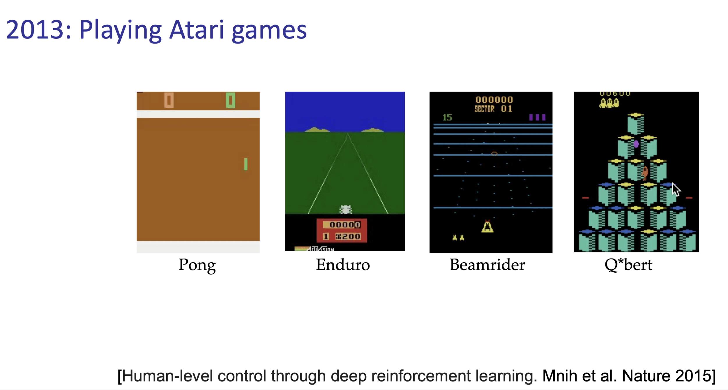
Lecture 10: Markov Decision Processes
Intro to Machine Learning

Toddler demo, Russ Tedrake thesis, 2004
uses vanilla policy gradient (actor-critic)


Reinforcement Learning with Human Feedback
Outline
- Markov Decision Processes Definition
-
Policy Evaluation
-
State value functions: \(\mathrm{V}^{\pi}\)
-
Bellman recursions and Bellman equations
-
-
Policy Optimization
-
Optimal policies \(\pi^*\)
-
Optimal action value functions: \(\mathrm{Q}^*\)
-
Value iteration
-
- Markov Decision Processes Definition
-
Policy Evaluation
-
State value functions: \(\mathrm{V}^{\pi}\)
-
Bellman recursions and Bellman equations
-
-
Policy Optimization
-
Optimal policies \(\pi^*\)
-
Optimal action value functions: \(\mathrm{Q}^*\)
-
Value iteration
-
Markov Decision Processes
-
Research area initiated in the 50s by Bellman, known under various names:
-
Stochastic optimal control (Control theory)
-
Stochastic shortest path (Operations research)
-
Sequential decision making under uncertainty (Economics)
-
Reinforcement learning (Artificial intelligence, Machine learning)
-
-
A rich variety of elegant theory, mathematics, algorithms, and applications, but also considerable variation in notation.
-
We will use the most RL-flavored notations.
- (state, action) results in a transition \(\mathrm{T}\) into a next state:
-
Normally, we get to the “intended” state;
-
E.g., in state (7), action “↑” gets to state (4)
-
-
If an action would take Mario out of the grid world, stay put;
-
E.g., in state (9), “→” gets back to state (9)
-
-
In state (6), action “↑” leads to two possibilities:
-
20% chance to (2)
-
80% chance to (3).
-
-
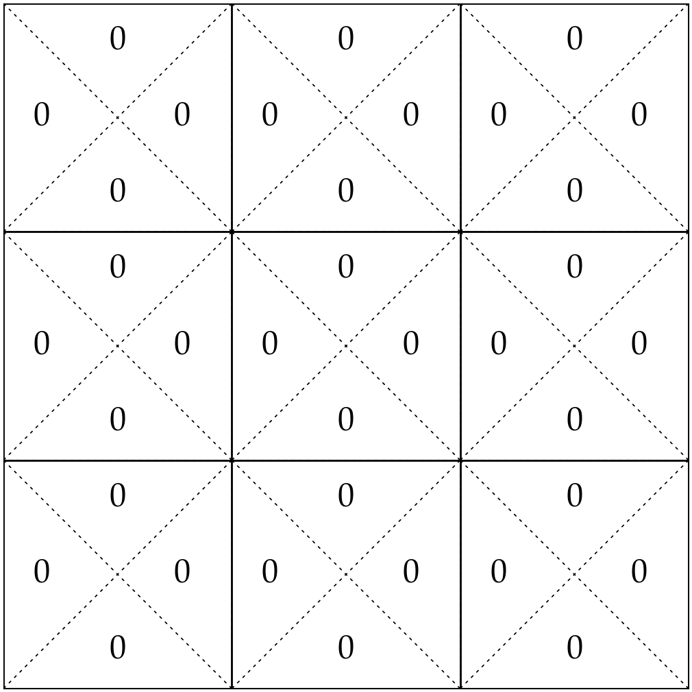
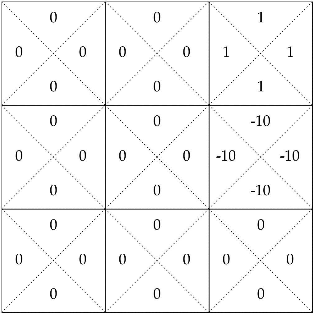
Running example: Mario in a grid-world

- 9 possible states \(s\)
- 4 possible actions \(a\): {Up ↑, Down ↓, Left ←, Right →}

reward of (3, \(\downarrow\))
reward of \((3,\uparrow\))
reward of \((6, \downarrow\))
reward of \((6,\rightarrow\))
- (state, action) pairs give rewards:
- in state 3, any action gives reward 1
- in state 6, any action gives reward -10
- any other (state, action) pair gives reward 0

-
discount factor: a scalar of 0.9 that reduces the 'worth' of future rewards depending on when Mario receives them.
- So, e.g., for (3, \(\leftarrow\)) pair, Mario gets
- at the start of the game, a reward of 1
- at the 2nd time step, a discounted reward of 0.9
- at the 3rd time step, a further discounted reward of \((0.9)^2\) ... and so on
- So, e.g., for (3, \(\leftarrow\)) pair, Mario gets


Mario in a grid-world, cont'd

- \(\mathcal{S}\) : state space, contains all possible states \(s\).
- \(\mathcal{A}\) : action space, contains all possible actions \(a\).
- \(\mathrm{T}\left(s, a, s^{\prime}\right)\) : the probability of transition from state \(s\) to \(s^{\prime}\) when action \(a\) is taken.
Markov Decision Processes - Definition and terminologies
\(\mathrm{T}\left(7, \uparrow, 4\right) = 1\)
\(\mathrm{T}\left(9, \rightarrow, 9\right) = 1\)
\(\mathrm{T}\left(6, \uparrow, 3\right) = 0.8\)
\(\mathrm{T}\left(6, \uparrow, 2\right) = 0.2\)
In 6.390,
- \(\mathcal{S}\) and \(\mathcal{A}\) are small discrete sets, unless otherwise specified.
- \(s^{\prime}\) and \(a^{\prime}\) are short-hand for the next-timestep state and action.

- \(\mathcal{S}\) : state space, contains all possible states \(s\).
- \(\mathcal{A}\) : action space, contains all possible actions \(a\).
- \(\mathrm{T}\left(s, a, s^{\prime}\right)\) : the probability of transition from state \(s\) to \(s^{\prime}\) when action \(a\) is taken.
- \(\mathrm{R}(s, a)\) : reward, takes in a (state, action) pair and returns a reward.
Markov Decision Processes - Definition and terminologies
reward of \((3,\uparrow\))
reward of \((6,\rightarrow\))
\(\mathrm{R}\left(3, \uparrow \right) = 1\)
\(\mathrm{R}\left(6, \rightarrow \right) = -10\)
In 6.390,
- \(\mathcal{S}\) and \(\mathcal{A}\) are small discrete sets, unless otherwise specified.
- \(s^{\prime}\) and \(a^{\prime}\) are short-hand for the next-timestep state and action.
- \(\mathrm{R}(s, a)\) is deterministic and bounded.
- \(\mathcal{S}\) : state space, contains all possible states \(s\).
- \(\mathcal{A}\) : action space, contains all possible actions \(a\).
- \(\mathrm{T}\left(s, a, s^{\prime}\right)\) : the probability of transition from state \(s\) to \(s^{\prime}\) when action \(a\) is taken.
- \(\mathrm{R}(s, a)\) : reward, takes in a (state, action) pair and returns a reward.
- \(\gamma \in [0,1]\): discount factor, a scalar.
- \(\pi{(s)}\) : policy, takes in a state and returns an action.
The goal of an MDP is to find a good policy.
Markov Decision Processes - Definition and terminologies
In 6.390,
- \(\mathcal{S}\) and \(\mathcal{A}\) are small discrete sets, unless otherwise specified.
- \(s^{\prime}\) and \(a^{\prime}\) are short-hand for the next-timestep state and action.
- \(\mathrm{R}(s, a)\) is deterministic and bounded.
- \(\pi(s)\) is deterministic.
- \(a_t = \pi(s_t)\)
- \(r_t = \mathrm{R}(s_t,a_t)\)
Policy \(\pi(s)\)
Transition \(\mathrm{T}\left(s, a, s^{\prime}\right)\)
Reward \(\mathrm{R}(s, a)\)
time
a trajectory (also called an experience or rollout) of horizon \(h\)
\(\quad \tau=\left(s_0, a_0, r_0, s_1, a_1, r_1, \ldots s_{h-1}, a_{h-1}, r_{h-1}\right)\)
initial state
all depends on \(\pi\)
- \(\mathrm{T}\left(s, a, s^{\prime}\right)\)
Outline
- Markov Decision Processes Definition
-
Policy Evaluation
-
State value functions: \(\mathrm{V}^{\pi}\)
-
Bellman recursions and Bellman equations
-
-
Policy Optimization
-
Optimal policies \(\pi^*\)
-
Optimal action value functions: \(\mathrm{Q}^*\)
-
Value iteration
-
Starting in state \(s\), how good is it to follow a given policy \(\pi\) for \(h\) time steps?
One idea:
But if we start at \(s_0=6\) and follow the "always-up" policy:
👈
states and one special transition:
rewards:
trajectory:

Reward \(\mathrm{R}(s, a)\)
Policy \(\pi(s)\)
Transition \(\mathrm{T}\left(s, a, s^{\prime}\right)\)
time
Value functions:
- \(\mathrm{V}_h^\pi(s):\) expected sum of discounted rewards starting in state \(s\) and follow \(\pi\) for \(h\) steps
- Value is long-term; reward is immediate (one-time)
- Convention: \(\mathrm{V}_0^\pi(s)=0\) for all states
- The value expectation in 6.390 is only w.r.t. the transition probabilities \(\mathrm{T}\left(s, a, s^{\prime}\right)\)
(eq. 1️⃣)
\( h\) terms
evaluate \(\mathrm{V}_h^\pi(s)\) under the "always-up" policy
states and
one special transition:
rewards
- \(\pi(s) = ``\uparrow",\ \forall s\)
- \(\gamma = 0.9\)
horizon \(h\) = 0: no step left

horizon \(h\) = 1: receive the rewards
horizon \(h = 2\)
states and
one special transition:
rewards
- \(\pi(s) = ``\uparrow",\ \forall s\)
- \(\gamma = 0.9\)
\( 2\) terms
action \(\uparrow\)


action \(\uparrow\)
action \(\uparrow\)
horizon \(h = 2\)
states and
one special transition:
rewards
- \(\pi(s) = ``\uparrow",\ \forall s\)
- \(\gamma = 0.9\)
\( 2\) terms
action \(\uparrow\)
action \(\uparrow\)
action \(\uparrow\)
action \(\uparrow\)
action \(\uparrow\)
states and
one special transition:
rewards
- \(\pi(s) = ``\uparrow",\ \forall s\)
- \(\gamma = 0.9\)
horizon \(h = 3\)
\( 3\) terms
the immediate reward for taking the policy-prescribed action \(\pi(s)\) in state \(s\).
horizon-\(h\) value in state \(s\): the expected sum of discounted rewards, starting in state \(s\) and following policy \(\pi\) for \(h\) steps.
\((h-1)\) horizon future value at a next state \(s^{\prime}\)
sum of future values weighted by the probability of reaching that next state \(s^{\prime}\)
discounted by \(\gamma\)
(eq. 2️⃣)
Bellman Recursion (eq. 2️⃣)
states and
one special transition:
rewards
- \(\pi(s) = ``\uparrow",\ \forall s\)
- \(\gamma = 0.9\)
states and
one special transition:
rewards
- \(\pi(s) = ``\uparrow",\ \forall s\)
- \(\gamma = 0.9\)
Bellman Recursion (eq. 2️⃣)
states and
one special transition:
rewards
- \(\pi(s) = ``\uparrow",\ \forall s\)
- \(\gamma = 0.9\)
Bellman Recursion (eq. 2️⃣)

states and
one special transition:
rewards
- \(\pi(s) = ``\uparrow",\ \forall s\)
- \(\gamma = 0.9\)
Bellman Recursion (eq. 2️⃣)
states and
one special transition:
rewards
- \(\pi(s) = ``\uparrow",\ \forall s\)
- \(\gamma = 0.9\)
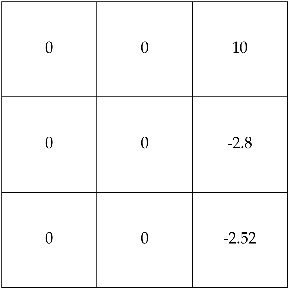
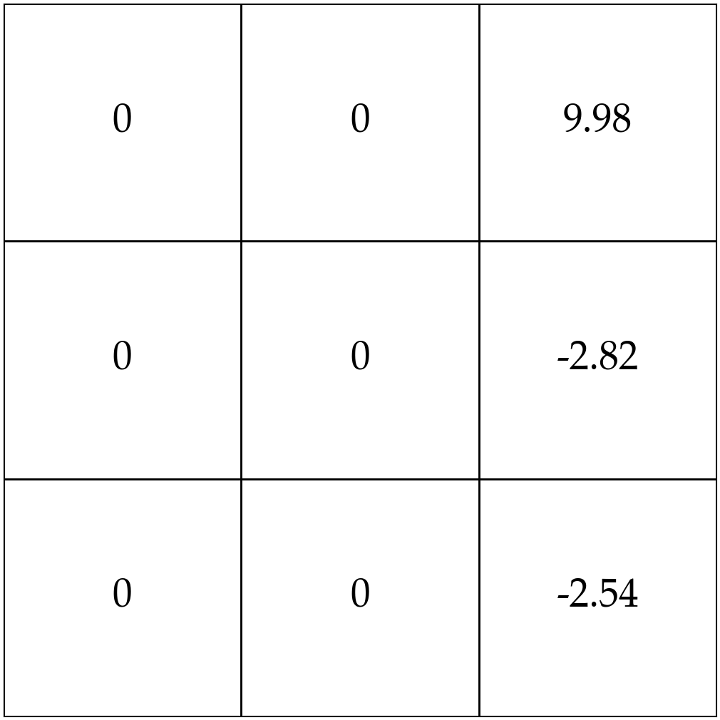
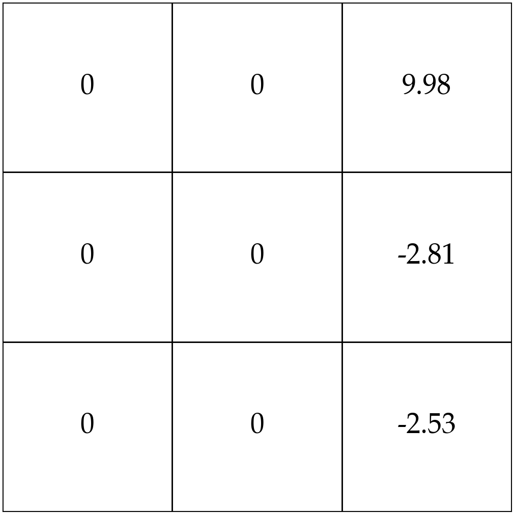
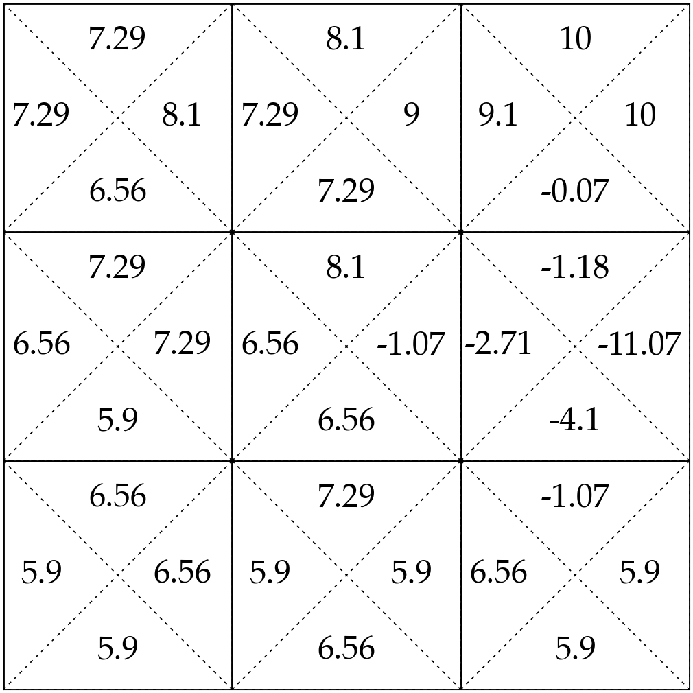
- As we extend the horizon, value differences shrink
- because longer-term rewards are heavily discounted
- so, as \(h \to \infty,\) the value functions stop changing
- convergence can be seen, e.g., via \(\mathrm{V}^{\uparrow}_{\infty}(3)=1+.9+.9^2+.9^3 + \dots =10\)
Value functions converge as \(h \to \infty\)
Typically, \(\gamma < 1\) to ensure \(\mathrm{V}_{\infty}\) is finite.
states and
one special transition:
rewards
- \(\pi(s) = ``\uparrow",\ \forall s\)
- \(\gamma = 0.9\)
Recursion (finite \(h\)) 2️⃣
As horizon \(h \to \infty,\) the Bellman recursion becomes the Bellman equation
Equation \((h\to \infty)\) 3️⃣
A system of \(|\mathcal{S}|\) self-consistent linear equations, one for each state
finite-horizon Bellman recursions
infinite-horizon Bellman equations
Policy Evaluation
Quick summary
Use the definition and sum up expected rewards:
Or, leverage the recursive structure:
1️⃣
2️⃣
3️⃣
Outline
- Markov Decision Processes Definition
-
Policy Evaluation
-
State value functions: \(\mathrm{V}^{\pi}\)
-
Bellman recursions and Bellman equations
-
-
Policy Optimization
-
Optimal policies \(\pi^*\)
-
Optimal action value functions: \(\mathrm{Q}^*\)
-
Value iteration
-
- Intuitively, an optimal policy \(\pi^*\) is a policy that yields the highest possible value \(\mathrm{V}_h^{*}({s})\) from every state
- An MDP in 6.390 has a unique optimal value \(\mathrm{V}_h^{*}({s})\)
- Optimal policy \(\pi^*\) might not be unique
Optimal policy \(\pi^*\)
e.g. in the "Luigi game", any policy is an optimal policy
\(\gamma = 0.9\)
States and one special transition:
Rewards:

- Formally: an optimal policy \(\pi^*\) is such that: \[\mathrm{V}_h^{\pi^*}(s) = \max_{\pi} \mathrm{V}_h^{\pi}(s) = \mathrm{V}_h^*(s), \forall s \in \mathcal{S}\]
- How to search for an optimal policy \(\pi^*\)?
- Even if we tediously enumerate over all \(\pi\), do policy evaluation, compare values to get \(\mathrm{V}^{*}_h(s)\)...it's not yet clear how to choose actions.
\(\mathrm{V}^*(s)\) is defined over states, not actions.
It tells us where we'd like to be — not what we should do to get there.
Optimal policy \(\pi^*\)
\(\mathrm{V}_h^*(s) = \max_{a} \big[\mathrm{R}(s, a) + \gamma \sum_{s'} \mathrm{T}(s, a, s') \mathrm{V}_{h-1}^*(s') \big]\)
Policy \(\pi(s)\)
Transition \(\mathrm{T}\left(s, a, s^{\prime}\right)\)
Reward \(\mathrm{R}(s, a)\)
time
if we've acted optimally for \(h\) steps: \(\mathrm{V}_h^*(s)\)
we must have acted optimally from the first step onward \(\mathrm{V}_{h-1}^*(s')\)
(new, eq. 4️⃣, for an optimal policy)
(recall, eq. 2️⃣, for any policy)
with the first step action
that led to the optimal future
Define the optimal state-action value functions \(\mathrm{Q}^*_h(s, a):\)
the expected sum of discounted rewards, obtained by
- starting in state \(s\)
- take action \(a\), for one step
- act optimally thereafter for the remaining \((h-1)\) steps
\(\mathrm{Q}^*\) satisfies:
\[\mathrm{Q}^*_h (s, a)=\mathrm{R}(s, a)+\gamma \sum_{s^{\prime}} \mathrm{T}\left(s, a, s^{\prime} \right) \max _{a^{\prime}} \mathrm{Q}^*_{h-1}\left(s^{\prime}, a^{\prime}\right)\]
(eq. 5️⃣)
\(\mathrm{Q}^*_{h}(s, a)\)
(eq. 4️⃣)
\(\mathrm{V}_h^*(s) = \max_{a} \big[\mathrm{R}(s, a) + \gamma \sum_{s'} \mathrm{T}(s, a, s') \mathrm{V}_{h-1}^*(s') \big]\)
- starting in state \(s\),
- take action \(a\), for one step
- act optimally thereafter for the remaining \((h-1)\) steps
\(\mathrm{Q}^*_h(s, a)\): the value for
\(\gamma = 0.9\)
States and one special transition:
Rewards:
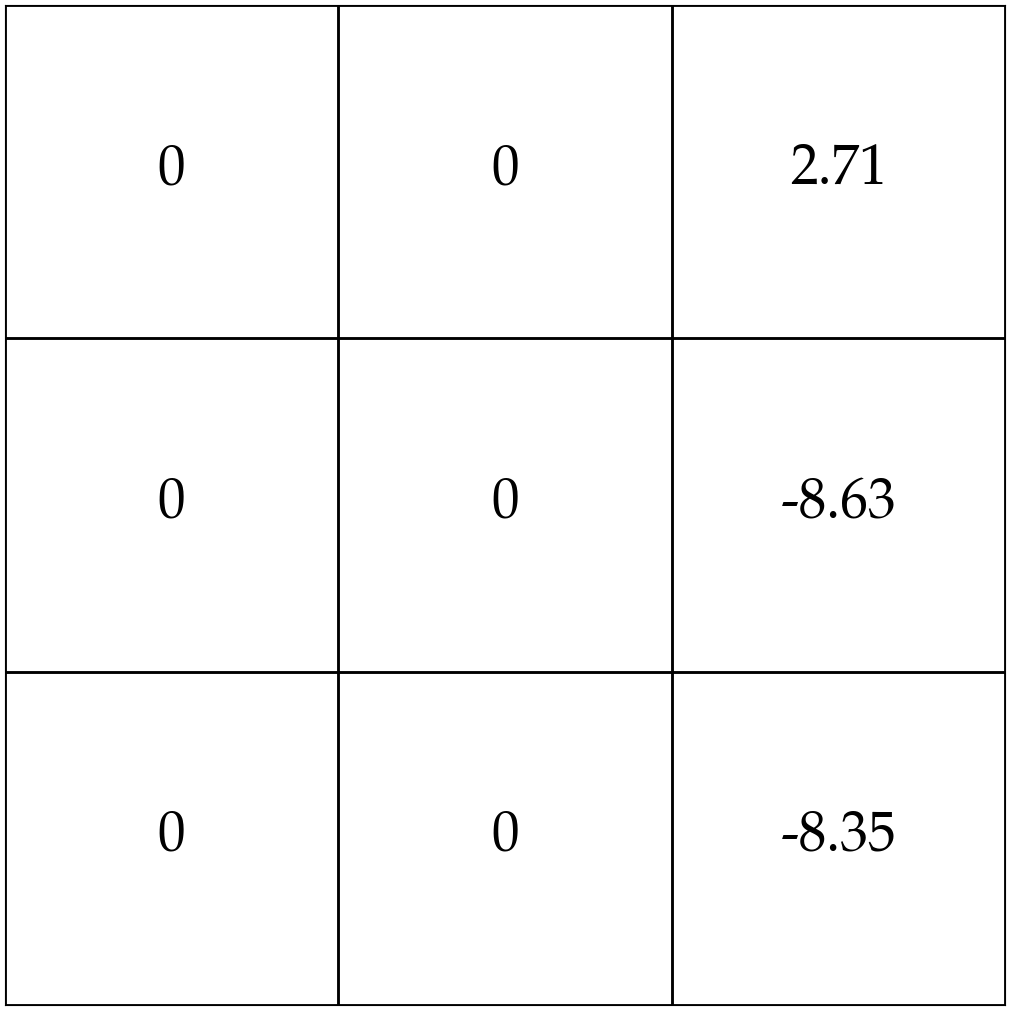
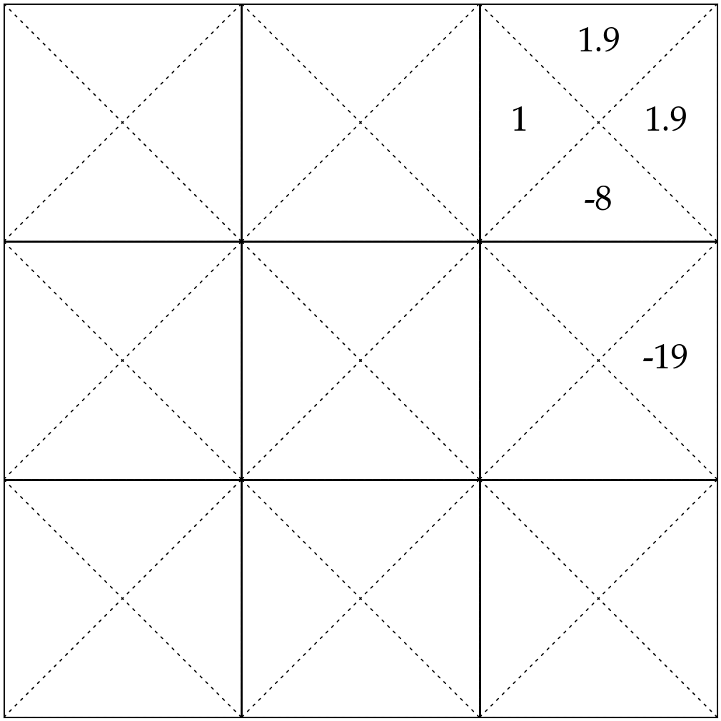
Consider \(\mathrm{Q}^*_2(3, \downarrow)\)
- receive \(\mathrm{R}(3,\downarrow)\)
\( = 1 + .9\times -10\)
- next state \(s'\) = 6, act optimally for the remaining one timestep
- receive \(\max _{a^{\prime}} \mathrm{Q}_{1}^*\left(6, a^{\prime}\right)\)
\( = -8\)
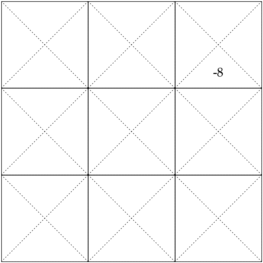
\(\mathrm{Q}_2^*(3, \downarrow) = \mathrm{R}(3,\downarrow) + \gamma \max _{a^{\prime}} \mathrm{Q}_{1}^*\left(6, a^{\prime}\right)\)
- starting in state \(s\),
- take action \(a\), for one step
- act optimally thereafter for the remaining \((h-1)\) steps
\(\mathrm{Q}^*_h(s, a)\): the value for
\(\gamma = 0.9\)
States and one special transition:
Rewards:
Let's consider \(\mathrm{Q}_2^*(3, \leftarrow)\)
- receive \(\mathrm{R}(3,\leftarrow)\)
\( = 1 + .9\times0 \)
- next state \(s'\) = 2, act optimally for the remaining one timestep
- receive \(\max _{a^{\prime}} \mathrm{Q}_{1}^*\left(2, a^{\prime}\right)\)
\( = 1\)
\(\mathrm{Q}_2^*(3, \leftarrow) = \mathrm{R}(3,\leftarrow) + \gamma \max _{a^{\prime}} \mathrm{Q}_{1}^*\left(2, a^{\prime}\right)\)
- starting in state \(s\),
- take action \(a\), for one step
- act optimally thereafter for the remaining \((h-1)\) steps
\(\mathrm{Q}^*_h(s, a)\): the value for
\(\gamma = 0.9\)
States and one special transition:
Rewards:
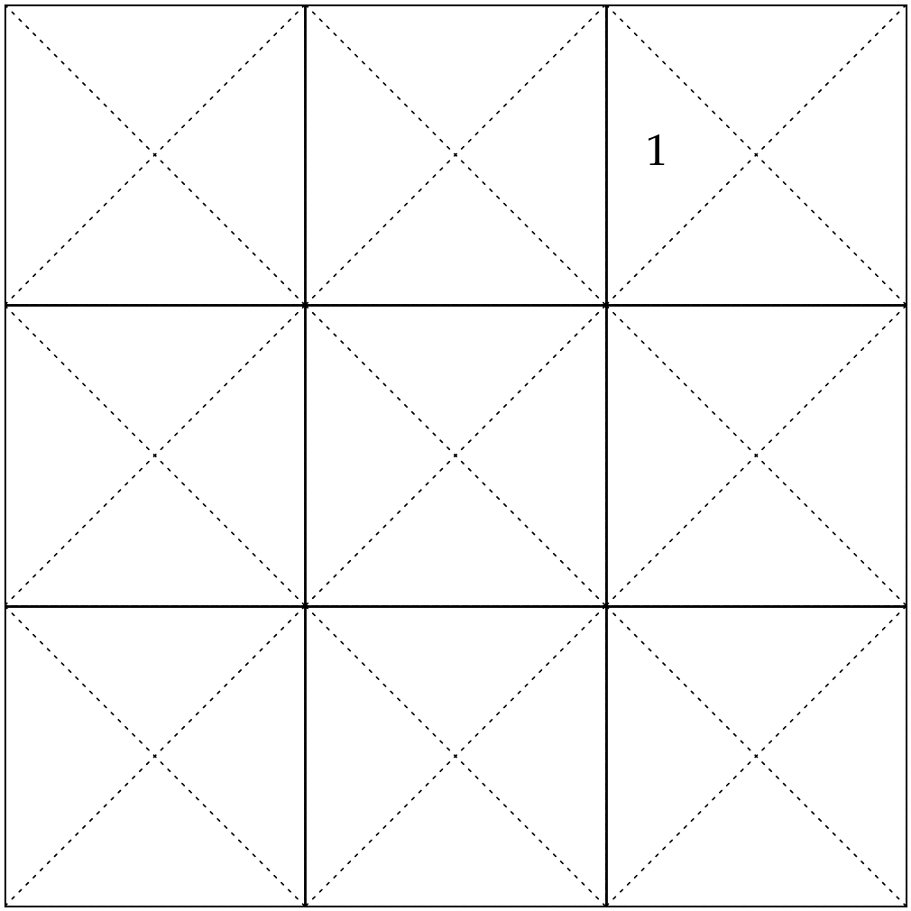
Let's consider \(\mathrm{Q}^*_2(3, \uparrow)\)
- receive \(\mathrm{R}(3,\uparrow)\)
\( = 1 + .9 \times 1\)
- next state \(s'\) = 3, act optimally for the remaining one timestep
- receive \(\max _{a^{\prime}} \mathrm{Q}^*_{1}\left(3, a^{\prime}\right)\)
\( = 1.9\)
\(\mathrm{Q}^*_2(3, \uparrow) = \mathrm{R}(3,\uparrow) + \gamma \max _{a^{\prime}} \mathrm{Q}^*_{1}\left(3, a^{\prime}\right)\)
- starting in state \(s\),
- take action \(a\), for one step
- act optimally thereafter for the remaining \((h-1)\) steps
\(\mathrm{Q}^*_h(s, a)\): the value for
\(\gamma = 0.9\)
States and one special transition:
Rewards:
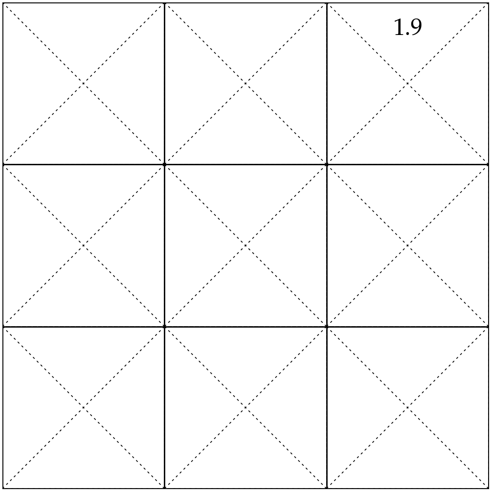
Let's consider \(\mathrm{Q}^*_2(3, \rightarrow)\)
- receive \(\mathrm{R}(3,\rightarrow)\)
\( = 1 + .9\times1\)
- next state \(s'\) = 3, act optimally for the remaining one timestep
- receive \(\max _{a^{\prime}} \mathrm{Q}^*_{1}\left(3, a^{\prime}\right)\)
\( = 1.9\)
\(\mathrm{Q}^*_2(3, \rightarrow) = \mathrm{R}(3,\rightarrow) + \gamma \max _{a^{\prime}} \mathrm{Q}^*_{1}\left(3, a^{\prime}\right)\)
- starting in state \(s\),
- take action \(a\), for one step
- act optimally thereafter for the remaining \((h-1)\) steps
\(\mathrm{Q}^*_h(s, a)\): the value for
\(\gamma = 0.9\)
States and one special transition:
Rewards:
- act optimally at the next state \(s^{\prime}=6\)
receive \(\max _{a^{\prime}} \mathrm{Q}_{1}^*\left(6, a^{\prime}\right)\)
- receive \(\mathrm{R}(6,\rightarrow)\)
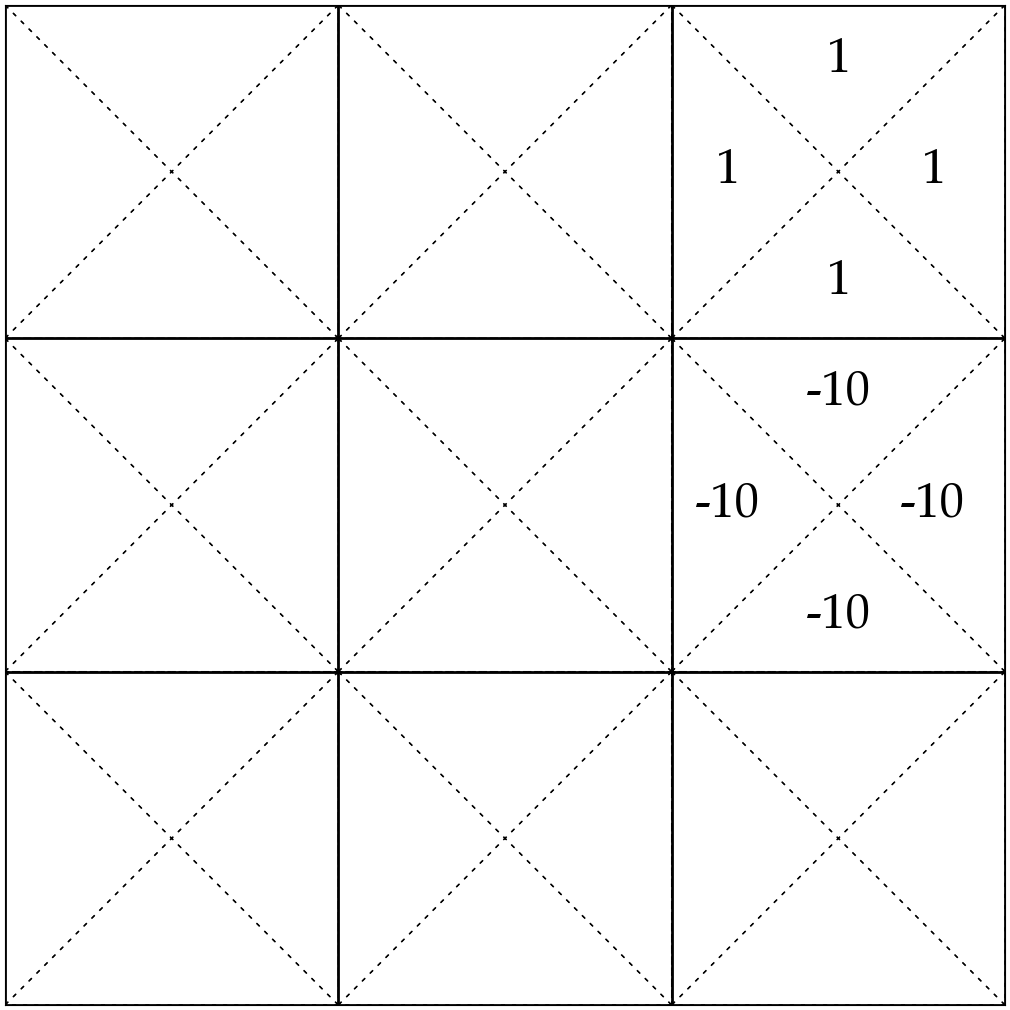
Let's consider \(\mathrm{Q}_2^*(6, \rightarrow) \)
\(\mathrm{Q}_2^*(6, \rightarrow)=\mathrm{R}(6,\rightarrow) + \gamma[\max _{a^{\prime}} \mathrm{Q}_{1}^*\left(6, a^{\prime}\right)] \)
\( = -10 + .9 \times -10 \Rightarrow -19\)
- starting in state \(s\),
- take action \(a\), for one step
- act optimally thereafter for the remaining \((h-1)\) steps
\(\mathrm{Q}^*_h(s, a)\): the value for
\(\gamma = 0.9\)
States and one special transition:
Rewards:

- act optimally at the next state \(s^{\prime}\)
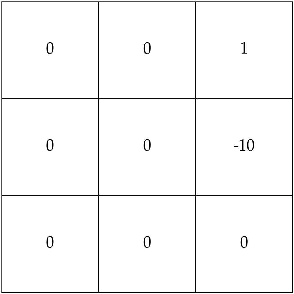
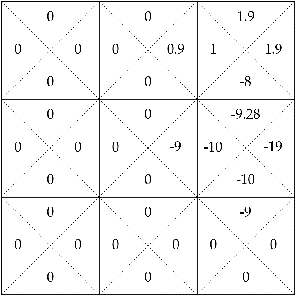
- 20% chance, \(s'\) = 2, act optimally, get \(\max _{a^{\prime}} \mathrm{Q}_{1}^*\left(2, a^{\prime}\right)\)
- 80% chance, \(s'\) = 3, act optimally, get \(\max _{a^{\prime}} \mathrm{Q}_{1}^*\left(3, a^{\prime}\right)\)
\(= -10 + .9 [.2 \times 0+ .8 \times 1] \Rightarrow -9.28\)
- receive \(\mathrm{R}(6,\uparrow)\)
Let's consider \(\mathrm{Q}_2^*(6, \uparrow) \)
\(\mathrm{Q}_2^*(6, \uparrow)=\mathrm{R}(6,\uparrow) + \gamma[.2 \max _{a^{\prime}} \mathrm{Q}_{1}^*\left(2, a^{\prime}\right)+ .8\max _{a^{\prime}} \mathrm{Q}_{1}^*\left(3, a^{\prime}\right)] \)
- starting in state \(s\),
- take action \(a\), for one step
- act optimally thereafter for the remaining \((h-1)\) steps
\(\mathrm{Q}^*_h(s, a)\): the value for
\(\gamma = 0.9\)
States and one special transition:
Rewards:
- starting in state \(s\),
- take action \(a\), for one step
- act optimally thereafter for the remaining \((h-1)\) steps
\(\mathrm{Q}^*_h(s, a)\): the value for
\(\gamma = 0.9\)
States and one special transition:
Rewards:
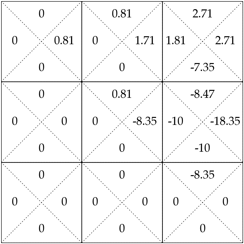
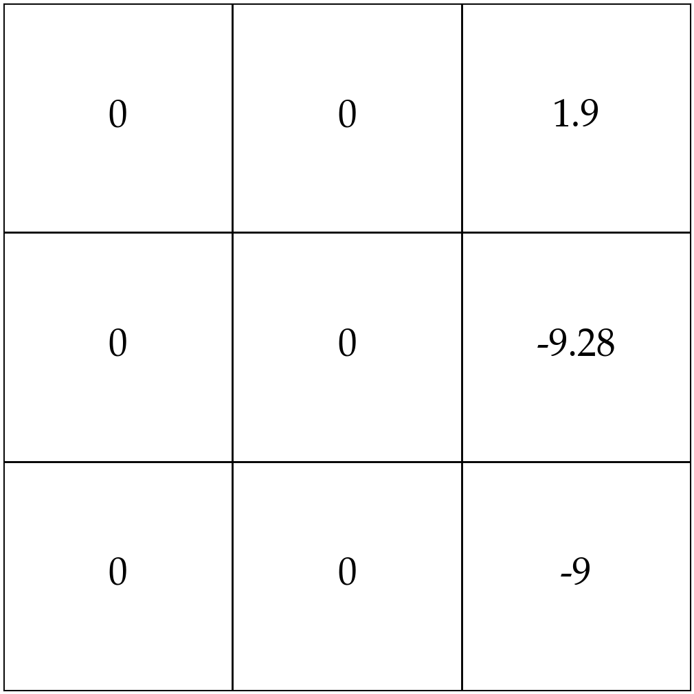
\(= -10 + .9 [.2 \times 0.9 + .8 \times 1.9] \Rightarrow -8.47\)
\(\mathrm{Q}_3^*(6, \uparrow)=\mathrm{R}(6,\uparrow) + \gamma[.2 \max _{a^{\prime}} \mathrm{Q}_{2}^*\left(2, a^{\prime}\right)+ .8\max _{a^{\prime}} \mathrm{Q}_{2}^*\left(3, a^{\prime}\right)] \)
Let's consider \(\mathrm{Q}_3^*(6, \uparrow) \)
- receive \(\mathrm{R}(6,\uparrow)\)
- 20% chance, \(s'\) = 2, act optimally, get \(\max _{a^{\prime}} \mathrm{Q}_{2}^*\left(2, a^{\prime}\right)\)
- act optimally at the next state \(s^{\prime}\)
- 80% chance, \(s'\) = 3, act optimally, get \(\max _{a^{\prime}} \mathrm{Q}_{2}^*\left(3, a^{\prime}\right)\)
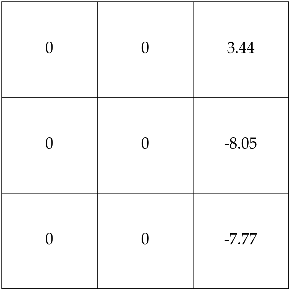
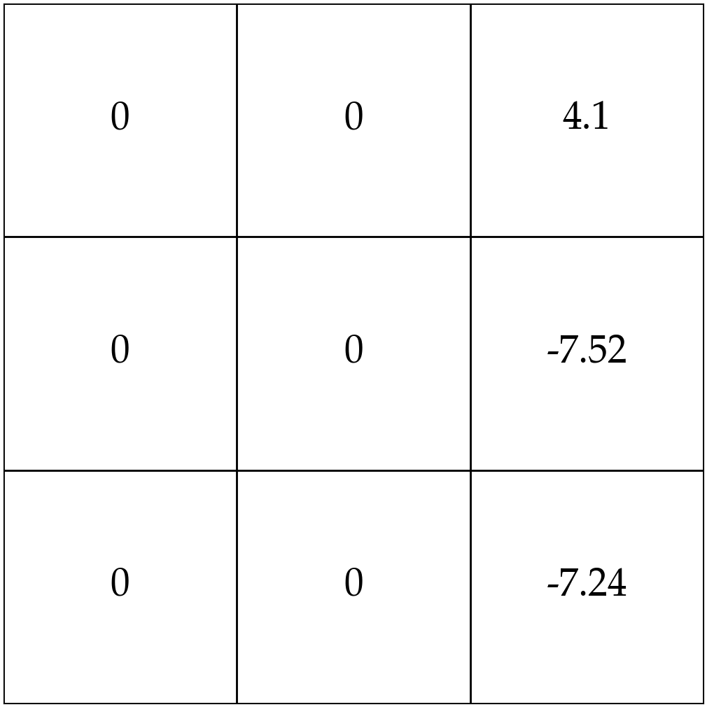
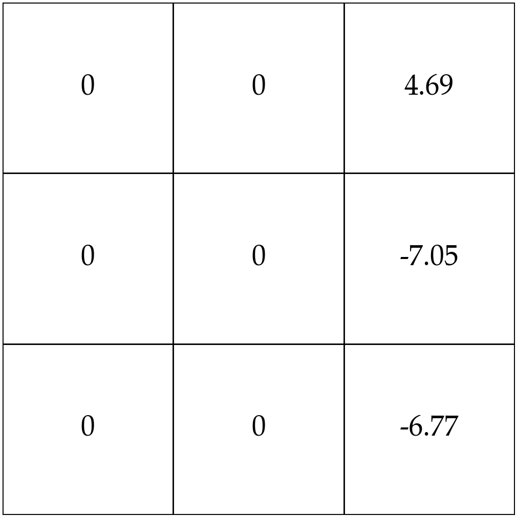
- for \(s \in \mathcal{S}, a \in \mathcal{A}\) :
- \(\mathrm{Q}_{\text {old }}(\mathrm{s}, \mathrm{a})=0\)
- while True:
- for \(s \in \mathcal{S}, a \in \mathcal{A}\) :
- \(\mathrm{Q}_{\text {new }}(s, a) \leftarrow \mathrm{R}(s, a)+\gamma \sum_{s^{\prime}} \mathrm{T}\left(s, a, s^{\prime}\right) \max _{a^{\prime}} \mathrm{Q}_{\text {old }}\left(s^{\prime}, a^{\prime}\right)\)
- if \(\max _{s, a}\left|Q_{\text {old }}(s, a)-Q_{\text {new }}(s, a)\right|<\epsilon:\)
- return \(\mathrm{Q}_{\text {new }}\)
- \(\mathrm{Q}_{\text {old }} \leftarrow \mathrm{Q}_{\text {new }}\)
Value Iteration
if run this block \(h\) times and break, then the returns are exactly \(\mathrm{Q}^*_h\)
\(\mathrm{Q}^*_{\infty}(s, a)\)
Value iteration: what we just did, iteratively invoke (eq. 5️⃣):
Optimal policy easily extracted: 6️⃣
e.g. the best actions to take in state 5
- For finite \(h\), optimal policy \(\pi^*_h\) depends on how many time steps are left
- When \(h \rightarrow \infty\), time no longer matters, i.e., there exists a stationary \(\pi^*\)
Summary
A Markov decision process \((\mathcal{S}, \mathcal{A}, T, R, \gamma)\) is the mathematical framework for sequential decision-making and the foundation of reinforcement learning.
To evaluate a given policy \(\pi\), we compute state value functions \(\mathrm{V}^{\pi}(s)\) via the Bellman recursion (finite horizon) or the Bellman equation (infinite horizon).
To find an optimal policy, we compute \(\mathrm{Q}^*(s,a)\) via the value iteration algorithm, then act greedily: \(\pi^*(s) = \arg\max_a \mathrm{Q}^*(s,a)\).