
Lecture 12: Non-parametric Models
Intro to Machine Learning


Outline
- Non-parametric models overview
- Similarity-based methods
- \(k\)-nearest neighbor
- \(k\)-means clustering
- Tree-based methods
- Decision Tree
- Bagging and ensembles

A look at Mathurin's toolkit, which he keeps coming back to:
- Packages: scikit learn, pandas, numpy
- Frameworks: Keras, Tensorflow, Pytorch and Fastai
- Algorithms: lightgbm, xgboost, catboost
- AutoML tools: Prevision.io, h2o and other open sources such as TPOT, auto sklearn
- Cloud services: Google colab and kaggle kernels

"The choices were made to simplify the exposition and implementation: methods need to be transparent to be adopted as part of the election process and to inspire public confidence. [An alternative] might be more efficient, but because of its complexity would likely meet resistance from elections officials and voting rights groups." —Philip Stark, 2008


Why non-parametric methods in the deep learning age?
- Interpretability: a stakeholder, regulator, or doctor can read the rule. Auditable for medicine, lending, hiring.
- Insight: discover structure in the data, not just predictions about it. Especially when there are no labels.
- Speed: a strong baseline. The right first reach for sanity-checks.
- Adaptivity: complexity grows with the data, no retraining from scratch. Trees still win Kaggle on small or tabular data.
All ML models learn parameters; not all are parametric.
"Having parameters" ≠ "Being parametric"
just as
"Having mechanisms" ≠ "Being mechanical"
e.g. (electronic, chemical, biological) systems also have mechanisms; but they are not mechanical.
Non-parametric: the model doesn't assume a fixed functional form for \(h\); complexity grows with the data.
Outline
- Non-parametric models overview
-
Similarity-based methods
- \(k\)-nearest neighbor
- \(k\)-means clustering
- Tree-based methods
- Decision Tree
- Bagging and ensembles
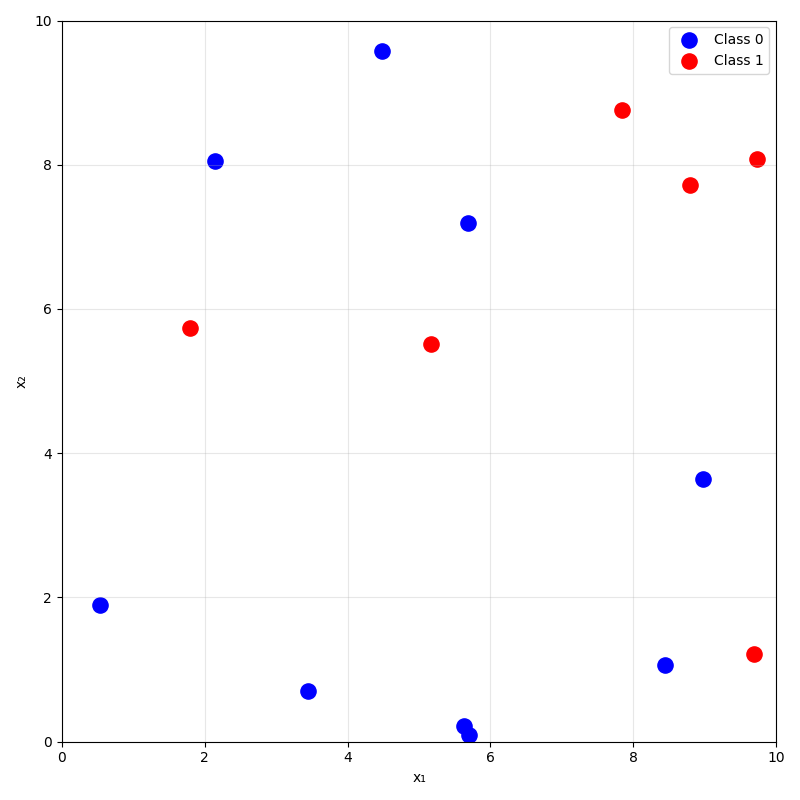
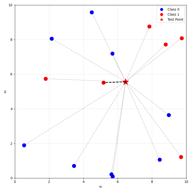
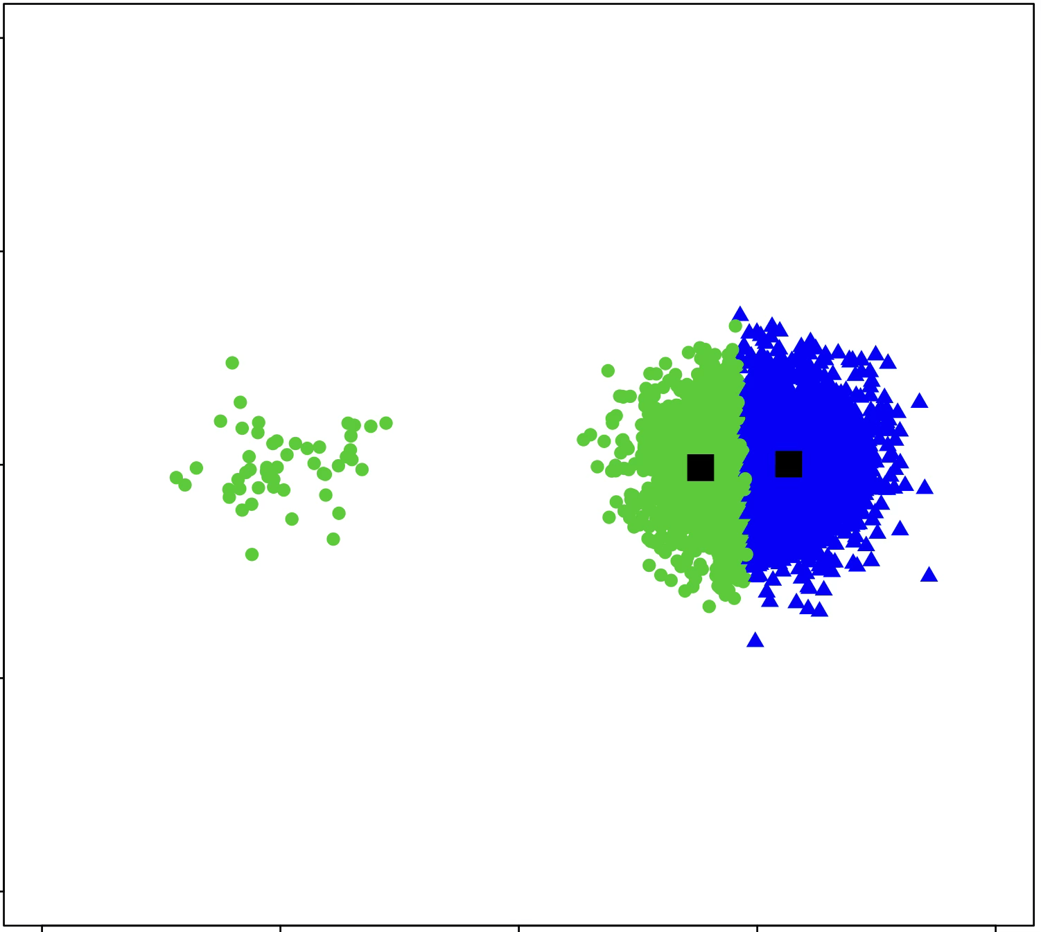
training data
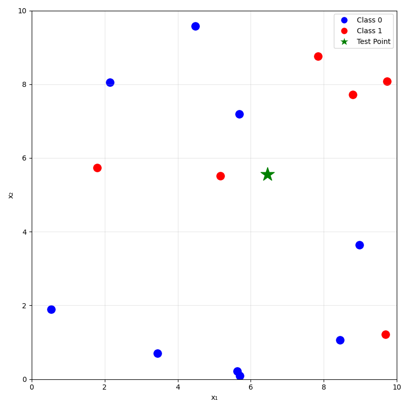
prediction on new data using
\(k=1\) nearest neighbor
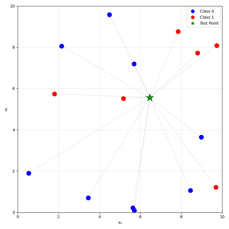
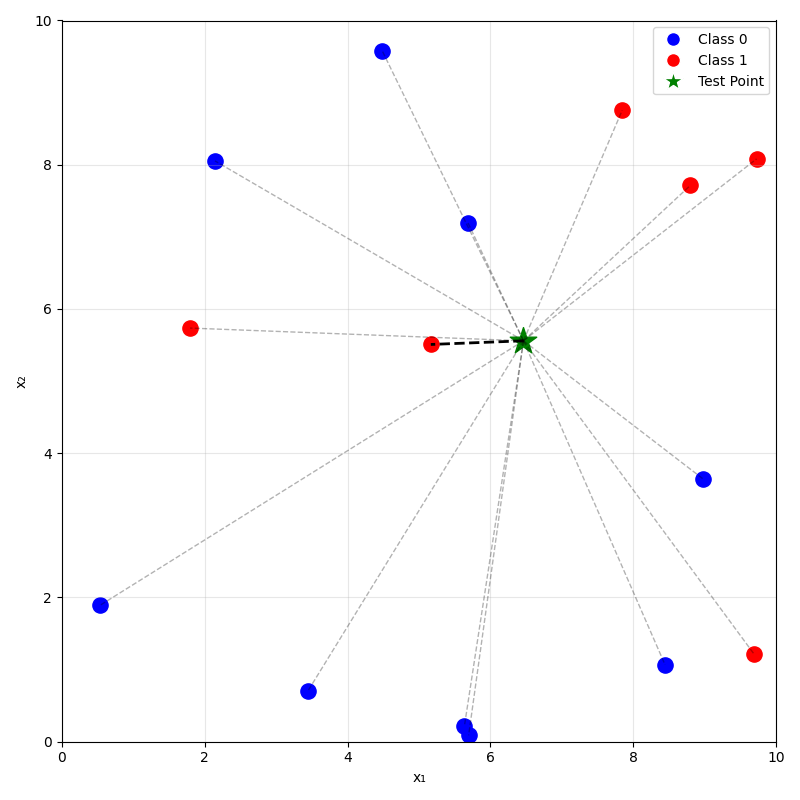


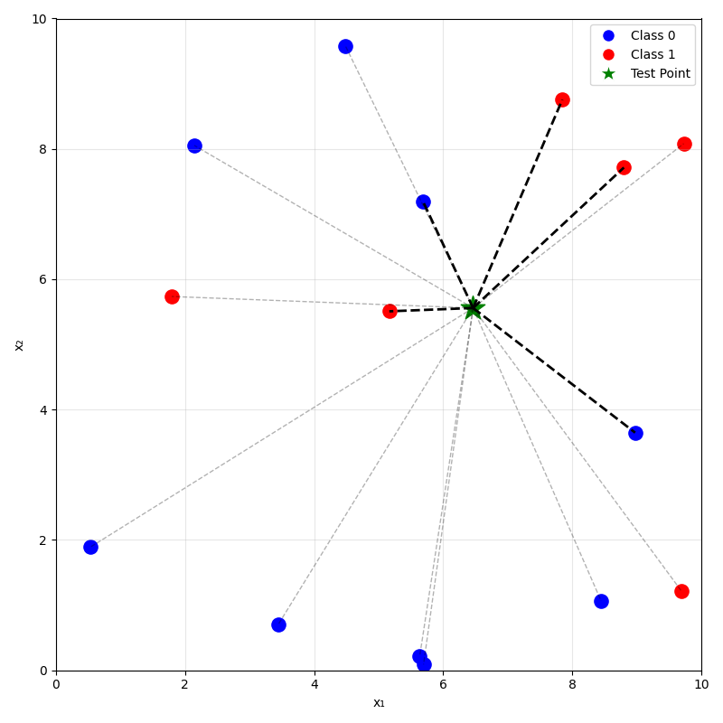
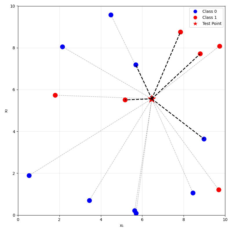
prediction on new data using
\(k=5\) nearest neighbor
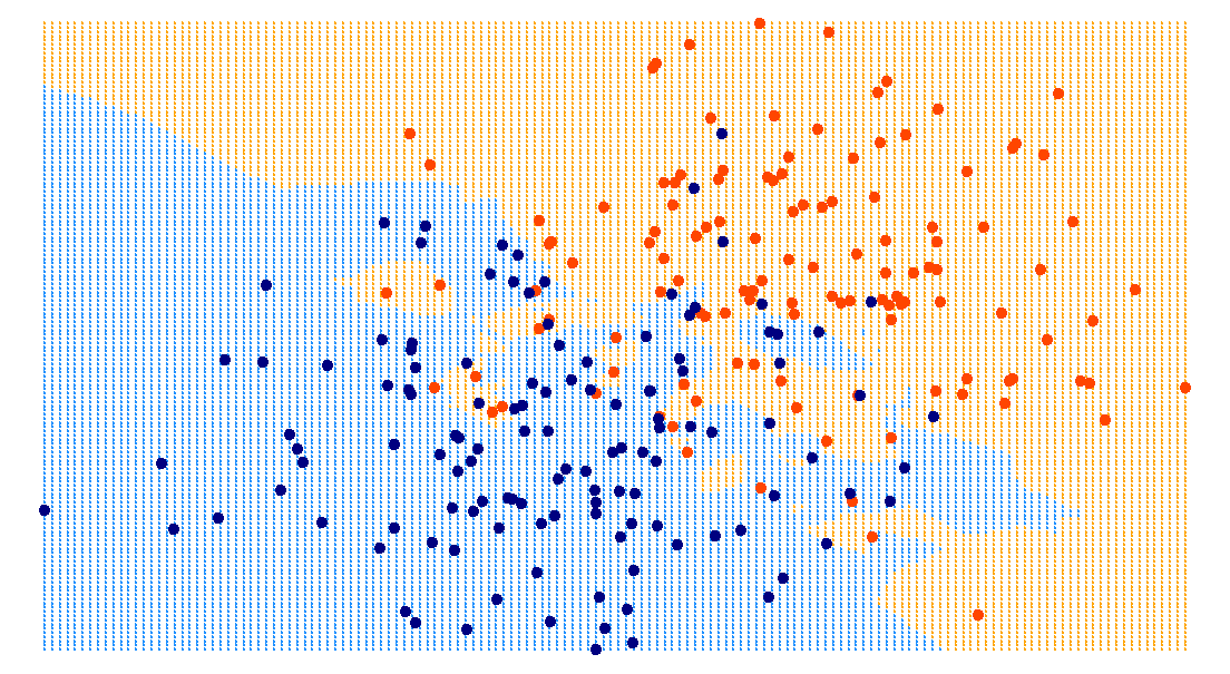

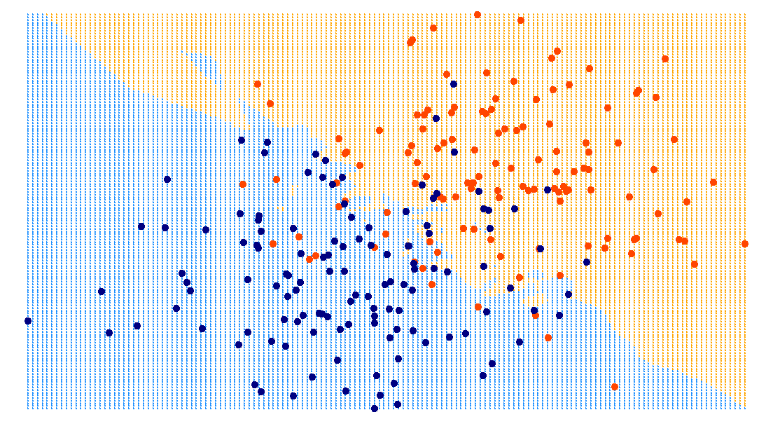
training data
\(k=3\)
\(k=5\)
\(k=10\)
\(x_1\)
\(x_2\)
\(x_1\)
\(x_2\)
\(x_1\)
\(x_2\)
\(x_1\)
\(x_2\)
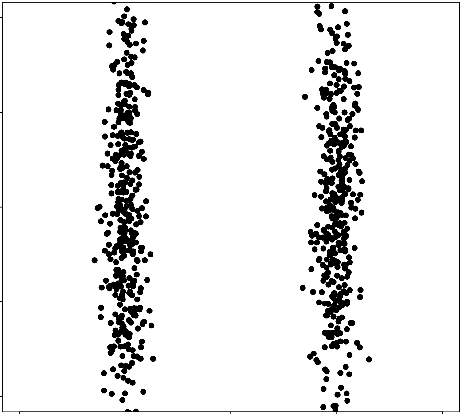
Be cautious when...
- very large \(n\) or \(d\); curse of dimensionality.
- many irrelevant or noisy features.
- features on different scales:
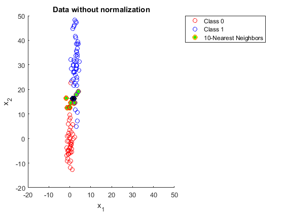
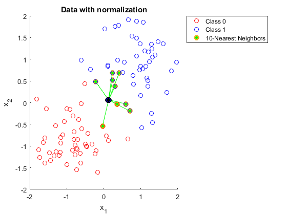
unscaled
scaled
Lewis, Perez, Piktus, et al. Retrieval-Augmented Generation for Knowledge-Intensive NLP Tasks. NeurIPS 2020.
Equip modern language models with a knowledge base
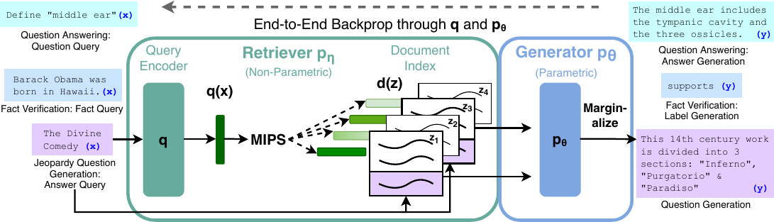
- Build a datastore (key and values) by running one. LM over the entire training corpus.
- At decode time, do k-NN of one query against the datastore keys. The k retrieved values give a kNN distribution over next tokens.
- Interpolate the kNN results with the regular next-token results.
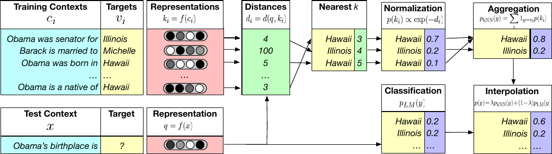
Khandelwal, Levy, Jurafsky, Zettlemoyer, Lewis. Generalization through Memorization: Nearest Neighbor Language Models. ICLR 2020.
Memorization, attached to the model from outside.
Training: none. Just memorize the training set.
Predicting: for a new \(x_{\text{new}}\), take the majority (class) or mean (regression) label of its \(k\) nearest neighbors.
Parameters learned: the entire training set (its features and labels).
Hyperparameters:
- \(k\): number of neighbors considered.
- distance metric (typically Euclidean or Manhattan).
- tie-breaking scheme (typically at random).
Outline
- Non-parametric models overview
-
Similarity-based methods
- \(k\)-nearest neighbor
- \(k\)-means clustering
- Tree-based methods
- Decision Tree
- Bagging and ensembles
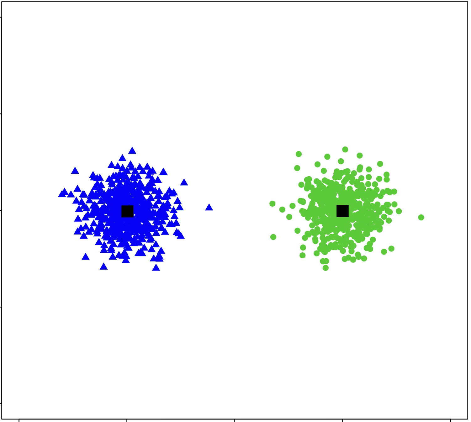
No labeled categories, we can still group by similarities.

(I'm actually not sure of the answers..)
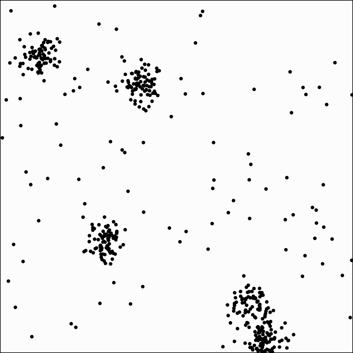
\(k\)-means clustering
structure discovery without labels
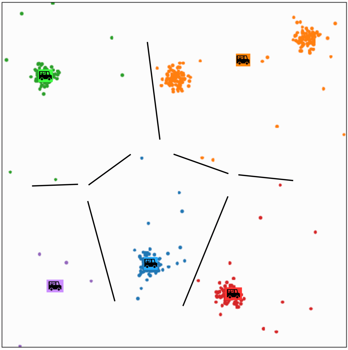
Food-truck placement
- \(x_1\): longitude, \(x_2\): latitude
- \(n\) people, person \(i\) at location \(x^{(i)}\)
- \(k\) food trucks (say \(k=5\))
- truck \(j\) at location \(\mu^{(j)}\)
Per-person loss
Cost for person \(i\) to walk to truck \(j\):
\(\big\|x^{(i)} - \mu^{(j)}\big\|^2\)
Let \(y^{(i)}\) be the truck person \(i\) walks to.
\(\mathbf{1}\{y^{(i)} = j\}\) is 1 if assigned, 0 otherwise.
Person \(i\)'s loss:
\(\sum_{j=1}^{k} \mathbf{1}\{y^{(i)} = j\}\, \big\|x^{(i)} - \mu^{(j)}\big\|^2\)
\( \sum_{j=1}^k \mathbf{1}\left\{y^{(i)}=j\right\}\left\|x^{(i)}-\mu^{(j)}\right\|^2\)
\(k\)-means objective
cluster membership
centroid location
sum over cluster
sum over data points
what we learn
\(\sum_{i=1}^n\)
K-MEANS\((k, \tau, \left\{x^{(i)}\right\}_{i=1}^n)\)
1 \(\mu, y=\) random initialization
2 for \(t=1\) to \(\tau\)
4 for \(i=1\) to \(n\)
\(5 \quad \quad\quad\quad \quad y^{(i)}=\arg \min _j\left\|x^{(i)}-\mu^{(j)}\right\|^2\)
6 for \(j=1\) to \(k\)
\(7 \quad \quad\quad\quad \quad \mu^{(j)}=\frac{1}{N_j} \sum_{i=1}^n \mathbf{1}\left(y^{(i)}=\mathfrak{j}\right) x^{(i)}\)
8 if \(y==y_{\text {old }}\)
9\(\quad \quad \quad\quad \quad\)break
10 return \(\mu, y\)
3 \(y_{\text {old }} = y\)
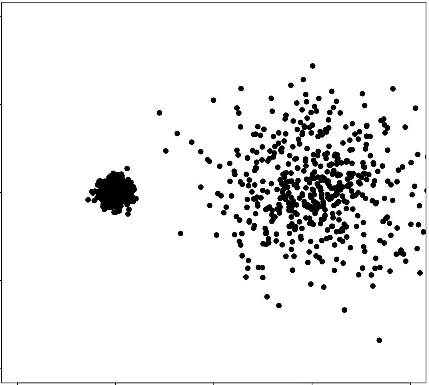
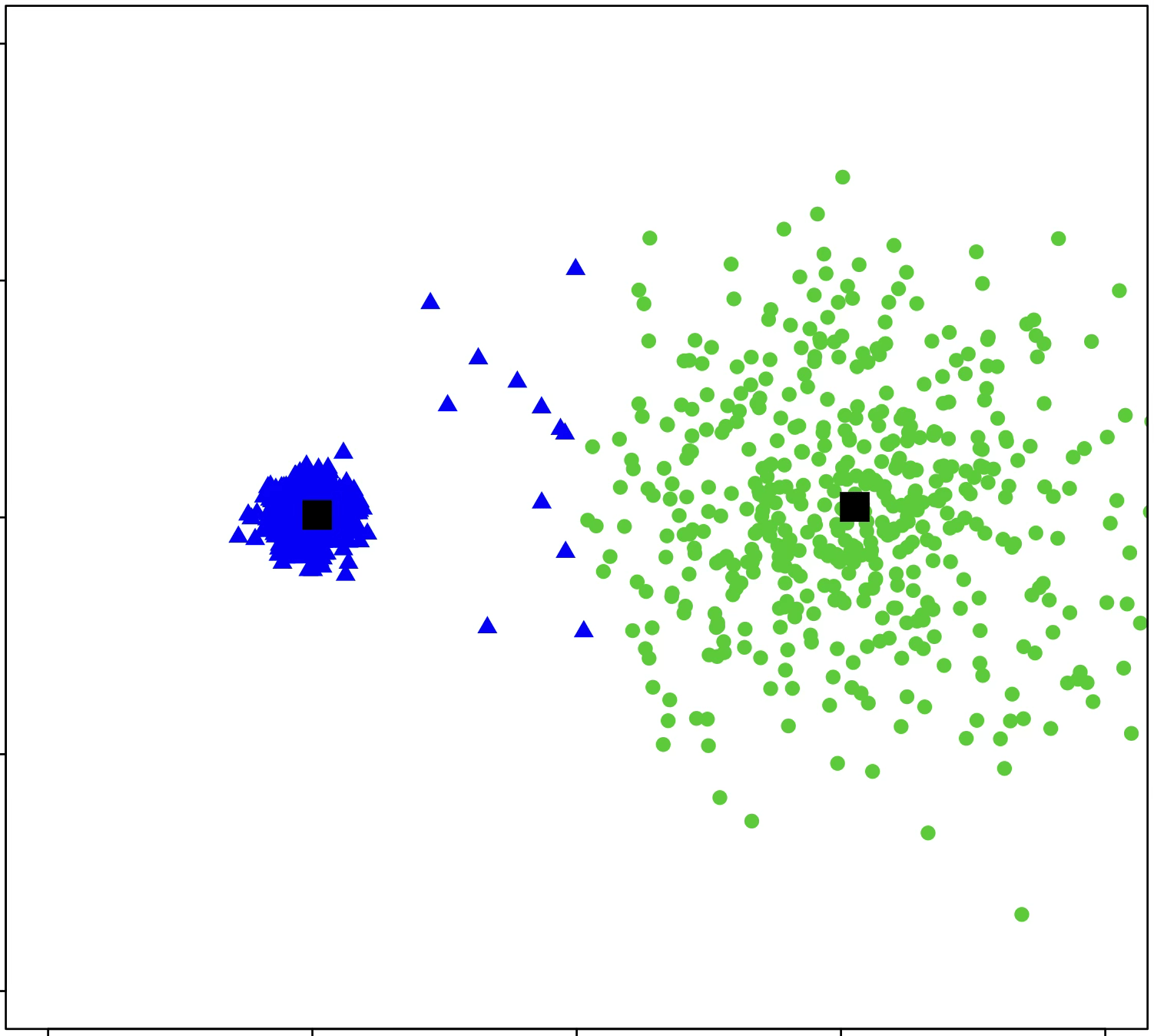
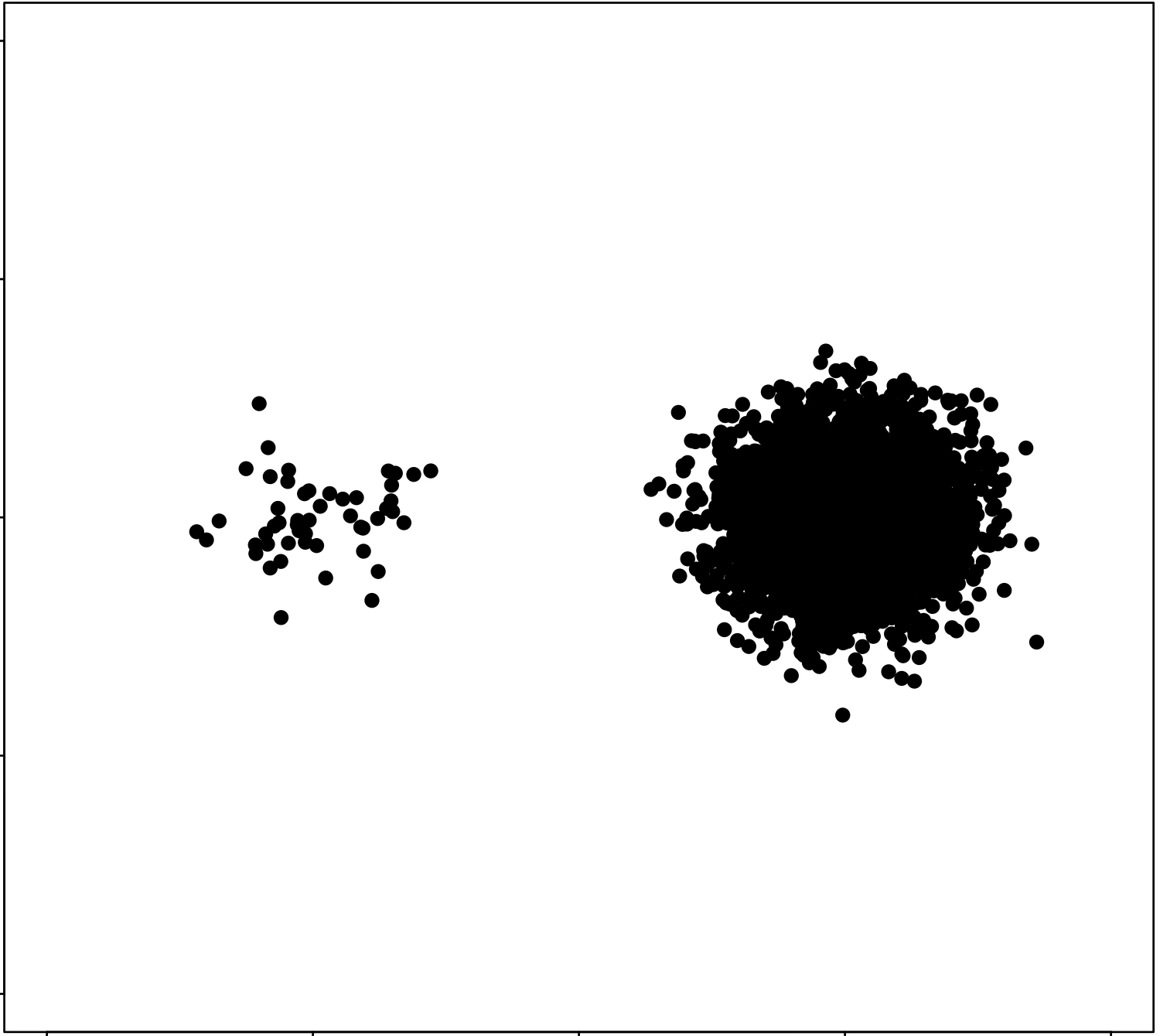
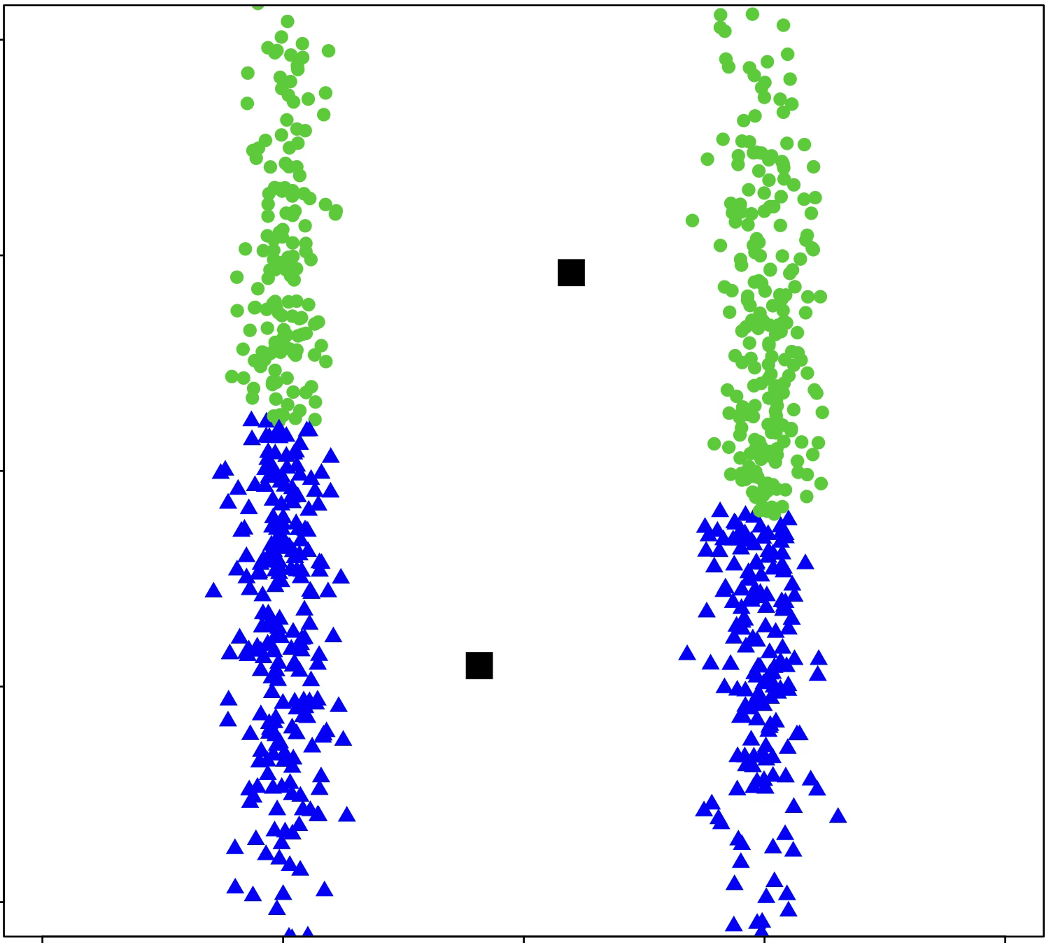
\(k\)-means is sensitive to initialization and to \(k\)
same data, three different initializations:
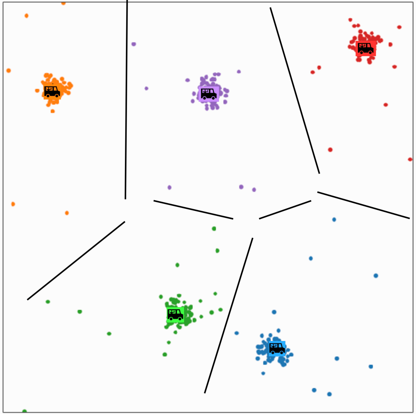
same data, two different choices of \(k\):
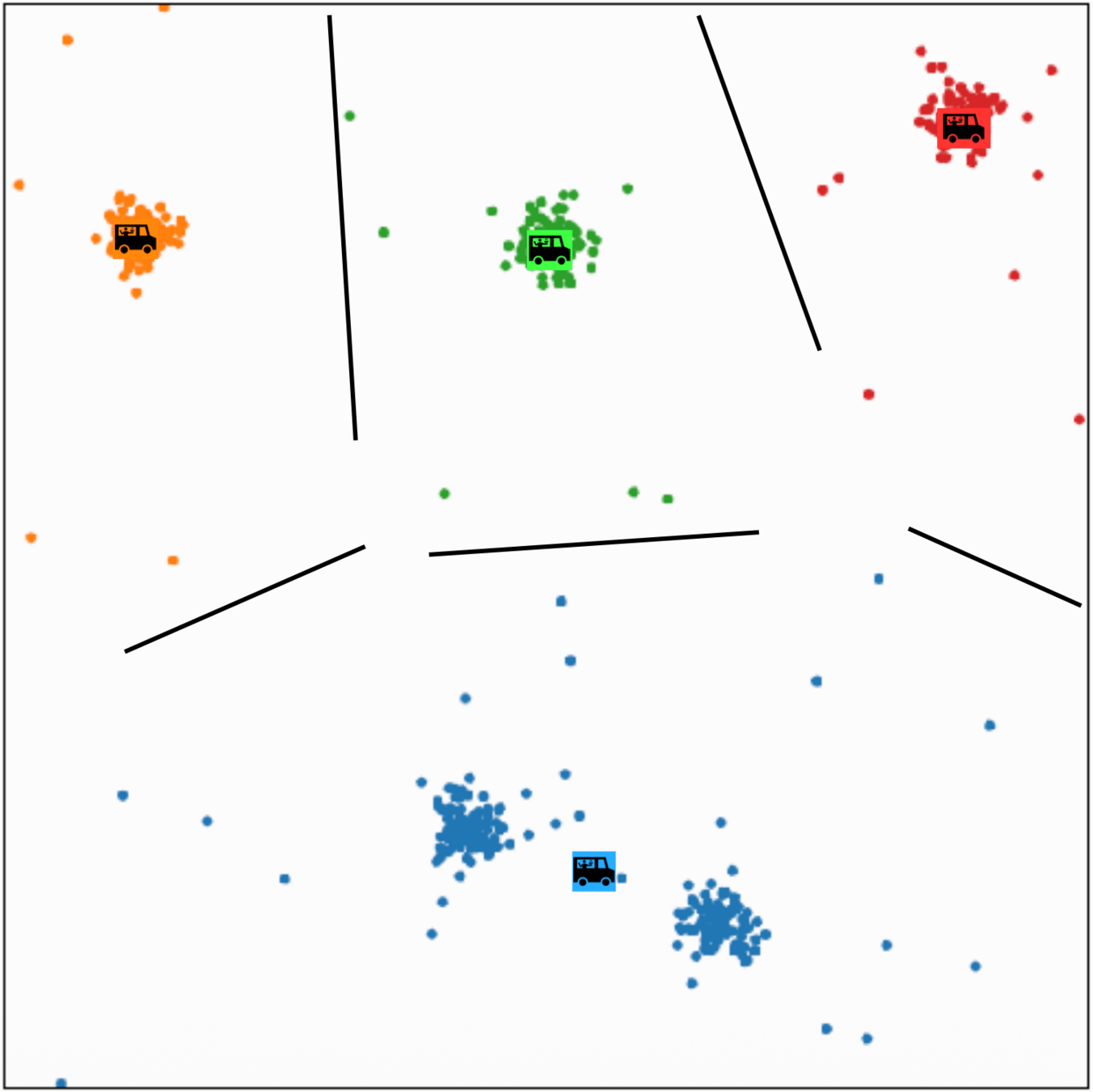
(\(k\)-means works well for well-separated circular clusters of the same size)
- Each cell becomes a high-dim RNA-expression vector.
- Clustering those vectors uncovers cell types, including ones we didn't know existed.
- Standard tools builds this in. Routine in tissue atlases (Human Cell Atlas, Tabula Muris).
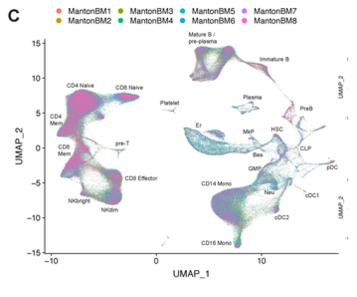
Stuart, Butler, Hoffman, et al. Comprehensive Integration of Single-Cell Data. Cell, 2019 (Seurat v3).
An unsupervised microscope, run in feature space.
\(k\)-means interpreted as a discrete autoencoder
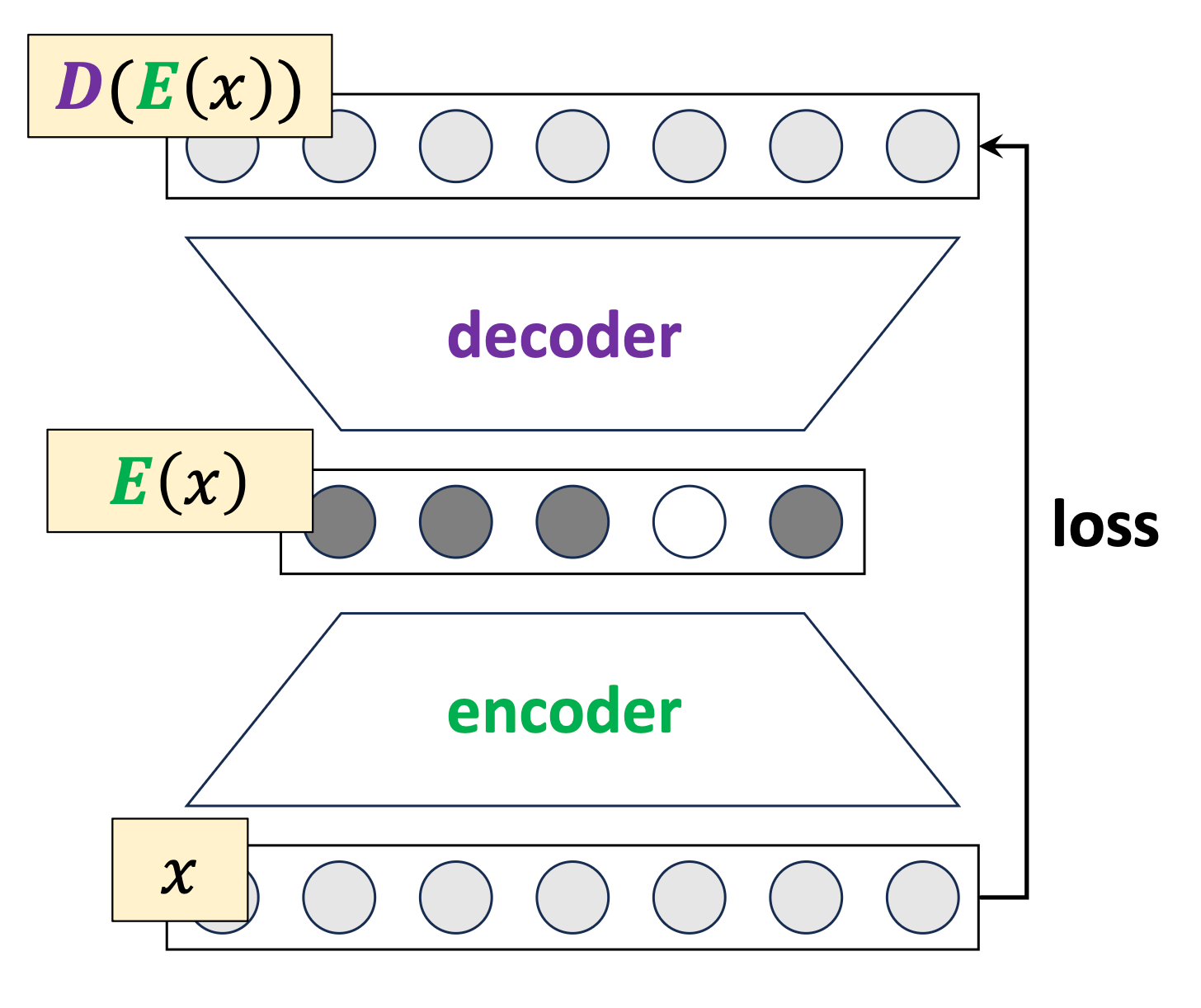
map 𝑥 to a one-hot
map the one-hot to a center
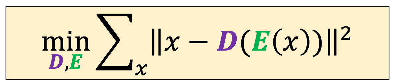
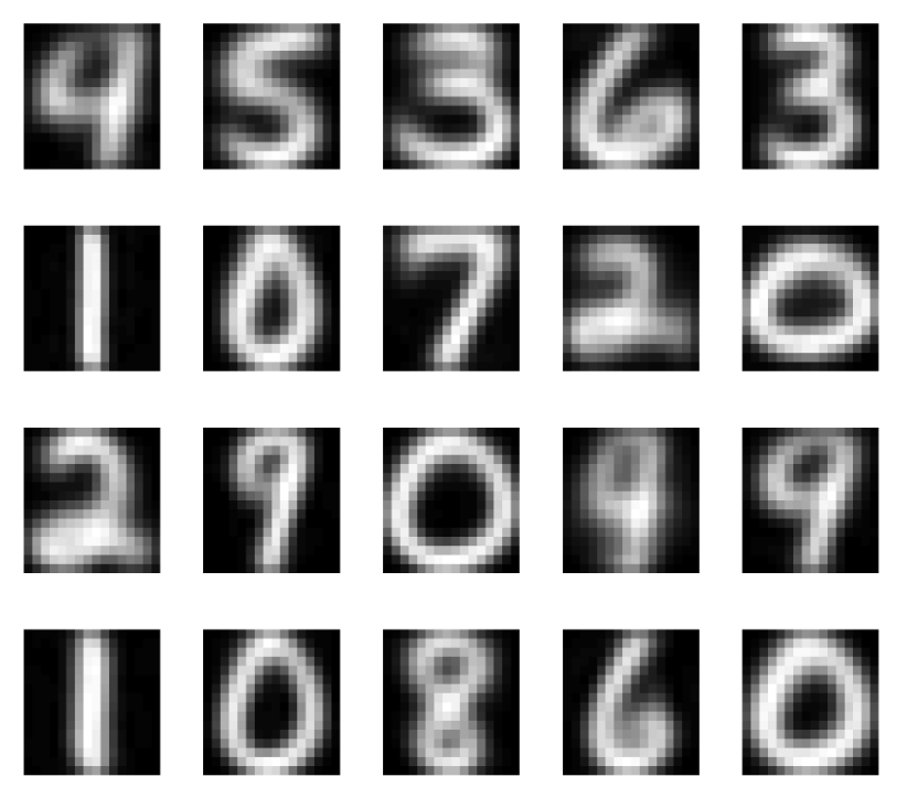
cluster center:
- not actual data points in MNIST
- learned representation and prototypes
Codebooks inside generative models
- VQ-VAE quantizes each encoder output to its nearest codebook vector. The codebook is exactly a set of kk centroids learned from the data.
- Same idea elsewhere: VQGAN, DALL-E for images; SoundStream, EnCodec (used in MusicGen) for audio.
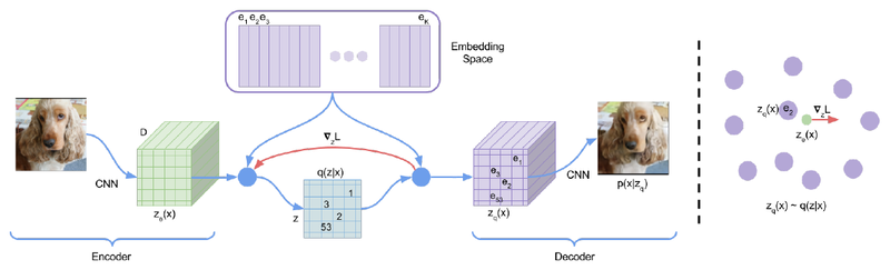
van den Oord, Vinyals, Kavukcuoglu. Neural Discrete Representation Learning. NeurIPS 2017.
- Train a sparse autoencoder on a transformer's hidden states; sparsity makes features behave as discrete prototypes.
- Concepts emerge: Arabic-script tokens, base64 strings, code patterns, locations, emotions.
- Anthropic scaled this to Claude 3. Shares the same high-level instinct as k-means (store small set of meaningful prototypes).
Bricken, Templeton, Batson, et al. Towards Monosemanticity. Anthropic, 2023.
Group similar things, even when "similar" is a model's internal state.
Outline
- Non-parametric models overview
- Similarity-based methods
- \(k\)-nearest neighbor
- \(k\)-means clustering
-
Tree-based methods
- Decision Tree
- Bagging and ensembles
Reading a classification decision tree
features:
\(x_1\) : date
\(x_2\) : age
\(x_3\) : height
\(x_4\) : weight
\(x_5\) : sinus tachycardia?
\(x_6\) : min systolic bp, 24h
\(x_7\) : latest diastolic bp
labels \(y\) :
1: high risk
0: low risk
Each internal node carries a split dimension and split value (\(x_j \geq \theta\)).
Each leaf corresponds to an axis-aligned region; the tree predicts the leaf's value there.
Tree root node, internal node, leaf, and depth
How to Grow a Regression Tree
-
Grow — start with all data at the root.
Try candidate splits along each feature. -
Split — pick the split that best reduces prediction error
(lowest weighted variance of target values). -
Recurse — treat each child region as a whole new dataset and run the algorithm again.
-
Stop — if a region is small or already consistent
(data within ≤ leaf size, or variance below a threshold), make it a leaf.
set of indices
hyper-parameter: largest leaf size
maximum number of training datapoints allowed in a leaf
\(\operatorname{BuildTree}(I, k, \mathcal{D})\)
10. Set \(\hat{y}=\) average \(_{i \in I} y^{(i)}\)
1. if \(|I| > k\)
2. for each split dim \(j\) and split value \(s\)
3. Set \(I_{j, s}^{+}=\left\{i \in I \mid x_j^{(i)} \geq s\right\}\)
4. Set \(I_{j, s}^{-}=\left\{i \in I \mid x_j^{(i)}<s\right\}\)
5. Set \(\hat{y}_{j, s}^{+}=\) average \(_{i \in I_{j, s}^{+}} y^{(i)}\)
6. Set \(\hat{y}_{j, s}^{-}=\) average \(_{i \in I_{j, s}^{-}} y^{(i)}\)
7. Set \(E_{j, s}=\sum_{i \in I_{j, s}^{+}}\left(y^{(i)}-\hat{y}_{j, s}^{+}\right)^2+\sum_{i \in I_{j, s}^{-}}\left(y^{(i)}-\hat{y}_{j, s}^{-}\right)^2\)
8. Set \(\left(j^*, s^*\right)=\arg \min _{j, s} E_{j, s}\)
9. else
11. return \(\operatorname{Leaf}\)(leave_value=\(\hat{y})\)
12. return \(\operatorname{Node}\left(j^*, s^*, \operatorname{BuildTree}\left(I_{j^*, s^*}^{-}, k, \mathcal{D}\right), \operatorname{BuildTree}\left(I_{j^*, s^*}^{+}, k, \mathcal{D}\right)\right)\)
- Choose \(k=2\)
- \(\operatorname{BuildTree}(\{1,2,3\};2)\)
- Line 1 true
\(\operatorname{BuildTree}(I, k, \mathcal{D})\)
10. Set \(\hat{y}=\) average \(_{i \in I} y^{(i)}\)
1. if \(|I| > k\)
2. for each split dim \(j\) and split value \(s\)
3. Set \(I_{j, s}^{+}=\left\{i \in I \mid x_j^{(i)} \geq s\right\}\)
4. Set \(I_{j, s}^{-}=\left\{i \in I \mid x_j^{(i)}<s\right\}\)
5. Set \(\hat{y}_{j, s}^{+}=\) average \(_{i \in I_{j, s}^{+}} y^{(i)}\)
6. Set \(\hat{y}_{j, s}^{-}=\) average \(_{i \in I_{j, s}^{-}} y^{(i)}\)
7. Set \(E_{j, s}=\sum_{i \in I_{j, s}^{+}}\left(y^{(i)}-\hat{y}_{j, s}^{+}\right)^2+\sum_{i \in I_{j, s}^{-}}\left(y^{(i)}-\hat{y}_{j, s}^{-}\right)^2\)
8. Set \(\left(j^*, s^*\right)=\arg \min _{j, s} E_{j, s}\)
9. else
11. return \(\operatorname{Leaf}\)(leave_value=\(\hat{y})\)
12. return \(\operatorname{Node}\left(j^*, s^*, \operatorname{BuildTree}\left(I_{j^*, s^*}^{-}, k\right), \operatorname{BuildTree}\left(I_{j^*, s^*}^{+}, k\right)\right)\)
\(\operatorname{BuildTree}(I, k, \mathcal{D})\)
1. if \(|I| > k\)
2. for each split dim \(j\) and split value \(s\)
3. Set \(I_{j, s}^{+}=\left\{i \in I \mid x_j^{(i)} \geq s\right\}\)
4. Set \(I_{j, s}^{-}=\left\{i \in I \mid x_j^{(i)}<s\right\}\)
5. Set \(\hat{y}_{j, s}^{+}=\) average \(_{i \in I_{j, s}^{+}} y^{(i)}\)
6. Set \(\hat{y}_{j, s}^{-}=\) average \(_{i \in I_{j, s}^{-}} y^{(i)}\)
7. Set \(E_{j, s}=\sum_{i \in I_{j, s}^{+}}\left(y^{(i)}-\hat{y}_{j, s}^{+}\right)^2+\sum_{i \in I_{j, s}^{-}}\left(y^{(i)}-\hat{y}_{j, s}^{-}\right)^2\)
8. Set \(\left(j^*, s^*\right)=\arg \min _{j, s} E_{j, s}\)
9. else
10. Set \(\hat{y}=\) average \(_{i \in I} y^{(i)}\)
11. return \(\operatorname{Leaf}\)(leave_value=\(\hat{y})\)
12. return \(\operatorname{Node}\left(j^*, s^*, \operatorname{BuildTree}\left(I_{j^*, s^*}^{-}, k\right), \operatorname{BuildTree}\left(I_{j^*, s^*}^{+}, k\right)\right)\)
- For this fixed \((j, s)\)
- \(I_{j, s}^{+} = \{2,3\}\)
- \(I_{j, s}^{-} = \{1\}\)
- \(\hat{y}_{j, s}^{+} = 5\)
- \(\hat{y}_{j, s}^{-} = 0\)
- \(E_{j, s} =0\)
\(\operatorname{BuildTree}(I, k, \mathcal{D})\)
1. if \(|I| > k\)
2. for each split dim \(j\) and split value \(s\)
3. Set \(I_{j, s}^{+}=\left\{i \in I \mid x_j^{(i)} \geq s\right\}\)
4. Set \(I_{j, s}^{-}=\left\{i \in I \mid x_j^{(i)}<s\right\}\)
5. Set \(\hat{y}_{j, s}^{+}=\) average \(_{i \in I_{j, s}^{+}} y^{(i)}\)
6. Set \(\hat{y}_{j, s}^{-}=\) average \(_{i \in I_{j, s}^{-}} y^{(i)}\)
7. Set \(E_{j, s}=\sum_{i \in I_{j, s}^{+}}\left(y^{(i)}-\hat{y}_{j, s}^{+}\right)^2+\sum_{i \in I_{j, s}^{-}}\left(y^{(i)}-\hat{y}_{j, s}^{-}\right)^2\)
8. Set \(\left(j^*, s^*\right)=\arg \min _{j, s} E_{j, s}\)
9. else
10. Set \(\hat{y}=\) average \(_{i \in I} y^{(i)}\)
11. return \(\operatorname{Leaf}\)(leave_value=\(\hat{y})\)
12. return \(\operatorname{Node}\left(j^*, s^*, \operatorname{BuildTree}\left(I_{j^*, s^*}^{-}, k\right), \operatorname{BuildTree}\left(I_{j^*, s^*}^{+}, k\right)\right)\)
Line 2: suffices to consider a finite number of \((j, s)\)
(those that split in-between data points)
\(\operatorname{BuildTree}(I, k, \mathcal{D})\)
1. if \(|I| > k\)
2. for each split dim \(j\) and split value \(s\)
3. Set \(I_{j, s}^{+}=\left\{i \in I \mid x_j^{(i)} \geq s\right\}\)
4. Set \(I_{j, s}^{-}=\left\{i \in I \mid x_j^{(i)}<s\right\}\)
5. Set \(\hat{y}_{j, s}^{+}=\) average \(_{i \in I_{j, s}^{+}} y^{(i)}\)
6. Set \(\hat{y}_{j, s}^{-}=\) average \(_{i \in I_{j, s}^{-}} y^{(i)}\)
7. Set \(E_{j, s}=\sum_{i \in I_{j, s}^{+}}\left(y^{(i)}-\hat{y}_{j, s}^{+}\right)^2+\sum_{i \in I_{j, s}^{-}}\left(y^{(i)}-\hat{y}_{j, s}^{-}\right)^2\)
8. Set \(\left(j^*, s^*\right)=\arg \min _{j, s} E_{j, s}\)
9. else
10. Set \(\hat{y}=\) average \(_{i \in I} y^{(i)}\)
11. return \(\operatorname{Leaf}\)(leave_value=\(\hat{y})\)
12. return \(\operatorname{Node}\left(j^*, s^*, \operatorname{BuildTree}\left(I_{j^*, s^*}^{-}, k\right), \operatorname{BuildTree}\left(I_{j^*, s^*}^{+}, k\right)\right)\)
Line 8: picks the "best" among these finite choices of \((j, s)\) combos (random tie-breaking).
\(\operatorname{BuildTree}(I, k, \mathcal{D})\)
1. if \(|I| > k\)
2. for each split dim \(j\) and split value \(s\)
3. Set \(I_{j, s}^{+}=\left\{i \in I \mid x_j^{(i)} \geq s\right\}\)
4. Set \(I_{j, s}^{-}=\left\{i \in I \mid x_j^{(i)}<s\right\}\)
5. Set \(\hat{y}_{j, s}^{+}=\) average \(_{i \in I_{j, s}^{+}} y^{(i)}\)
6. Set \(\hat{y}_{j, s}^{-}=\) average \(_{i \in I_{j, s}^{-}} y^{(i)}\)
7. Set \(E_{j, s}=\sum_{i \in I_{j, s}^{+}}\left(y^{(i)}-\hat{y}_{j, s}^{+}\right)^2+\sum_{i \in I_{j, s}^{-}}\left(y^{(i)}-\hat{y}_{j, s}^{-}\right)^2\)
8. Set \(\left(j^*, s^*\right)=\arg \min _{j, s} E_{j, s}\)
9. else
10. Set \(\hat{y}=\) average \(_{i \in I} y^{(i)}\)
11. return \(\operatorname{Leaf}\)(leave_value=\(\hat{y})\)
12. return \(\operatorname{Node}\left(j^*, s^*, \operatorname{BuildTree}\left(I_{j^*, s^*}^{-}, k\right), \operatorname{BuildTree}\left(I_{j^*, s^*}^{+}, k\right)\right)\)
Suppose line 8 sets this \((j^*,s^*)\),
say \((j^*,s^*) = (1, 1.7)\)
\(\operatorname{BuildTree}(I, k, \mathcal{D})\)
1. if \(|I| > k\)
2. for each split dim \(j\) and split value \(s\)
3. Set \(I_{j, s}^{+}=\left\{i \in I \mid x_j^{(i)} \geq s\right\}\)
4. Set \(I_{j, s}^{-}=\left\{i \in I \mid x_j^{(i)}<s\right\}\)
5. Set \(\hat{y}_{j, s}^{+}=\) average \(_{i \in I_{j, s}^{+}} y^{(i)}\)
6. Set \(\hat{y}_{j, s}^{-}=\) average \(_{i \in I_{j, s}^{-}} y^{(i)}\)
7. Set \(E_{j, s}=\sum_{i \in I_{j, s}^{+}}\left(y^{(i)}-\hat{y}_{j, s}^{+}\right)^2+\sum_{i \in I_{j, s}^{-}}\left(y^{(i)}-\hat{y}_{j, s}^{-}\right)^2\)
8. Set \(\left(j^*, s^*\right)=\arg \min _{j, s} E_{j, s}\)
9. else
10. Set \(\hat{y}=\) average \(_{i \in I} y^{(i)}\)
11. return \(\operatorname{Leaf}\)(leave_value=\(\hat{y})\)
12. return \(\operatorname{Node}\left(j^*, s^*, \operatorname{BuildTree}\left(I_{j^*, s^*}^{-}, k\right), \operatorname{BuildTree}\left(I_{j^*, s^*}^{+}, k\right)\right)\)
Line 12, do recursion
\(x_1 \geq 1.7\)
\(\operatorname{BuildTree}(I, k, \mathcal{D})\)
1. if \(|I| > k\)
2. for each split dim \(j\) and split value \(s\)
3. Set \(I_{j, s}^{+}=\left\{i \in I \mid x_j^{(i)} \geq s\right\}\)
4. Set \(I_{j, s}^{-}=\left\{i \in I \mid x_j^{(i)}<s\right\}\)
5. Set \(\hat{y}_{j, s}^{+}=\) average \(_{i \in I_{j, s}^{+}} y^{(i)}\)
6. Set \(\hat{y}_{j, s}^{-}=\) average \(_{i \in I_{j, s}^{-}} y^{(i)}\)
7. Set \(E_{j, s}=\sum_{i \in I_{j, s}^{+}}\left(y^{(i)}-\hat{y}_{j, s}^{+}\right)^2+\sum_{i \in I_{j, s}^{-}}\left(y^{(i)}-\hat{y}_{j, s}^{-}\right)^2\)
8. Set \(\left(j^*, s^*\right)=\arg \min _{j, s} E_{j, s}\)
9. else
10. Set \(\hat{y}=\) average \(_{i \in I} y^{(i)}\)
11. return \(\operatorname{Leaf}\)(leave_value=\(\hat{y})\)
12. return \(\operatorname{Node}\left(j^*, s^*, \operatorname{BuildTree}\left(I_{j^*, s^*}^{-}, k\right), \operatorname{BuildTree}\left(I_{j^*, s^*}^{+}, k\right)\right)\)
\(x_1 \geq 1.7\)
0
5
How to Grow a Classification Tree
-
Grow — start with all data at the root.
Try candidate splits along each feature. -
Split — pick the split that best separates the classes
(lowest weighted entropy or most "homogeneous"). -
Recurse — treat each child region as a whole new dataset and run the algorithm again.
-
Stop — if a region is small or already pure
(data within ≤ leaf size, or most data share the same label), make it a leaf.
entropy \(H:=-\sum_{\text {class }_c} \hat{P}_c (\log _2 \hat{P}_c)\)
(about 1.1)
for example: \(c\) iterates over 3 classes
\(\hat{P}_c:\)
\(H= -[\frac{4}{6} \log _2\left(\frac{4}{6}\right)+\frac{1}{6} \log _2\left(\frac{1}{6}\right)+\frac{1}{6} \log _2\left(\frac{1}{6}\right)]\)
(about 1.252)
\(\hat{P}_c:\)
\(H= -[\frac{3}{6} \log _2\left(\frac{3}{6}\right)+\frac{3}{6} \log _2\left(\frac{3}{6}\right)+ 0]\)
\(\hat{P}_c:\)
\(H= -[\frac{6}{6} \log _2\left(\frac{6}{6}\right)+ 0+ 0]\)
(= 0)
empirical probability
\(\operatorname{BuildTree}(I, k, \mathcal{D})\)
10. Set \(\hat{y}=\) majority \(_{i \in I} y^{(i)}\)
1. if \(|I| > k\)
2. for each split dim \(j\) and split value \(s\)
3. Set \(I_{j, s}^{+}=\left\{i \in I \mid x_j^{(i)} \geq s\right\}\)
4. Set \(I_{j, s}^{-}=\left\{i \in I \mid x_j^{(i)}<s\right\}\)
5. Set \(\hat{y}_{j, s}^{+}=\) majority \(_{i \in I_{j, s}^{+}} y^{(i)}\)
6. Set \(\hat{y}_{j, s}^{-}=\) majority \(_{i \in I_{j, s}^{-}} y^{(i)}\)
7. Set \(E_{j, s} = \frac{\left|I_{j, s}^{-}\right|}{|I|} \cdot H\left(I_{j, s}^{-}\right)+\frac{\left|I_{j, s}^{+}\right|}{|I|} \cdot H\left(I_{j, s}^{+}\right)\)
8. Set \(\left(j^*, s^*\right)=\arg \min _{j, s} E_{j, s}\)
9. else
11. return \(\operatorname{Leaf}\)(leave_value=\(\hat{y})\)
12. return \(\operatorname{Node}\left(j^*, s^*, \operatorname{BuildTree}\left(I_{j^*, s^*}^{-}, k\right), \operatorname{BuildTree}\left(I_{j^*, s^*}^{+}, k\right)\right)\)
weighted average entropy (WAE)
as performance metric
majority vote
as regional prediction
For classification
\(\operatorname{BuildTree}(I, k, \mathcal{D})\)
10. Set \(\hat{y}=\) majority \(_{i \in I} y^{(i)}\)
1. if \(|I| > k\)
2. for each split dim \(j\) and split value \(s\)
3. Set \(I_{j, s}^{+}=\left\{i \in I \mid x_j^{(i)} \geq s\right\}\)
4. Set \(I_{j, s}^{-}=\left\{i \in I \mid x_j^{(i)}<s\right\}\)
5. Set \(\hat{y}_{j, s}^{+}=\) majority \(_{i \in I_{j, s}^{+}} y^{(i)}\)
6. Set \(\hat{y}_{j, s}^{-}=\) majority \(_{i \in I_{j, s}^{-}} y^{(i)}\)
7. Set \(E_{j, s} = \frac{\left|I_{j, s}^{-}\right|}{|I|} \cdot H\left(I_{j, s}^{-}\right)+\frac{\left|I_{j, s}^{+}\right|}{|I|} \cdot H\left(I_{j, s}^{+}\right)\)
8. Set \(\left(j^*, s^*\right)=\arg \min _{j, s} E_{j, s}\)
9. else
11. return \(\operatorname{Leaf}\)(leave_value=\(\hat{y})\)
12. return \(\operatorname{Node}\left(j^*, s^*, \operatorname{BuildTree}\left(I_{j^*, s^*}^{-}, k\right), \operatorname{BuildTree}\left(I_{j^*, s^*}^{+}, k\right)\right)\)
\( \frac{4}{6} \cdot H\left(I_{j, s}^{-}\right)+\frac{2}{6} \cdot H\left(I_{j, s}^{+}\right)\)
fraction of points to the left of the split
fraction of points to the right of the split
\(E_{j,s}= \)
\(\operatorname{BuildTree}(I, k, \mathcal{D})\)
10. Set \(\hat{y}=\) majority \(_{i \in I} y^{(i)}\)
1. if \(|I| > k\)
2. for each split dim \(j\) and split value \(s\)
3. Set \(I_{j, s}^{+}=\left\{i \in I \mid x_j^{(i)} \geq s\right\}\)
4. Set \(I_{j, s}^{-}=\left\{i \in I \mid x_j^{(i)}<s\right\}\)
5. Set \(\hat{y}_{j, s}^{+}=\) majority \(_{i \in I_{j, s}^{+}} y^{(i)}\)
6. Set \(\hat{y}_{j, s}^{-}=\) majority \(_{i \in I_{j, s}^{-}} y^{(i)}\)
7. Set \(E_{j, s} = \frac{\left|I_{j, s}^{-}\right|}{|I|} \cdot H\left(I_{j, s}^{-}\right)+\frac{\left|I_{j, s}^{+}\right|}{|I|} \cdot H\left(I_{j, s}^{+}\right)\)
8. Set \(\left(j^*, s^*\right)=\arg \min _{j, s} E_{j, s}\)
9. else
11. return \(\operatorname{Leaf}\)(leave_value=\(\hat{y})\)
12. return \(\operatorname{Node}\left(j^*, s^*, \operatorname{BuildTree}\left(I_{j^*, s^*}^{-}, k\right), \operatorname{BuildTree}\left(I_{j^*, s^*}^{+}, k\right)\right)\)
\( -[\frac{3}{4} \log _2\left(\frac{3}{4}\right)+\frac{1}{4} \log _2\left(\frac{1}{4}\right)+0] \approx 0.811\)
\( \frac{4}{6} \cdot H\left(I_{j, s}^{-}\right)+\frac{2}{6} \cdot H\left(I_{j, s}^{+}\right)\)
\(\hat{P}_c:\)
\(\operatorname{BuildTree}(I, k, \mathcal{D})\)
10. Set \(\hat{y}=\) majority \(_{i \in I} y^{(i)}\)
1. if \(|I| > k\)
2. for each split dim \(j\) and split value \(s\)
3. Set \(I_{j, s}^{+}=\left\{i \in I \mid x_j^{(i)} \geq s\right\}\)
4. Set \(I_{j, s}^{-}=\left\{i \in I \mid x_j^{(i)}<s\right\}\)
5. Set \(\hat{y}_{j, s}^{+}=\) majority \(_{i \in I_{j, s}^{+}} y^{(i)}\)
6. Set \(\hat{y}_{j, s}^{-}=\) majority \(_{i \in I_{j, s}^{-}} y^{(i)}\)
7. Set \(E_{j, s} = \frac{\left|I_{j, s}^{-}\right|}{|I|} \cdot H\left(I_{j, s}^{-}\right)+\frac{\left|I_{j, s}^{+}\right|}{|I|} \cdot H\left(I_{j, s}^{+}\right)\)
8. Set \(\left(j^*, s^*\right)=\arg \min _{j, s} E_{j, s}\)
9. else
11. return \(\operatorname{Leaf}\)(leave_value=\(\hat{y})\)
12. return \(\operatorname{Node}\left(j^*, s^*, \operatorname{BuildTree}\left(I_{j^*, s^*}^{-}, k\right), \operatorname{BuildTree}\left(I_{j^*, s^*}^{+}, k\right)\right)\)
\( \frac{4}{6} \cdot H\left(I_{j, s}^{-}\right)+\frac{2}{6} \cdot H\left(I_{j, s}^{+}\right)\)
\(\approx 0.811\)
\( -[\frac{1}{2} \log _2\left(\frac{1}{2}\right)+\frac{1}{2} \log _2\left(\frac{1}{2}\right)+0] = 1\)
\(\hat{P}_c:\)
\(\operatorname{BuildTree}(I, k, \mathcal{D})\)
10. Set \(\hat{y}=\) majority \(_{i \in I} y^{(i)}\)
1. if \(|I| > k\)
2. for each split dim \(j\) and split value \(s\)
3. Set \(I_{j, s}^{+}=\left\{i \in I \mid x_j^{(i)} \geq s\right\}\)
4. Set \(I_{j, s}^{-}=\left\{i \in I \mid x_j^{(i)}<s\right\}\)
5. Set \(\hat{y}_{j, s}^{+}=\) majority \(_{i \in I_{j, s}^{+}} y^{(i)}\)
6. Set \(\hat{y}_{j, s}^{-}=\) majority \(_{i \in I_{j, s}^{-}} y^{(i)}\)
7. Set \(E_{j, s} = \frac{\left|I_{j, s}^{-}\right|}{|I|} \cdot H\left(I_{j, s}^{-}\right)+\frac{\left|I_{j, s}^{+}\right|}{|I|} \cdot H\left(I_{j, s}^{+}\right)\)
8. Set \(\left(j^*, s^*\right)=\arg \min _{j, s} E_{j, s}\)
9. else
11. return \(\operatorname{Leaf}\)(leave_value=\(\hat{y})\)
12. return \(\operatorname{Node}\left(j^*, s^*, \operatorname{BuildTree}\left(I_{j^*, s^*}^{-}, k\right), \operatorname{BuildTree}\left(I_{j^*, s^*}^{+}, k\right)\right)\)
\( \frac{4}{6} \cdot H\left(I_{j, s}^{-}\right)+\frac{2}{6} \cdot H\left(I_{j, s}^{+}\right)\)
\(\approx 0.811\)
\( = 1\)
(for this split choice, line 7 \(E_{j, s}\approx\) 0.874)
\(\approx \frac{4}{6}\cdot0.811+\frac{2}{6}\cdot 1\)
\(= 0.874\)
\(\operatorname{BuildTree}(I, k, \mathcal{D})\)
10. Set \(\hat{y}=\) majority \(_{i \in I} y^{(i)}\)
1. if \(|I| > k\)
2. for each split dim \(j\) and split value \(s\)
3. Set \(I_{j, s}^{+}=\left\{i \in I \mid x_j^{(i)} \geq s\right\}\)
4. Set \(I_{j, s}^{-}=\left\{i \in I \mid x_j^{(i)}<s\right\}\)
5. Set \(\hat{y}_{j, s}^{+}=\) majority \(_{i \in I_{j, s}^{+}} y^{(i)}\)
6. Set \(\hat{y}_{j, s}^{-}=\) majority \(_{i \in I_{j, s}^{-}} y^{(i)}\)
7. Set \(E_{j, s} = \frac{\left|I_{j, s}^{-}\right|}{|I|} \cdot H\left(I_{j, s}^{-}\right)+\frac{\left|I_{j, s}^{+}\right|}{|I|} \cdot H\left(I_{j, s}^{+}\right)\)
8. Set \(\left(j^*, s^*\right)=\arg \min _{j, s} E_{j, s}\)
9. else
11. return \(\operatorname{Leaf}\)(leave_value=\(\hat{y})\)
12. return \(\operatorname{Node}\left(j^*, s^*, \operatorname{BuildTree}\left(I_{j^*, s^*}^{-}, k\right), \operatorname{BuildTree}\left(I_{j^*, s^*}^{+}, k\right)\right)\)
\( \frac{5}{6} \cdot H\left(I_{j, s}^{-}\right)+\frac{1}{6} \cdot H\left(I_{j, s}^{+}\right)\)
\( -[\frac{4}{5} \log _2\left(\frac{4}{5}\right)+\frac{1}{5} \log _2\left(\frac{1}{5}\right)+0] \approx 0.722\)
\( -[1 \log _2\left(1\right)+0+0] = 0\)
(line 7, overall \(E_{j, s}\approx\) 0.602)
\(\operatorname{BuildTree}(I, k, \mathcal{D})\)
10. Set \(\hat{y}=\) majority \(_{i \in I} y^{(i)}\)
1. if \(|I| > k\)
2. for each split dim \(j\) and split value \(s\)
3. Set \(I_{j, s}^{+}=\left\{i \in I \mid x_j^{(i)} \geq s\right\}\)
4. Set \(I_{j, s}^{-}=\left\{i \in I \mid x_j^{(i)}<s\right\}\)
5. Set \(\hat{y}_{j, s}^{+}=\) majority \(_{i \in I_{j, s}^{+}} y^{(i)}\)
6. Set \(\hat{y}_{j, s}^{-}=\) majority \(_{i \in I_{j, s}^{-}} y^{(i)}\)
7. Set \(E_{j, s} = \frac{\left|I_{j, s}^{-}\right|}{|I|} \cdot H\left(I_{j, s}^{-}\right)+\frac{\left|I_{j, s}^{+}\right|}{|I|} \cdot H\left(I_{j, s}^{+}\right)\)
8. Set \(\left(j^*, s^*\right)=\arg \min _{j, s} E_{j, s}\)
9. else
11. return \(\operatorname{Leaf}\)(leave_value=\(\hat{y})\)
12. return \(\operatorname{Node}\left(j^*, s^*, \operatorname{BuildTree}\left(I_{j^*, s^*}^{-}, k\right), \operatorname{BuildTree}\left(I_{j^*, s^*}^{+}, k\right)\right)\)
this split \(E_{j, s}\approx\) 0.602
this split \(E_{j, s}\approx\) 0.874
line 8, set the better \((j, s)\)

Ensemble: Train multiple (diverse) models, combine their predictions


Bagging =
Bootstrap aggregating
Training data \(\mathcal{D}_n\)
\(\left(x^{(1)}, y^{(1)}\right)\)
\(\left(x^{(2)}, y^{(2)}\right)\)
\(\left(x^{(3)}, y^{(3)}\right)\)
\(\left(x^{(4)}, y^{(4)}\right)\)
\(\tilde{\mathcal{D}}_n^{(1)}\)
\(\tilde{x}^{(1)}, \tilde{y}^{(1)}\)
\(\tilde{x}^{(2)}, \tilde{y}^{(2)}\)
\(\tilde{x}^{(4)}, \tilde{y}^{(4)}\)
\(\tilde{x}^{(3)}, \tilde{y}^{(3)}\)
\(\tilde{\mathcal{D}}_n^{(2)}\)
\(\tilde{x}^{(1)}, \tilde{y}^{(1)}\)
\(\tilde{x}^{(2)}, \tilde{y}^{(2)}\)
\(\tilde{x}^{(4)}, \tilde{y}^{(4)}\)
\(\tilde{x}^{(3)}, \tilde{y}^{(3)}\)
\(\left(x^{(2)}, y^{(2)}\right)\)
\(\tilde{\mathcal{D}}_n^{(B)}\)
\(\tilde{x}^{(4)}, \tilde{y}^{(4)}\)
\(\tilde{x}^{(3)}, \tilde{y}^{(3)}\)
\(\tilde{x}^{(1)}, \tilde{y}^{(1)}\)
\(\hat{h}^{(B)}\)
\(\hat{h}^{(1)}\)
\(\hat{h}^{(2)}\)
for regression, average; for classification, vote
\(\hat{h}_{\text {bag }}(x)\)
Trees still win on tabular data
- NNs prefer smooth functions; tabular targets are discrete.
- Each column is a feature, not a coordinate — rotations mix meaning.
- Trees auto-prune uninformative features; NNs have to learn to ignore them.
Grinsztajn, Oyallon, Varoquaux. Why do tree-based models still outperform deep learning on tabular data? NeurIPS 2022.
Real-time skeletal tracking from a depth image.
A random forest classifies each pixel into a body part at 30 fps.
Shotton et al. Real-time human pose recognition in parts from single depth images. CVPR 2011.
Every Kinect-using game shipped a random forest inside.
Tree structure as inductive bias inside deep models.
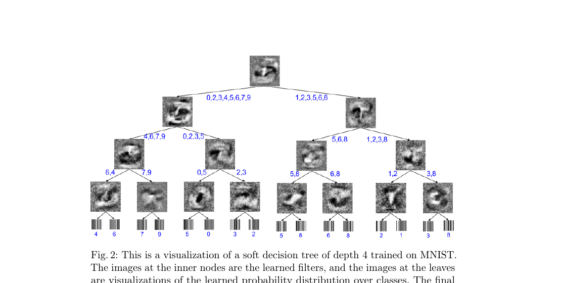
- Soft decision trees: distill a neural net into an interpretable tree. (Frosst & Hinton, 2017)
- TabNet: attention-based feature selection in a tree-like flow. (Arik & Pfister, AAAI 2021)
- NODE: differentiable oblivious tree ensembles, trained end-to-end. (Popov et al., ICLR 2020)
Summary
Non-parametric models let the data define structure, with few assumptions about functional form.
\(k\)-Nearest Neighbors: predict using nearby training points under a chosen distance metric.
\(k\)-Means: unsupervised grouping by distance, sensitive to initialization and the choice of \(k\).
Decision Trees: recursively split data into interpretable, flow-chart-like rules.
Ensembles: combine many simple models so their votes become stronger, more stable predictors.