
Lecture 6: Reinforcement Learning (Cont'd)
Shen Shen
April 16, 2025
2:30pm, Room 32-144
Modeling with Machine Learning for Computer Science
Outline
- Recap: Value iteration
- Tabular Q-learning
- Fitted/deep Q-learning
- Policy-based methods
- High-level idea
- Policy gradient
Last time, we ended at:
Value Iteration
- for \(s \in \mathcal{S}, a \in \mathcal{A}\) :
- \(\mathrm{Q}_{\text {old }}(\mathrm{s}, \mathrm{a})=0\)
- while True:
- for \(s \in \mathcal{S}, a \in \mathcal{A}\) :
- \(\mathrm{Q}_{\text {new }}(s, a) \leftarrow \mathrm{R}(s, a)+\gamma \sum_{s^{\prime}} \mathrm{T}\left(s, a, s^{\prime}\right) \max _{a^{\prime}} \mathrm{Q}_{\text {old }}\left(s^{\prime}, a^{\prime}\right)\)
- if \(\max _{s, a}\left|Q_{\text {old }}(s, a)-Q_{\text {new }}(s, a)\right|<\epsilon:\)
- return \(\mathrm{Q}_{\text {new }}\)
- \(\mathrm{Q}_{\text {old }} \leftarrow \mathrm{Q}_{\text {new }}\)
which gives us a recipe for finding \(\pi_h^*(s)\), by picking \(\arg \max _a \mathrm{Q}^h(s, a), \forall s, h\)
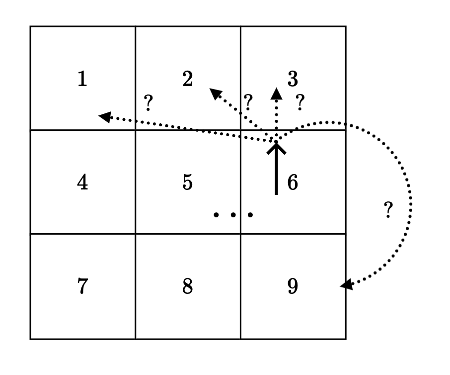
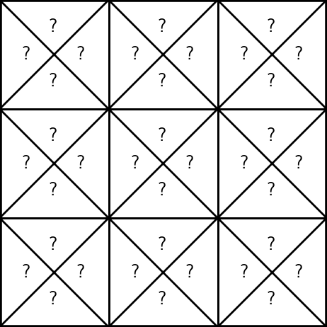
Recall:

\(\gamma = 0.9\)
States and one special transition:
- act optimally for one more timestep, at the next state \(s^{\prime}\)
- 20% chance, \(s'\) = 2, act optimally, receive \(\max _{a^{\prime}} \mathrm{Q}^{1}\left(2, a^{\prime}\right)\)
- 80% chance, \(s'\) = 3, act optimally, receive \(\max _{a^{\prime}} \mathrm{Q}^{1}\left(3, a^{\prime}\right)\)
\(= -10 + .9 [.2*0+ .8*1] = -9.28\)
- receive \(\mathrm{R}(6,\uparrow)\)
\(\mathrm{Q}^h(s, a)\): the expected sum of discounted rewards for
- starting in state \(s\),
- take action \(a\), for one step
- act optimally there afterwards for the remaining \((h-1)\) steps
Let's consider \(\mathrm{Q}^2(6, \uparrow) \)


\(=\mathrm{R}(6,\uparrow) + \gamma[.2 \max _{a^{\prime}} \mathrm{Q}^{1}\left(2, a^{\prime}\right)+ .8\max _{a^{\prime}} \mathrm{Q}^{1}\left(3, a^{\prime}\right)] \)
\(Q^2(6, \uparrow) =\mathrm{R}(6,\uparrow) + \gamma[.2 \max _{a^{\prime}} Q^{1}\left(2, a^{\prime}\right)+ .8\max _{a^{\prime}} Q^{1}\left(3, a^{\prime}\right)] \)
in general
Recall:
\(\gamma = 0.9\)
States and one special transition:
\(Q^h(s, a)\): the expected sum of discounted rewards for
- starting in state \(s\),
- take action \(a\), for one step
- act optimally there afterwards for the remaining \((h-1)\) steps
Outline
- Recap: Value iteration
- Tabular Q-learning
- Fitted/deep Q-learning
- Policy-based methods
- High-level idea
- Policy gradient
- Value iteration relied on having full access to \(\mathrm{R}\) and \(\mathrm{T}\)
- Without \(\mathrm{R}\) and \(\mathrm{T}\), how about we approximate like so:
- pick an \((s,a)\) pair
- execute \((s,a)\)
- observe \(r\) and \(s'\)
- update:
target
States and unknown transition:
Game Set up
Try using
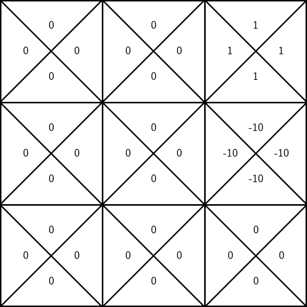
unknown rewards:
execute \((3, \uparrow)\), observe a reward \(r=1\)
\(\mathrm{Q}_\text{old}(s, a)\)
\(\mathrm{Q}_{\text{new}}(s, a)\)
States and unknown transition:
Try out
- execute \((6, \uparrow)\)
- update \(\mathrm{Q}(6, \uparrow)\) as:
\(-10 + 0.9 \max _{a^{\prime}} \mathrm{Q}_{\text {old }}\left(3, a^{\prime}\right)\)
= -10 + 0.9 = -9.1
To update the estimate of \(\mathrm{Q}(6, \uparrow)\):
- suppose, we observe a reward \(r=-10\), the next state \(s'=3\)
\(\gamma = 0.9\)
\(\mathrm{Q}_\text{old}(s, a)\)
\(\mathrm{Q}_{\text{new}}(s, a)\)
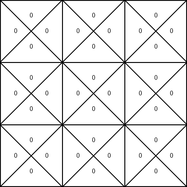
States and unknown transition:
- execute \((6, \uparrow)\) again
- update \(\mathrm{Q}(6, \uparrow)\) as:
\(-10 + 0.9 \max _{a^{\prime}} \mathrm{Q}_{\text {old }}\left(2, a^{\prime}\right)\)
= -10 + 0 = -10
- suppose, we observe a reward \(r=-10\), the next state \(s'=2\)
\(\gamma = 0.9\)
Try out
\(\mathrm{Q}_\text{old}(s, a)\)
\(\mathrm{Q}_{\text{new}}(s, a)\)
To update the estimate of \(\mathrm{Q}(6, \uparrow)\):

States and unknown transition:
Try out
- execute \((6, \uparrow)\) again
- update \(\mathrm{Q}(6, \uparrow)\) as:
\(-10 + 0.9 \max _{a^{\prime}} \mathrm{Q}_{\text {old }}\left(3, a^{\prime}\right)\)
= -10 + 0.9 = -9.1
To update the estimate of \(\mathrm{Q}(6, \uparrow)\):
- suppose, we observe a reward \(r=-10\), the next state \(s'=3\)
\(\gamma = 0.9\)
\(\mathrm{Q}_\text{old}(s, a)\)
\(\mathrm{Q}_{\text{new}}(s, a)\)
States and unknown transition:
- execute \((6, \uparrow)\) again
- update \(\mathrm{Q}(6, \uparrow)\) as:
\(-10 + 0.9 \max _{a^{\prime}} \mathrm{Q}_{\text {old }}\left(2, a^{\prime}\right)\)
= -10 + 0 = -10
- suppose, we observe a reward \(r=-10\), the next state \(s'=2\)
\(\gamma = 0.9\)
Try out
\(\mathrm{Q}_\text{old}(s, a)\)
\(\mathrm{Q}_{\text{new}}(s, a)\)
To update the estimate of \(\mathrm{Q}(6, \uparrow)\):
States and unknown transition:
Try out
- execute \((6, \uparrow)\) again
- update \(\mathrm{Q}(6, \uparrow)\) as:
\(-10 + 0.9 \max _{a^{\prime}} \mathrm{Q}_{\text {old }}\left(3, a^{\prime}\right)\)
= -10 + 0.9 = -9.1
To update the estimate of \(\mathrm{Q}(6, \uparrow)\):
- suppose, we observe a reward \(r=-10\), the next state \(s'=3\)
\(\gamma = 0.9\)
\(\mathrm{Q}_\text{old}(s, a)\)
\(\mathrm{Q}_{\text{new}}(s, a)\)
- Indeed, value iteration relied on having full access to \(\mathrm{R}\) and \(\mathrm{T}\)
- Without \(\mathrm{R}\) and \(\mathrm{T}\), perhaps we could execute \((s,a)\), observe \(r\) and \(s'\), and use
- But target keeps "washing away" the old progress.
target
🥺
- Indeed, value iteration relied on having full access to \(\mathrm{R}\) and \(\mathrm{T}\)
- Without \(\mathrm{R}\) and \(\mathrm{T}\), perhaps we could execute \((s,a)\), observe \(r\) and \(s'\), and use
old belief
learning rate
😍
- Amazingly, this way has nice convergence properties.
target
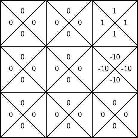
- execute \((6, \uparrow)\)
- update \(\mathrm{Q}(6, \uparrow)\) as:
\((-10 + \)
= -5 + 0.5(-10 + 0.9)= - 9.55
- suppose, we observe a reward \(r=-10\), the next state \(s'=3\)
States and unknown transition:
Better idea:
\(\gamma = 0.9\)
pick learning rate \(\alpha =0.5\)
+ 0.5
(1-0.5) * -10
\(\mathrm{Q}_\text{old}(s, a)\)
\(\mathrm{Q}_{\text{new}}(s, a)\)
To update the estimate of \(\mathrm{Q}(6, \uparrow)\):
\(0.9 \max _{a^{\prime}} \mathrm{Q}_{\text {old }}\left(3, a^{\prime}\right))\)
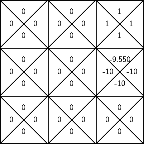
- execute \((6, \uparrow)\) again
\((-10\)
= 0.5*-9.55 + 0.5(-10 + 0)= -9.775
- suppose, we observe a reward \(r=-10\), the next state \(s'=2\)
States and unknown transition:
Better idea:
\(\gamma = 0.9\)
pick learning rate \(\alpha =0.5\)
+ 0.5
(1-0.5) * -9.55
\(\mathrm{Q}_\text{old}(s, a)\)
\(\mathrm{Q}_{\text{new}}(s, a)\)
To update the estimate of \(\mathrm{Q}(6, \uparrow)\):
- update \(\mathrm{Q}(6, \uparrow)\) as:
\(+ 0.9 \max _{a^{\prime}} \mathrm{Q}_{\text {old }}\left(2, a^{\prime}\right))\)
- for \(s \in \mathcal{S}, a \in \mathcal{A}\) :
- \(\mathrm{Q}_{\text {old }}(\mathrm{s}, \mathrm{a})=0\)
- while True:
- for \(s \in \mathcal{S}, a \in \mathcal{A}\) :
- \(\mathrm{Q}_{\text {new }}(s, a) \leftarrow \mathrm{R}(s, a)+\gamma \sum_{s^{\prime}} \mathrm{T}\left(s, a, s^{\prime}\right) \max _{a^{\prime}} \mathrm{Q}_{\text {old }}\left(s^{\prime}, a^{\prime}\right)\)
- if \(\max _{s, a}\left|Q_{\text {old }}(s, a)-Q_{\text {new }}(s, a)\right|<\epsilon:\)
- return \(\mathrm{Q}_{\text {new }}\)
- \(\mathrm{Q}_{\text {old }} \leftarrow \mathrm{Q}_{\text {new }}\)
Value Iteration\((\mathcal{S}, \mathcal{A}, \mathrm{T}, \mathrm{R}, \gamma, \epsilon)\)
"calculating"
"learning" (estimating)
Q-Learning \(\left(\mathcal{S}, \mathcal{A}, \gamma, \alpha, s_0\right. \text{max-iter})\)
1. \(i=0\)
2. for \(s \in \mathcal{S}, a \in \mathcal{A}:\)
3. \({\mathrm{Q}_\text{old}}(s, a) = 0\)
4. \(s \leftarrow s_0\)
5. while \(i < \text{max-iter}:\)
6. \(a \gets \text{select}\_\text{action}(s, {\mathrm{Q}_\text{old}}(s, a))\)
7. \(r,s' \gets \text{execute}(a)\)
8. \({\mathrm{Q}}_{\text{new}}(s, a) \leftarrow (1-\alpha){\mathrm{Q}}_{\text{old}}(s, a) + \alpha(r + \gamma \max_{a'}{\mathrm{Q}}_{\text{old}}(s', a'))\)
9. \(s \leftarrow s'\)
10. \(i \leftarrow (i+1)\)
11. \(\mathrm{Q}_{\text{old}} \leftarrow \mathrm{Q}_{\text{new}}\)
12. return \(\mathrm{Q}_{\text{new}}\)
"learning"
Q-Learning \(\left(\mathcal{S}, \mathcal{A}, \gamma, \alpha, s_0\right. \text{max-iter})\)
1. \(i=0\)
2. for \(s \in \mathcal{S}, a \in \mathcal{A}:\)
3. \({\mathrm{Q}_\text{old}}(s, a) = 0\)
4. \(s \leftarrow s_0\)
5. while \(i < \text{max-iter}:\)
6. \(a \gets \text{select}\_\text{action}(s, {\mathrm{Q}_\text{old}}(s, a))\)
7. \(r,s' \gets \text{execute}(a)\)
8. \({\mathrm{Q}}_{\text{new}}(s, a) \leftarrow (1-\alpha){\mathrm{Q}}_{\text{old}}(s, a) + \alpha(r + \gamma \max_{a'}{\mathrm{Q}}_{\text{old}}(s', a'))\)
9. \(s \leftarrow s'\)
10. \(i \leftarrow (i+1)\)
11. \(\mathrm{Q}_{\text{old}} \leftarrow \mathrm{Q}_{\text{new}}\)
12. return \(\mathrm{Q}_{\text{new}}\)
- Remarkably, 👈 can converge to the true infinite-horizon Q-values\(^1\).
\(^1\) given we visit all \(s,a\) infinitely often, and satisfy a condition on the learning rate \(\alpha\).
- But the convergence can be extremely slow.
- During learning, especially in early stages, we'd like to explore, and observe diverse \((s,a\)) consequences.
- \(\epsilon\)-greedy action selection strategy:
- with probability \(\epsilon\), choose an action \(a \in \mathcal{A}\) uniformly at random
- with probability \(1-\epsilon\), choose \(\arg \max _{\mathrm{a}} \mathrm{Q}_{\text{old}}(s, \mathrm{a})\)
- \(\epsilon\) controls the trade-off between exploration vs. exploitation.
the current estimate of \(\mathrm{Q}\) values
"learning"
Q-Learning \(\left(\mathcal{S}, \mathcal{A}, \gamma, \alpha, s_0\right. \text{max-iter})\)
1. \(i=0\)
2. for \(s \in \mathcal{S}, a \in \mathcal{A}:\)
3. \({\mathrm{Q}_\text{old}}(s, a) = 0\)
4. \(s \leftarrow s_0\)
5. while \(i < \text{max-iter}:\)
6. \(a \gets \text{select}\_\text{action}(s, {\mathrm{Q}_\text{old}}(s, a))\)
7. \(r,s' \gets \text{execute}(a)\)
8. \({\mathrm{Q}}_{\text{new}}(s, a) \leftarrow (1-\alpha){\mathrm{Q}}_{\text{old}}(s, a) + \alpha(r + \gamma \max_{a'}{\mathrm{Q}}_{\text{old}}(s', a'))\)
9. \(s \leftarrow s'\)
10. \(i \leftarrow (i+1)\)
11. \(\mathrm{Q}_{\text{old}} \leftarrow \mathrm{Q}_{\text{new}}\)
12. return \(\mathrm{Q}_{\text{new}}\)
Outline
- Recap: Value iteration
- Tabular Q-learning
- Fitted/deep Q-learning
- Policy-based methods
- High-level idea
- Policy gradient
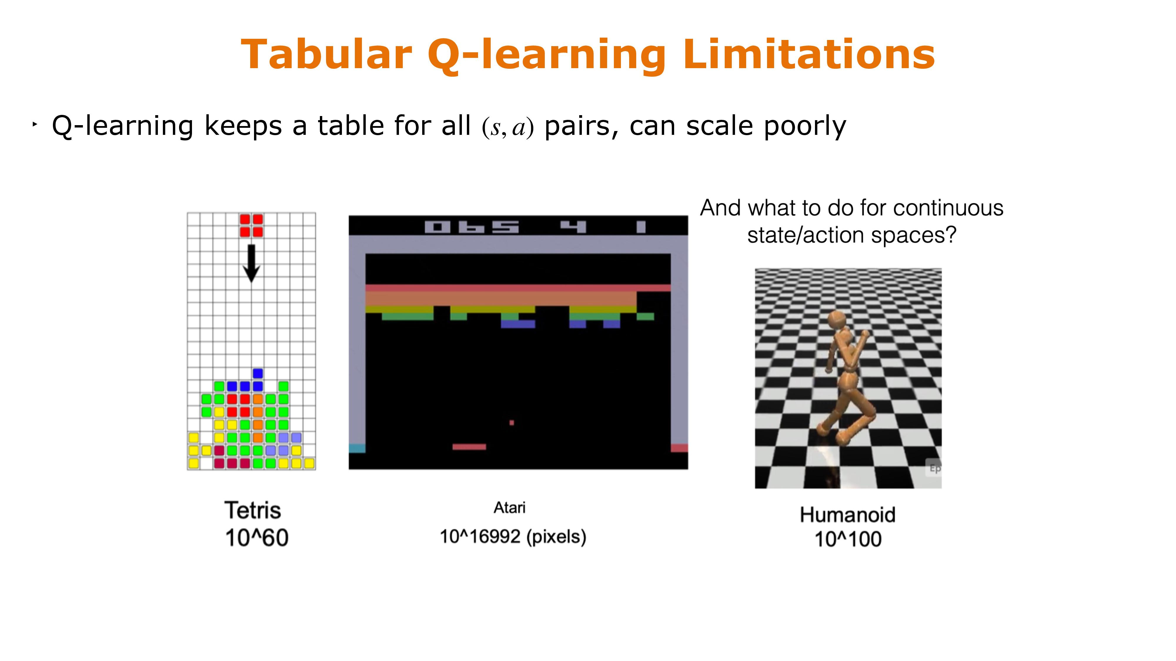
Tabular Q-learning limitations
- What do we do if \(\mathcal{S}\) and/or \(\mathcal{A}\) are large, or even continuous?
- Notice that the key update line in Q-learning algorithm:
is equivalently:
\(\mathrm{Q}_{\text {new}}(s, a) \leftarrow\mathrm{Q}_{\text {old }}(s, a)+\alpha\left([r+\gamma \max _{a^{\prime}} \mathrm{Q}_{\text {old}}(s', a')] - \mathrm{Q}_{\text {old }}(s, a)\right)\)
new belief
\(\leftarrow\)
old belief
learning rate
target
old belief
- Reminds us of: when minimizing \((\text{target} - \text{guess}_{\theta})^2\)
\(\mathrm{Q}_{\text {new}}(s, a) \leftarrow\mathrm{Q}_{\text {old }}(s, a)+\alpha\left([r+\gamma \max _{a^{\prime}} \mathrm{Q}_{\text {old}}(s', a')] - \mathrm{Q}_{\text {old }}(s, a)\right)\)
new belief
\(\leftarrow\)
old belief
learning rate
target
old belief
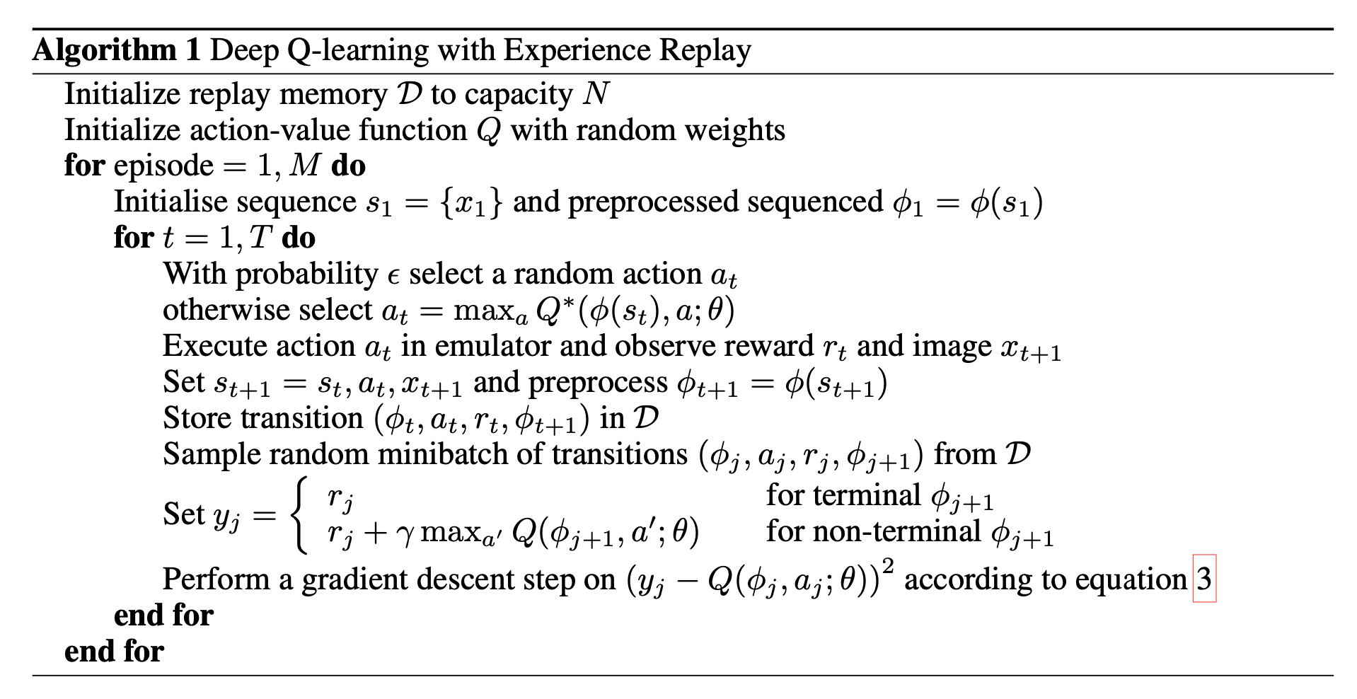
- Generalize tabular Q-learning for continuous state/action space:
\(\left(\mathrm{Q}_{\theta}(s, a)-\text{target}\right)^2\)
Gradient descent does: \(\theta_{\text{new}} \leftarrow \theta_{\text{old}} + \eta (\text{target} - \text{guess}_{\theta})\frac{\nabla \text{guess}}{\nabla \theta}\)
- parameterize \(\mathrm{Q}_{\theta}(s,a)\)
- collect data \((r, s')\) to construct the target
- update \(\theta\) via gradient-descent methods to minimize
\(r+\gamma \max _{a^{\prime}} \mathrm{Q}_{\theta}\left(s^{\prime}, a^{\prime}\right)\)
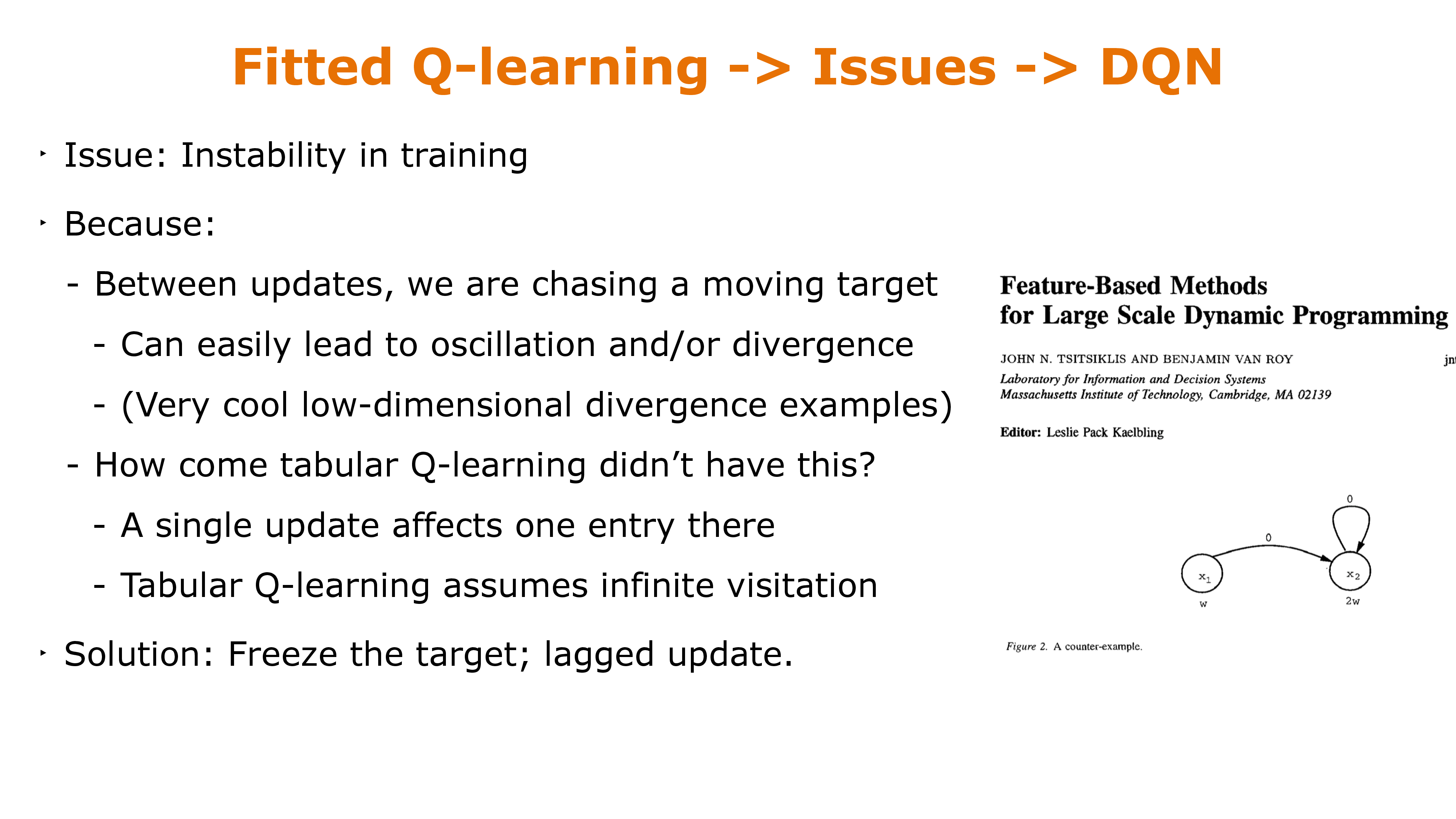
Fitted Q-learning limitations
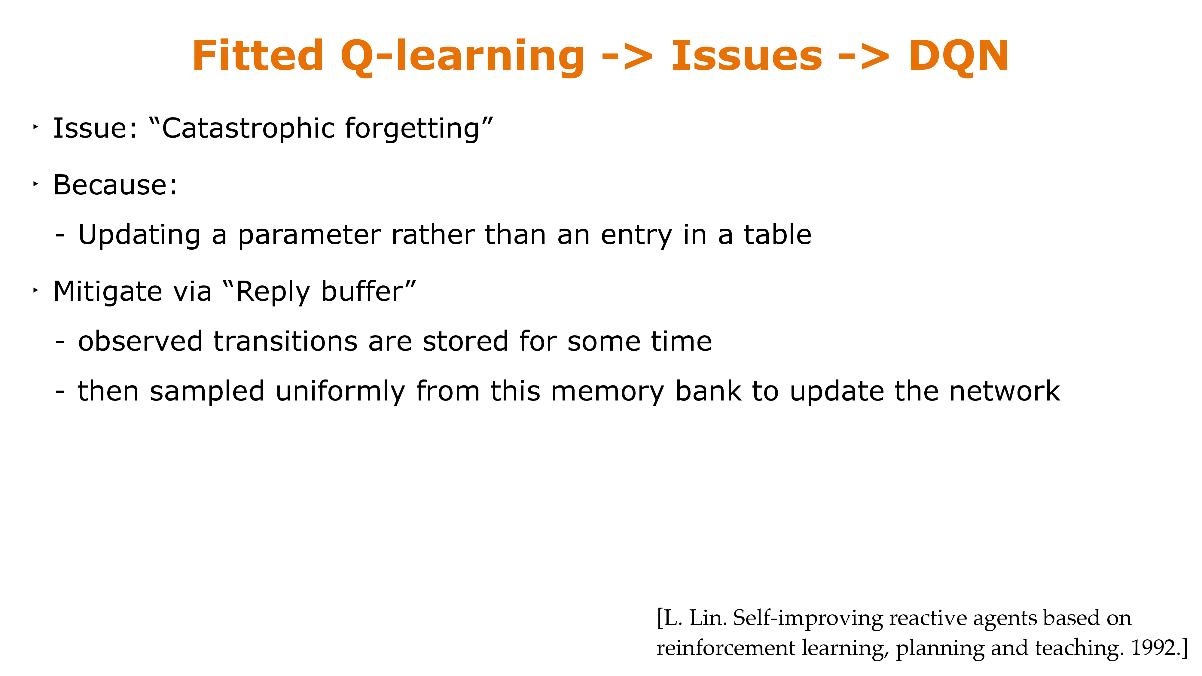
Q-learning limitations
Fitted Q-learning limitations

General value-based method limitations
Quick Summary
- In reinforcement learning, we assume we are interacting with an unknown MDP, but we still want to find a good policy. We will do so via estimating the Q value function.
- One problem is how to select actions to gain good reward while learning. This “exploration vs exploitation” problem is important.
- Q-learning, for discrete-state problems, will converge to the optimal value function (with enough exploration).
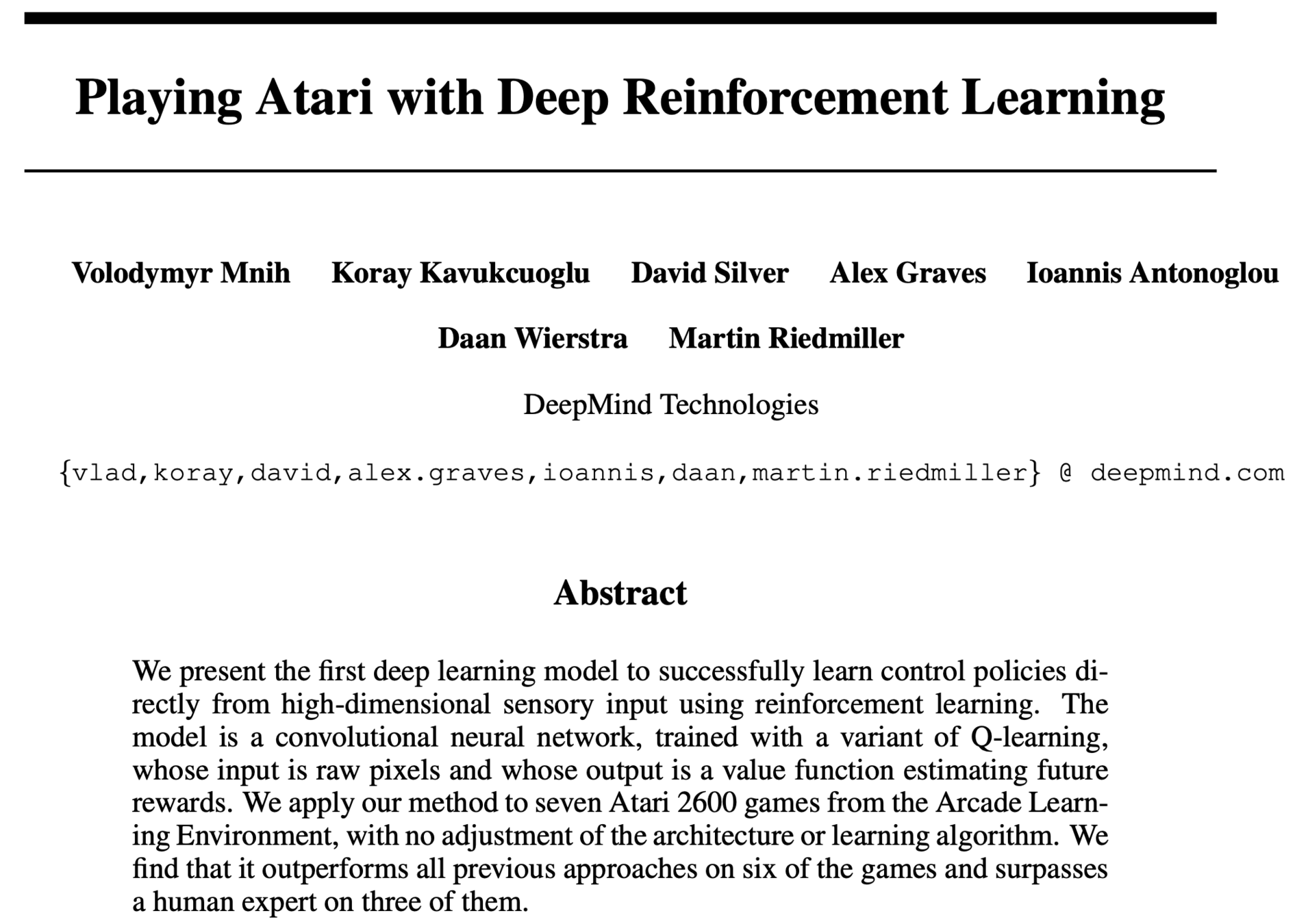
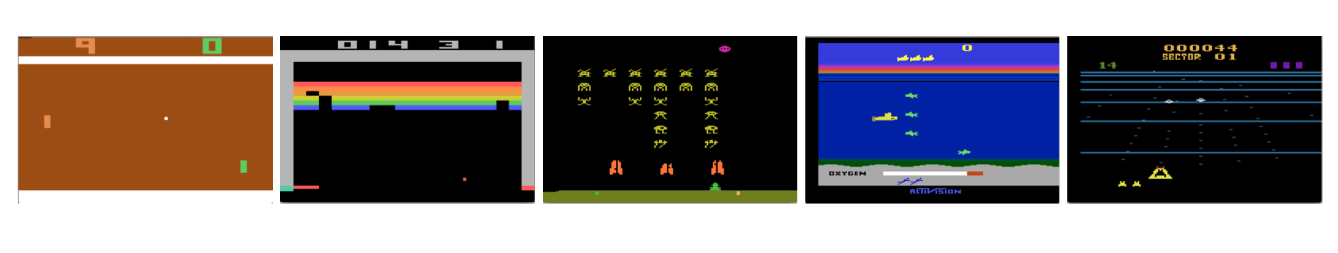
- “Deep Q learning” can be applied to continuous-state or large discrete-state problems by using a parameterized function to represent the Q-values.
Outline
- Recap: Value iteration
- Tabular Q-learning
- Fitted/deep Q-learning
-
Policy-based methods
- High-level idea
- Policy gradient
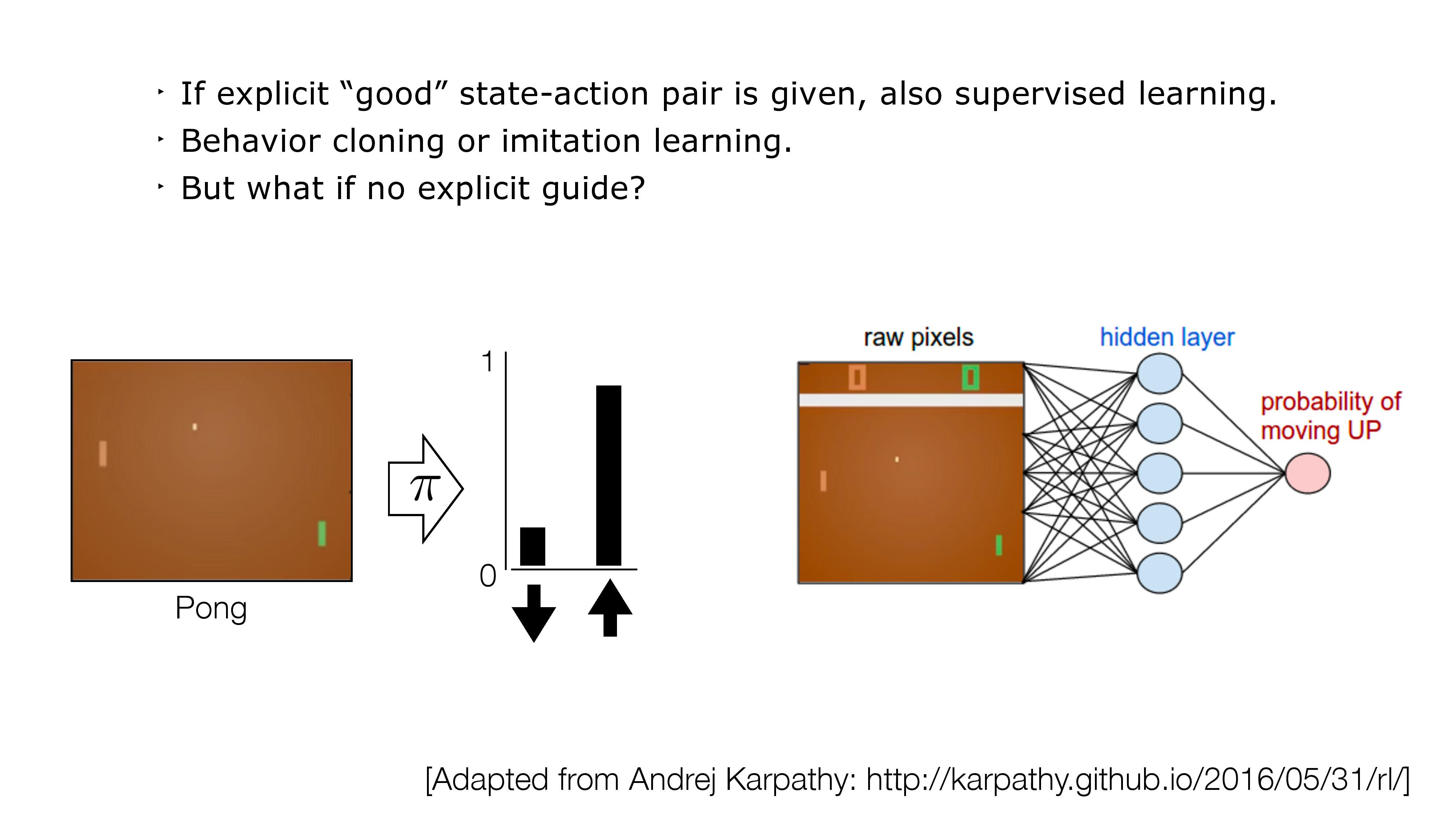
- Often \(\pi\) can be simpler than \(Q\) or \(V\)
- e.g. lots of \(\pi\) are roughly good
- \(V(s)\) : doesn't prescribe actions
- Q: need to be able to efficiently solve \(\arg \max_a Q(s, a)\), can also be challenging for continuous / high-dimensional action spaces
- Maybe makes sense to direct optimize policy end-to-end
- So how do we do this?
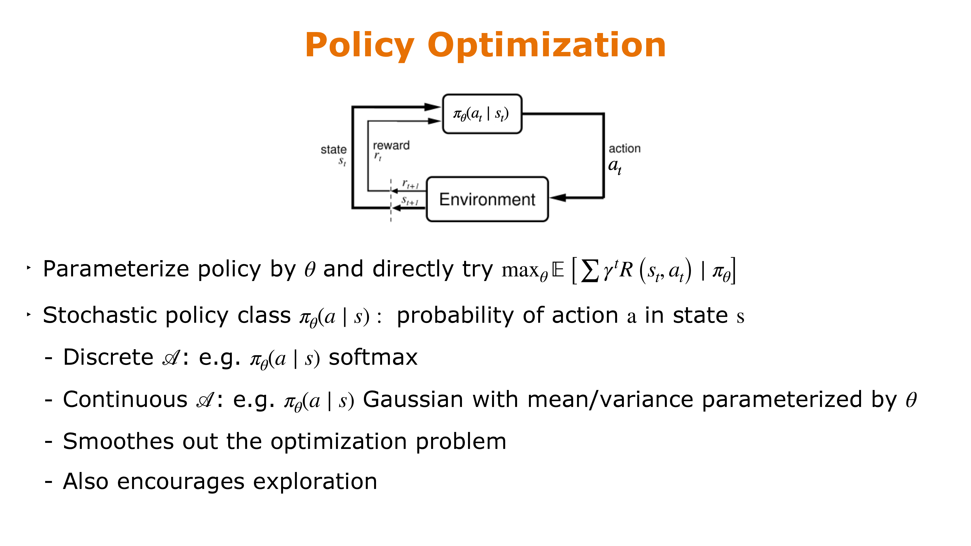
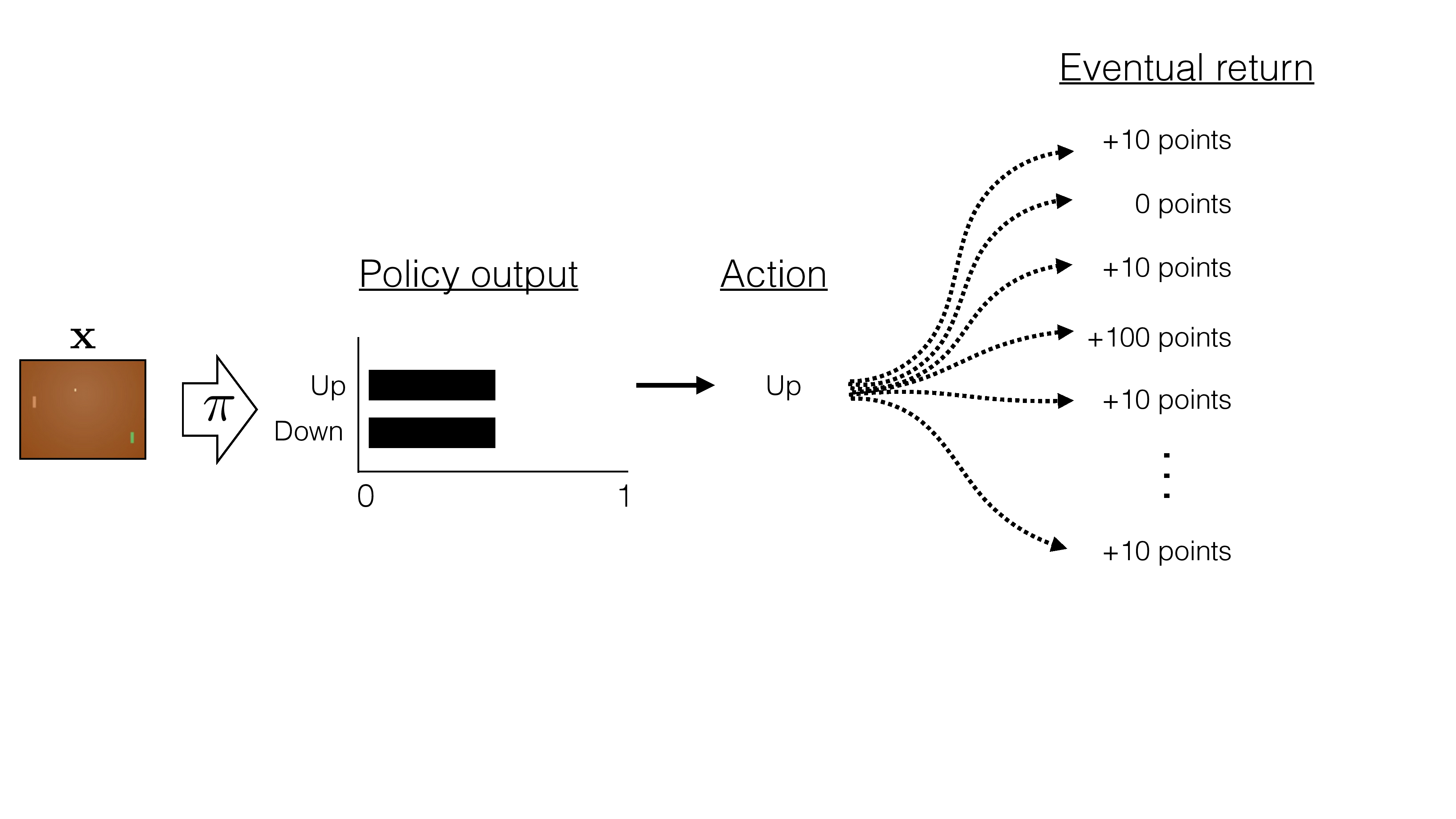
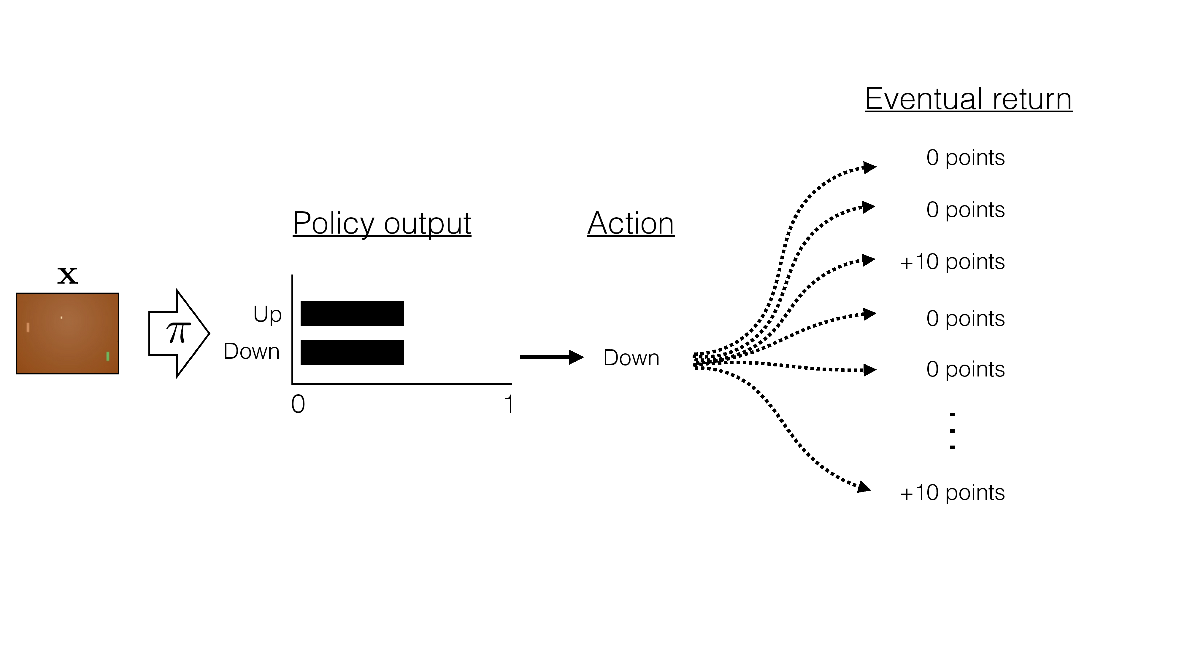
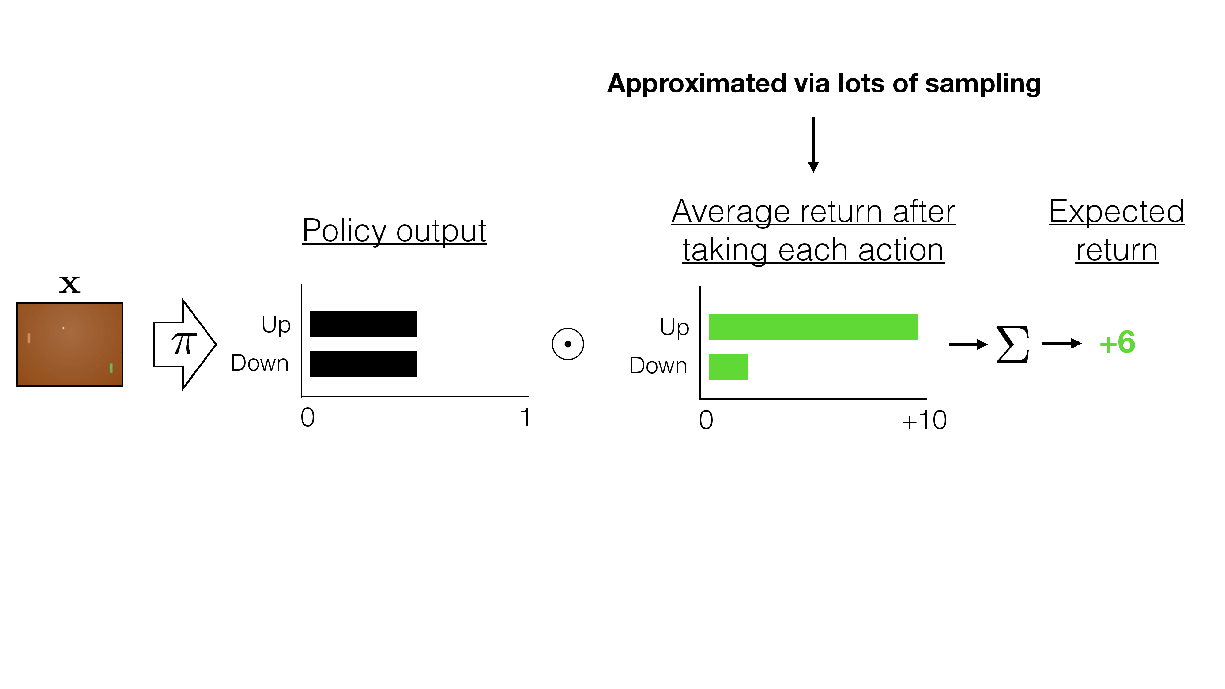
- Parameterize policy by \(\theta\) and directly try \(\max _\theta \mathbb{E}\left[\sum \gamma^t R\left(s_t, a_t\right) \mid \pi_\theta\right]\)
- Stochastic policy class \(\pi_\theta(a \mid s)\) : probability of action a in state s
- Discrete \(\mathcal{A}\) : e.g. \(\pi_\theta(a \mid s)\) softmax
- Continuous \(\mathcal{A}\) : e.g. \(\pi_\theta(a \mid s)\) Gaussian with mean/variance parameterized by \(\theta\)
- Smoothes out the optimization problem
- Also encourages exploration
Outline
- Recap: Value iteration
- Tabular Q-learning
- Fitted/deep Q-learning
- Policy-based methods
- High-level idea
- Policy gradient
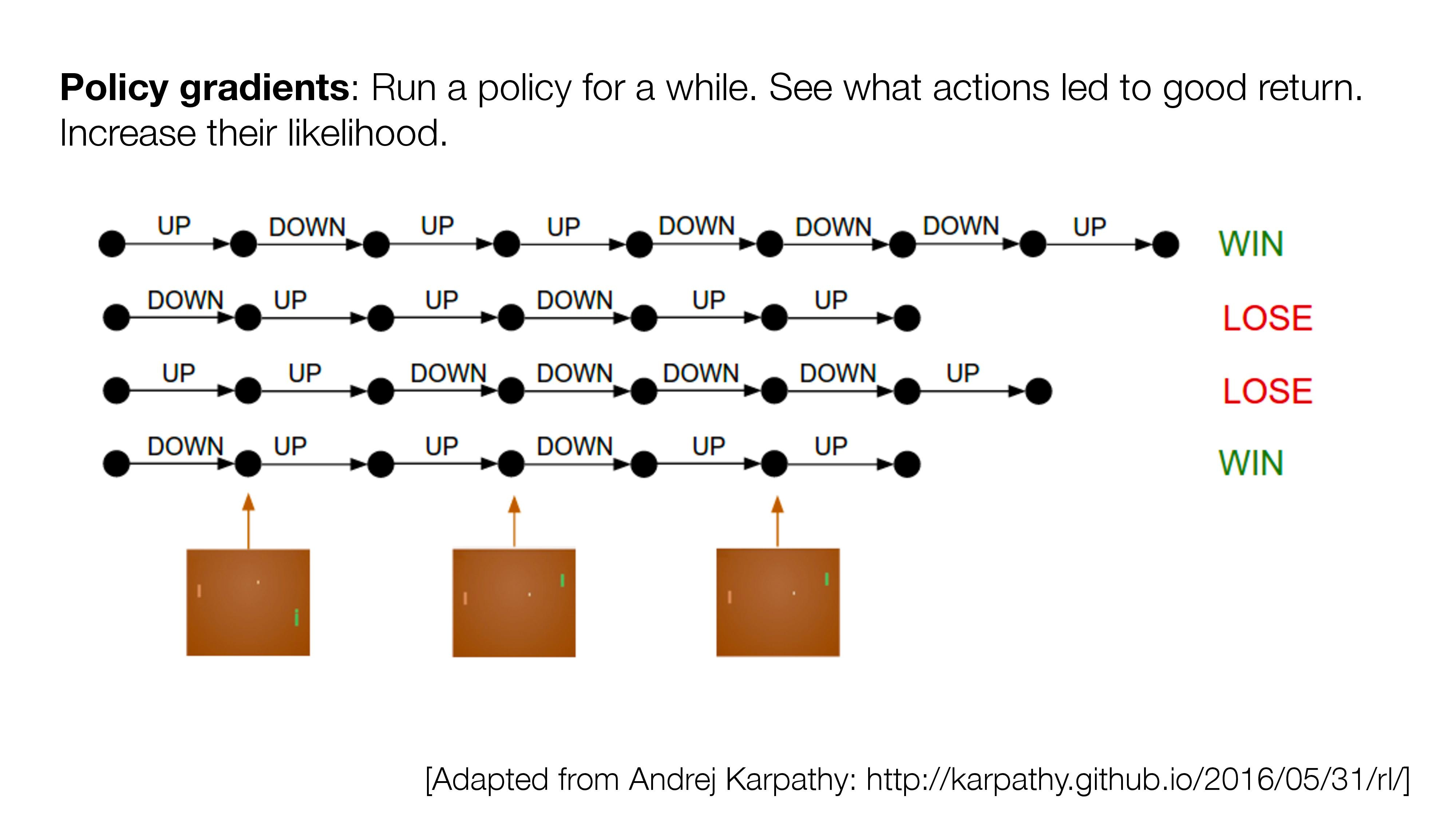
Policy Gradient Derivation
- We overload notation:
- Let \(\tau\) denote a state-action sequence: \(\tau=s_0, a_0, s_1, a_1, \ldots\)
- Let \(R(\tau)\) denote the sum of discounted rewards on \(\tau: R(\tau)=\sum_t \gamma^t R\left(s_t, a_t\right)\)
- W.l.o.g. assume \(R(\tau)\) is deterministic in \(\tau\)
- Let \(P(\tau ; \theta)\) denote the probability of trajectory \(\tau\) induced by \(\pi_\theta\)
- Let \(U(\theta)\) denote the objective: \(U(\theta)=\mathbb{E}\left[\sum_t \gamma^t R\left(s_t, a_t\right) \mid \pi_\theta\right]\)
- Our goal is to find \[\theta: \max _\theta U(\theta)=\max _\theta \sum_\tau P(\tau ; \theta) R(\tau)\]
Policy Gradient Derivation
Identity \(\begin{aligned} \nabla_\theta p_\theta(\tau) & =p_\theta(\tau) \frac{\nabla_\theta p_\theta(\tau)}{p_\theta(\tau)} \\ & =p_\theta(\tau) \nabla_\theta \log p_\theta(\tau)\end{aligned}\)
\(=\nabla_\theta \sum_\tau P(\tau ; \theta) R(\tau)\)
\(=\sum_\tau \nabla_\theta P(\tau ; \theta) R(\tau)\)
\(=\sum_\tau \frac{P(\tau ; \theta)}{P(\tau ; \theta)} \nabla_\theta P(\tau ; \theta) R(\tau)\)
\(=\sum_\tau P(\tau ; \theta) \frac{\nabla_\theta P(\tau ; \theta)}{P(\tau ; \theta)} R(\tau)\)
\(=\sum_\tau P(\tau ; \theta) \nabla_\theta \log P(\tau ; \theta) R(\tau)\)
\(\nabla_\theta U(\theta)\)
Policy Gradient Derivation
where \(P(\tau ; \theta)=\prod_{t=0} \underbrace{P\left(s_{t+1} \mid s_t, a_t\right)}_{\text {transition }} \cdot \underbrace{\left.\pi_\theta\left(a_t \mid s_t\right)\right]}_{\text {policy }}\)
\(=\sum_\tau P(\tau ; \theta) \nabla_\theta \log P(\tau ; \theta) R(\tau)\)
\(\nabla_\theta U(\theta)\)
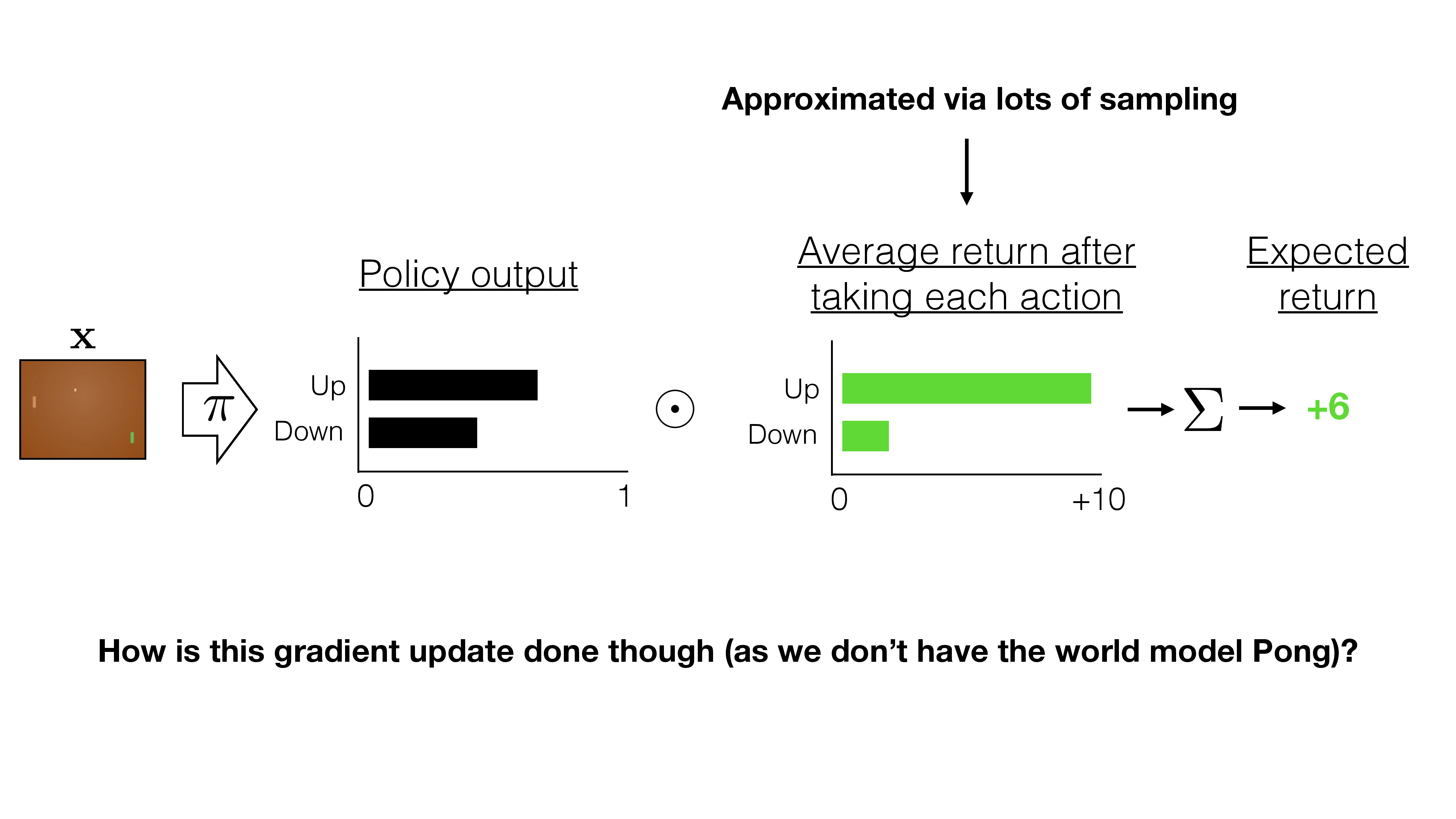
Transition is unknown....
Stuck?
Policy Gradient Derivation
\(=\sum_\tau P(\tau ; \theta) \nabla_\theta \log P(\tau ; \theta) R(\tau)\)
\(\nabla_\theta U(\theta)\)
Approximate with the empirical estimate for \(m\) sample traj. under policy \(\pi_\theta\)
\(\nabla_\theta U(\theta) \approx \hat{g}=\frac{1}{m} \sum_{i=1}^m \nabla_\theta \log P\left(\tau^{(i)} ; \theta\right) R\left(\tau^{(i)}\right)\)
Valid even when:
- Reward function discontinuous and/or unknown
- Discrete state and/or action spaces
Policy Gradient Derivation
where \(P(\tau ; \theta)=\prod_{t=0} \underbrace{P\left(s_{t+1} \mid s_t, a_t\right)}_{\text {transition }} \cdot \underbrace{\left.\pi_\theta\left(a_t \mid s_t\right)\right]}_{\text {policy }}\)
\(=\nabla_\theta \log [\prod_{t=0} \underbrace{P\left(s_{t+1} \mid s_t, a_t\right)}_{\text {transition }} \cdot \underbrace{\left.\pi_\theta\left(a_t \mid s_t\right)\right]}_{\text {policy }}\)
\(=\nabla_\theta\left[\sum_{t=0} \log P\left(s_{t+1} \mid s_t, a_t\right)+\sum_{t=0} \log \pi_\theta\left(a_t \mid s_t\right)\right]\)
\(=\nabla_\theta \sum_{t=0} \log \pi_\theta\left(a_t \mid s_t\right)\)
\(=\sum_{t=0} \underbrace{\nabla_\theta \log \pi_\theta\left(a_t \mid s_t\right)}_{\text {no transition model required, }}\)
\(\nabla_\theta \log P(\tau ; \theta)\)
\(\nabla_\theta U(\theta) \approx \hat{g}=\frac{1}{m} \sum_{i=1}^m \nabla_\theta \log P\left(\tau^{(i)} ; \theta\right) R\left(\tau^{(i)}\right)\)
Policy Gradient Derivation
\(=\sum_{t=0} \underbrace{\nabla_\theta \log \pi_\theta\left(a_t \mid s_t\right)}_{\text {no transition model required, }}\)
\(\nabla_\theta \log P(\tau ; \theta)\)
\(\nabla_\theta U(\theta) \approx \hat{g}=\frac{1}{m} \sum_{i=1}^m \nabla_\theta \log P\left(\tau^{(i)} ; \theta\right) R\left(\tau^{(i)}\right)\)
The following expression provides us with an unbiased estimate of the gradient, and we can compute it without access to the world model:

Unbiased estimator \(\mathrm{E}[\hat{g}]=\nabla_\theta U(\theta)\), but very noisy.
where
Thanks!
We'd love to hear your thoughts.