Topological Polymers and Random Embeddings of Graphs
/erice22
This talk!

Collaborators


Jason Cantarella
U. of Georgia
Tetsuo Deguchi
Ochanomizu U.
Erica Uehara
Ochanomizu U.
Funding: Simons Foundation (#524120, J.C.; #709150, C.S.), Japan Science and Technology Agency (CREST JPMJCR19T4, Deguchi Lab), Japan Society for the Promotion of Science (KAKENHI JP17H06463)
Equilibrium Distributions for Large Molecules
Want to define a probability distribution on the positions of \(\mathcal{V}\) points (i.e., monomers) in \(\mathbb{R}^3\).
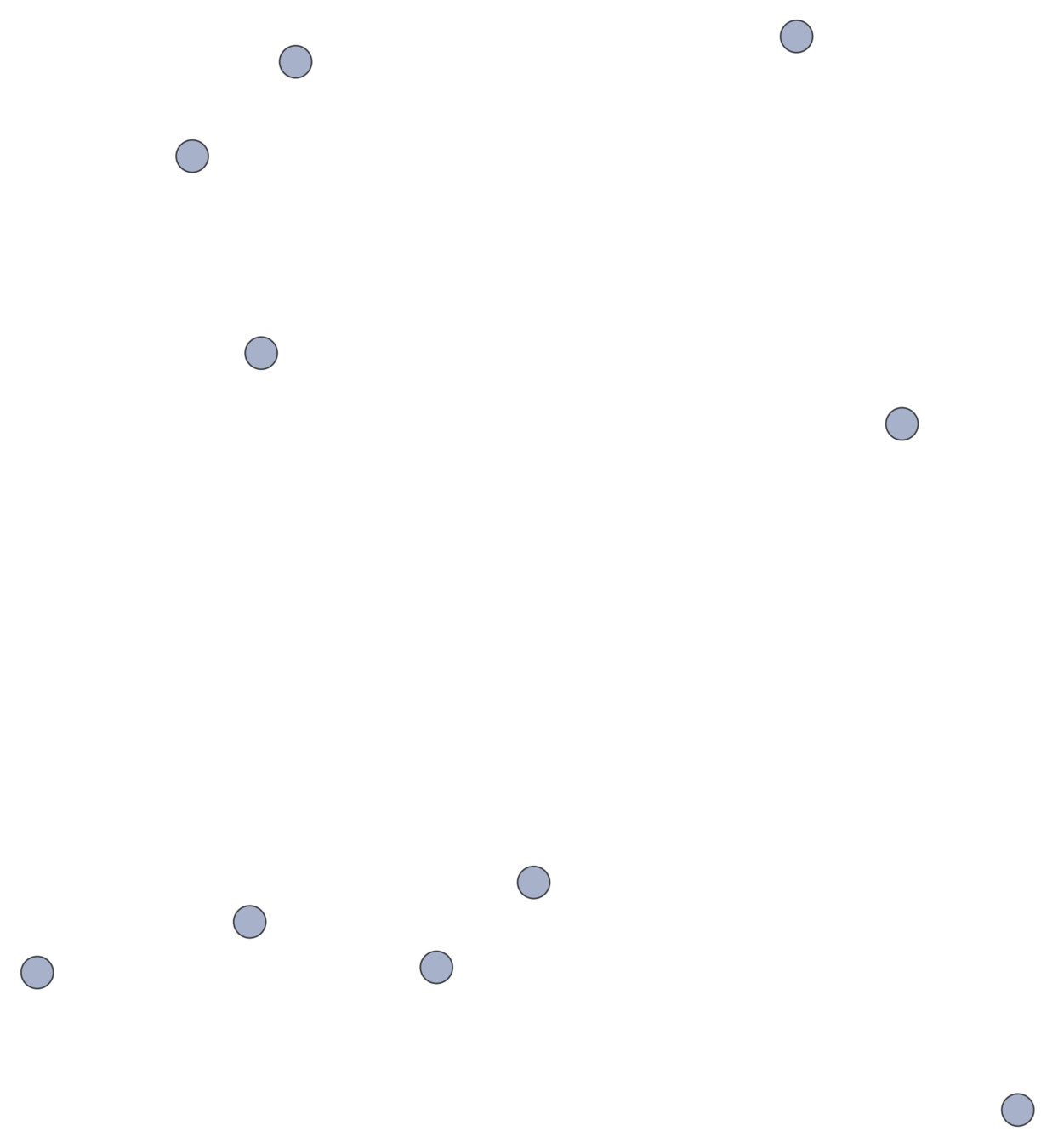
If positions are coupled (by a bond, steric effect, etc.), add an edge between points, forming a graph \(\mathcal{G}\).
Edge Distributions
Interactions are symmetric probability distributions on edge vectors.
Problem.
Edge vectors are not independent when there are loops.
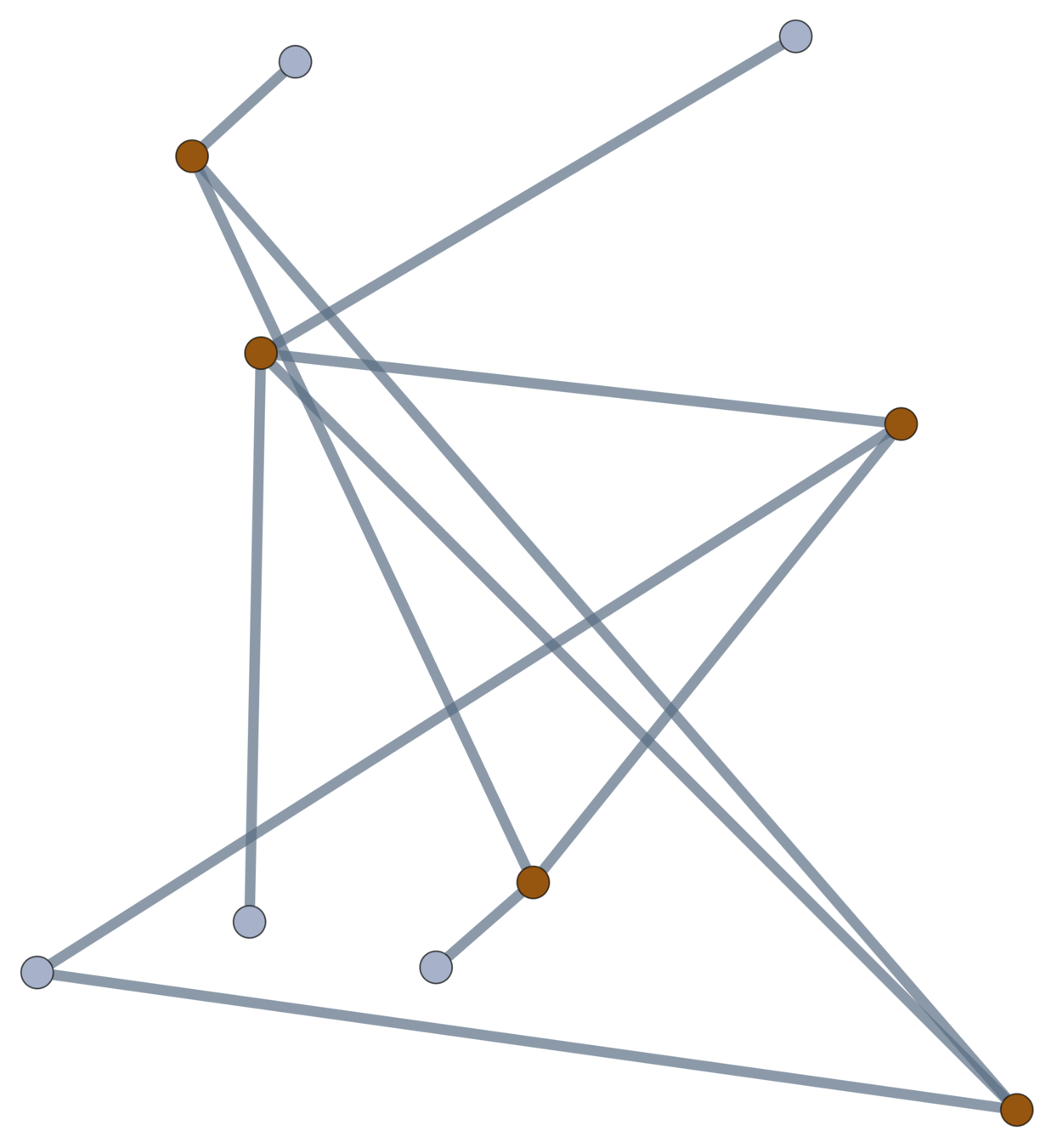
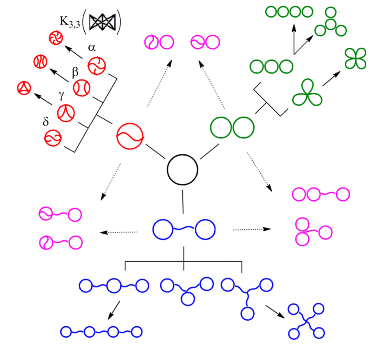
Topological Polymers
A topological polymer joins monomers in any (multi)graph type.
Chemistry Answer
Elasticity theory (1940s–1980s, James, Guth, Flory, Eichinger, etc.).

Structure graph \(\mathcal{G}\)
Edges i.i.d. Gaussian conditioned on \(\mathcal{G}\)
Theorem [Estrada–Hatano, James–Guth]
The expected variation size \(\mathbb{E}[\sum \|\delta p_i\|^2] = \frac{d}{\mathfrak{V}} \operatorname{tr}L^+\).
Theorem [Estrada–Hatano, James–Guth]
The expected variation size \(\mathbb{E}[\sum \|\delta p_i\|^2] = \frac{974299}{765600}\).
Theorem [Estrada–Hatano, James–Guth]
The expected variation size \(\mathbb{E}[\sum \|\delta p_i\|^2] = \frac{d}{\mathfrak{V}} \operatorname{tr}L^+\).
Graph Laplacian of \(\mathcal{G}\)
Theorem [Estrada–Hatano, James–Guth]
The expected variation size \(\mathbb{E}[\sum \|\delta p_i\|^2] = \frac{d}{\mathfrak{V}} \operatorname{tr}L^+\).
Our Approach
Problem.
Classical elasticity assumes mean-zero Gaussians. This assumption is built into the theory.
Solution.
New formalism which handles arbitrary distributions in a clean, provable way.
Classical Materials
Natural elastic materials tend to have extremely complicated, random graph types
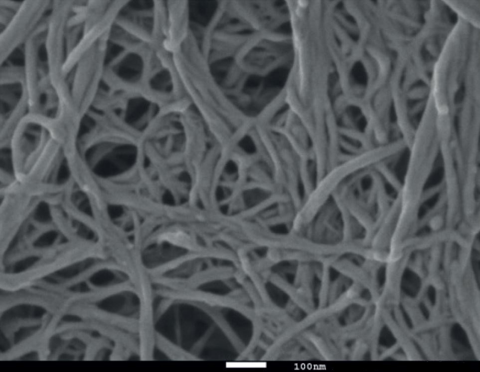
Wood-based nanofibrillated cellulose
Qspheroid4 [CC BY-SA 4.0], from Wikimedia Commons
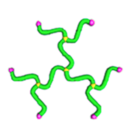
New Materials
Synthetic chemists can now produce simple topological polymers in usable quantities.
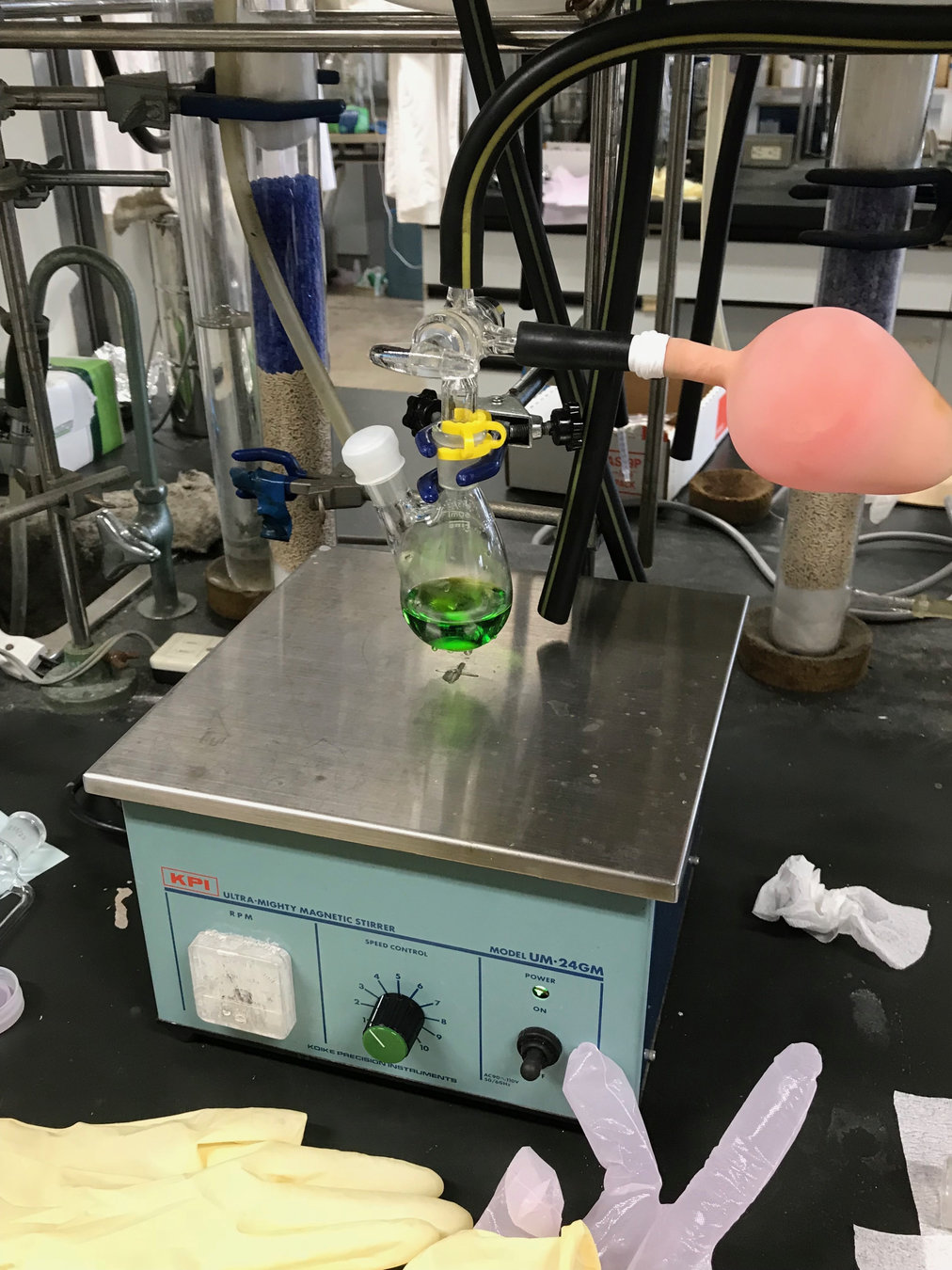
\(\theta\)-curves in solution at the Tezuka lab
Ansatz
Linear polymers
Topological polymers
Independently
Conditioned on graph type
Edges chosen from some \(O(d)\)-invariant distribution \(\mu\).
What does this mean?
Chain Groups
Let \(\mathcal{G}\) be a (directed) graph with \(\mathcal{E}\) edges and \(\mathcal{V}\) vertices.
Definition.
The vector space \(\operatorname{VC}\) of vertex chains is the vector space of (formal) linear combinations of vertices:
\(x = x_1 v_1 + \dots + x_{\mathcal{V}}v_{\mathcal{V}}\).
Definition.
The vector space \(\operatorname{EC}\) of edge chains is the vector space of (formal) linear combinations of edges:
\(w = w_1 e_1 + \dots + w_{\mathcal{E}}e_{\mathcal{E}}\).
Boundaries
Definition.
The boundary map \(\partial : \operatorname{EG} \to \operatorname{VC}\) is defined by
\(\partial(e_i) = \operatorname{head}(e_i) - \operatorname{tail}(e_i)\).

Definition.
\(\operatorname{ker} \partial \subset \operatorname{EC}\) is the loop space of \(\mathcal{G}\).

Boundaries
Definition.
Every \(w \in \ker \partial \subset \operatorname{EC}\) is a linear combination of closed loops. \(\dim\ker \partial\) is the cycle rank \(\xi(\mathcal{G}) = \mathcal{E} - \mathcal{V}+1\); i.e., the first Betti number of \(\mathcal{G}\).
\(\xi(\mathcal{G}) = \frac{1}{2} \sum_{i=1}^{\mathcal{V}} \left( \deg(v_i)-2\right) + 1\).
\(-\)
\(=\)
Embedding Spaces
The chain spaces encode the topology of the graph. The embedding into \(\mathbb{R}^d\) is determined by:
Definition.
The space of vertex positions \(\operatorname{VP} := \operatorname{Hom}(\operatorname{VC},\mathbb{R}^d)\).
Definition.
The space of edge displacements \(\operatorname{ED} = \operatorname{Hom}(\operatorname{EC},\mathbb{R}^d)\).
Definition.
The displacement map \(\operatorname{disp}: \operatorname{VP} \to \operatorname{ED}\) is given by
\(\operatorname{disp}(X)(e_i) = X(\operatorname{head}(e_i)) - X(\operatorname{tail}(e_i))\).
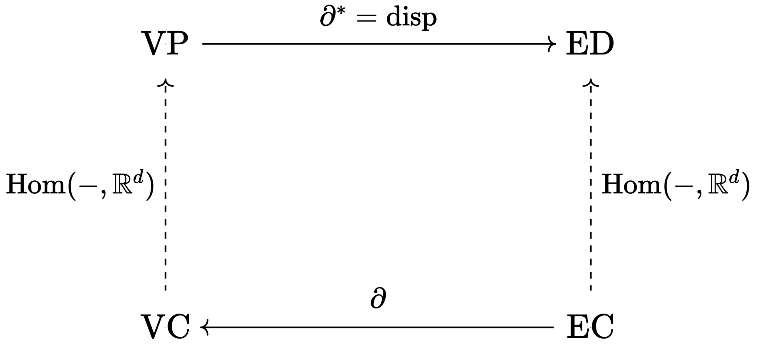
A Wild Functor Appears!
Proposition.
The map \(\operatorname{disp}:\operatorname{VP} \to \operatorname{ED}\) is equal to the map \(\partial^\ast\) induced by the contravariant functor \(\operatorname{Hom}(-,\mathbb{R}^d)\).
Proposition.
If \(\mathcal{G}\) is connected,
\(\operatorname{im}\partial^\ast = \{W \in \operatorname{ED} : W(u) = 0\) for all \(u \in \ker \partial\}\).
Random Graph Embeddings
Theorem.
The space of assignments of edge displacements compatible with the graph type \(\mathcal{G}\) is the linear subspace
\(\operatorname{im}\operatorname{disp} = \operatorname{im}\partial^\ast\).
Definition.
A probability measure \(\mu\) on \(\operatorname{ED}\) is admissible if it has finite first moment and is invariant under the diagonal action of \(O(d)\).
“A probability distribution on embeddings of \(\mathcal{G}\) is the restriction of an admissible probability measure \(\mu\) to the \(d(\mathcal{V}-1)\)-dimensional subspace \(\operatorname{im}\partial^\ast \subset \operatorname{ED}\).”
Gaussian Embeddings – Phantom Network Theory
Definition.
The distribution \(\mu\) on ED is the standard Gaussian; restriction to \(\operatorname{im}\partial^\ast\) is standard Gaussian on that subspace.
\(\operatorname{ED} \simeq \mathbb{R}^{3\mathcal{E}}\)
\(\operatorname{VP} \simeq \mathbb{R}^{3\mathcal{V}}\)
\(\partial^\ast\)
\(\operatorname{im}\partial^\ast\)
?
\(\partial^{\ast +}\)
\((\operatorname{ker}\partial^\ast)^\bot\)
The Correct Inner Product on VP
\((\operatorname{ED}, \langle\, , \,\rangle)\)
\((\operatorname{VP}, \langle \, , \, \rangle_{\widetilde{L}^\ast})\)
\(\partial^\ast\)
\(\operatorname{im}\partial^\ast\)
\(\partial^{\ast +}\)
\((\operatorname{ker}\partial^\ast)^\bot\)
Definition.
The graph Laplacian \(L: \operatorname{VC} \to \operatorname{VC}\) is \(L:=\partial \partial^T\).
Proposition.
With the inner product \(\langle X, Y \rangle_{\widetilde{L}^\ast} = \langle X, \widetilde{L}^\ast Y \rangle\) on VP, \(\partial^\ast\) and \(\partial^{\ast +}\) are partial isometries.
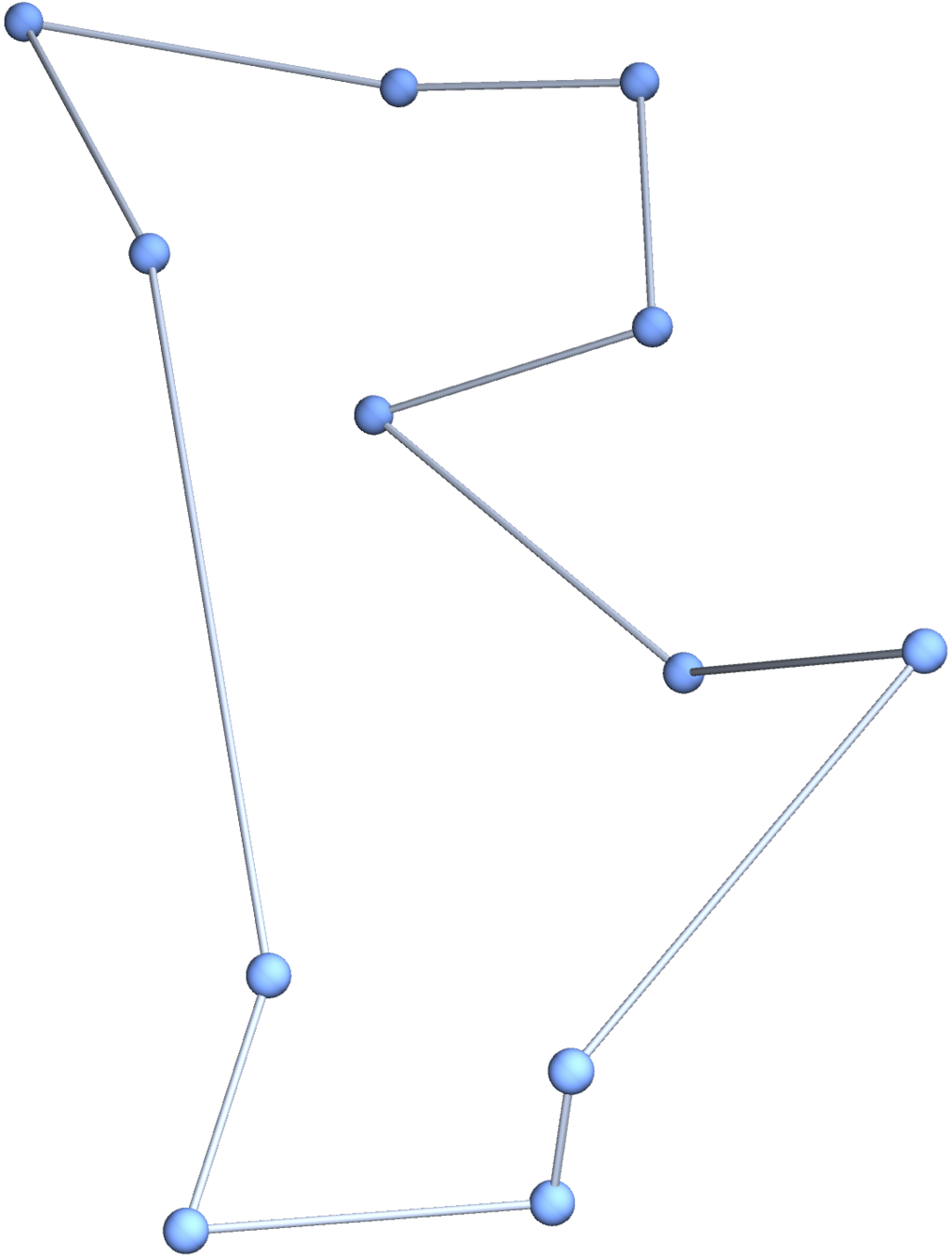
Sampling
- Compute pseudoinverse \(\partial^{\ast +}: \operatorname{ED} \to \operatorname{VP}\).
- Sample \(W\) from conditional distribution on \(\operatorname{im}\partial^\ast \subset \operatorname{ED}\).
- Construct vertex positions \(X = \partial^{\ast +} W\).
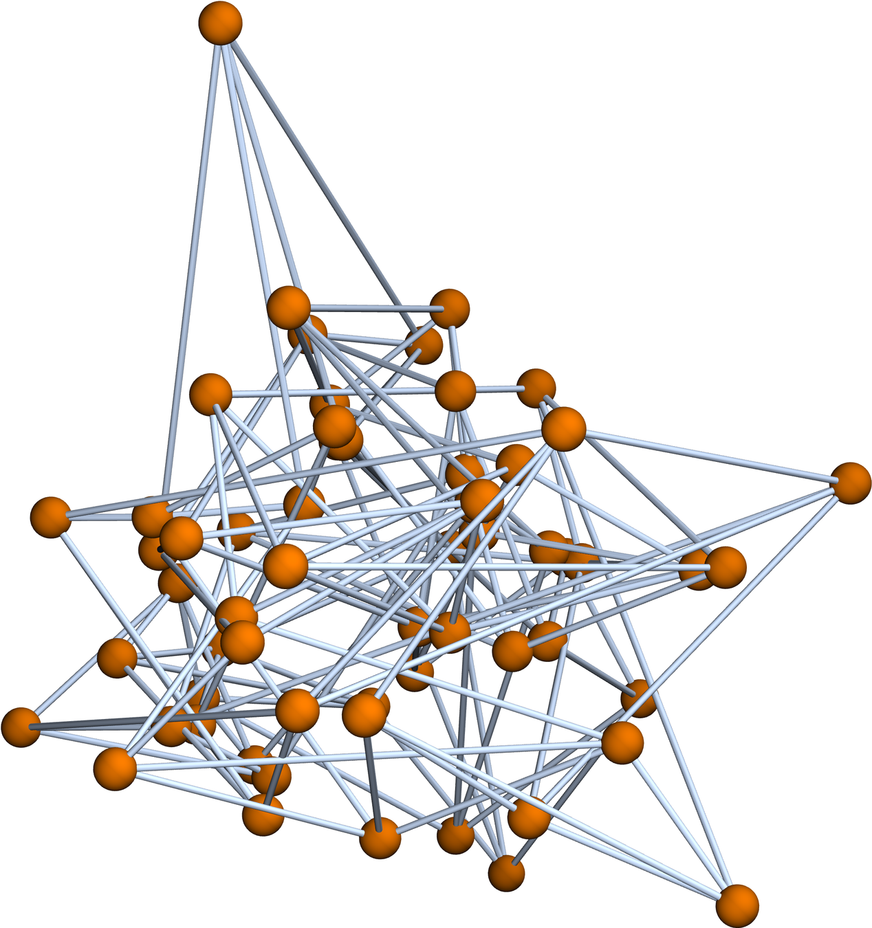
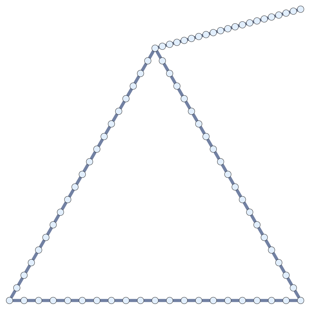
Realistic Graphs aren’t Arbitrary
Definition.
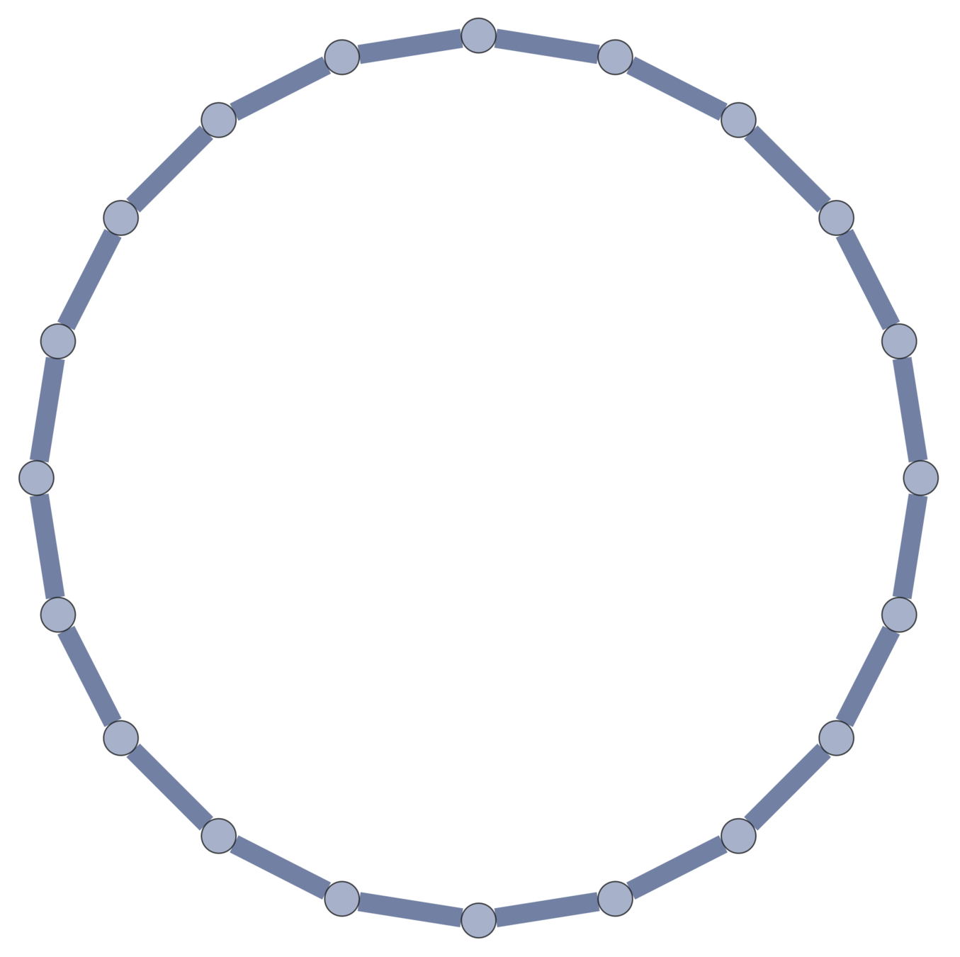
For a multigraph \(\mathcal{G}\), let \(\mathcal{G}_n\) be the graph created by subdividing each edge of \(\mathcal{G}\) into \(n\) edges.
Observation.
In synthetic polymers, \(n \sim\) # of persistence lengths along each edge of the structure graph.


Chain Maps and Structure Graphs
Idea.
The junction positions in a random embedding of a subdivided graph ought to be some random embedding of the structure graph.

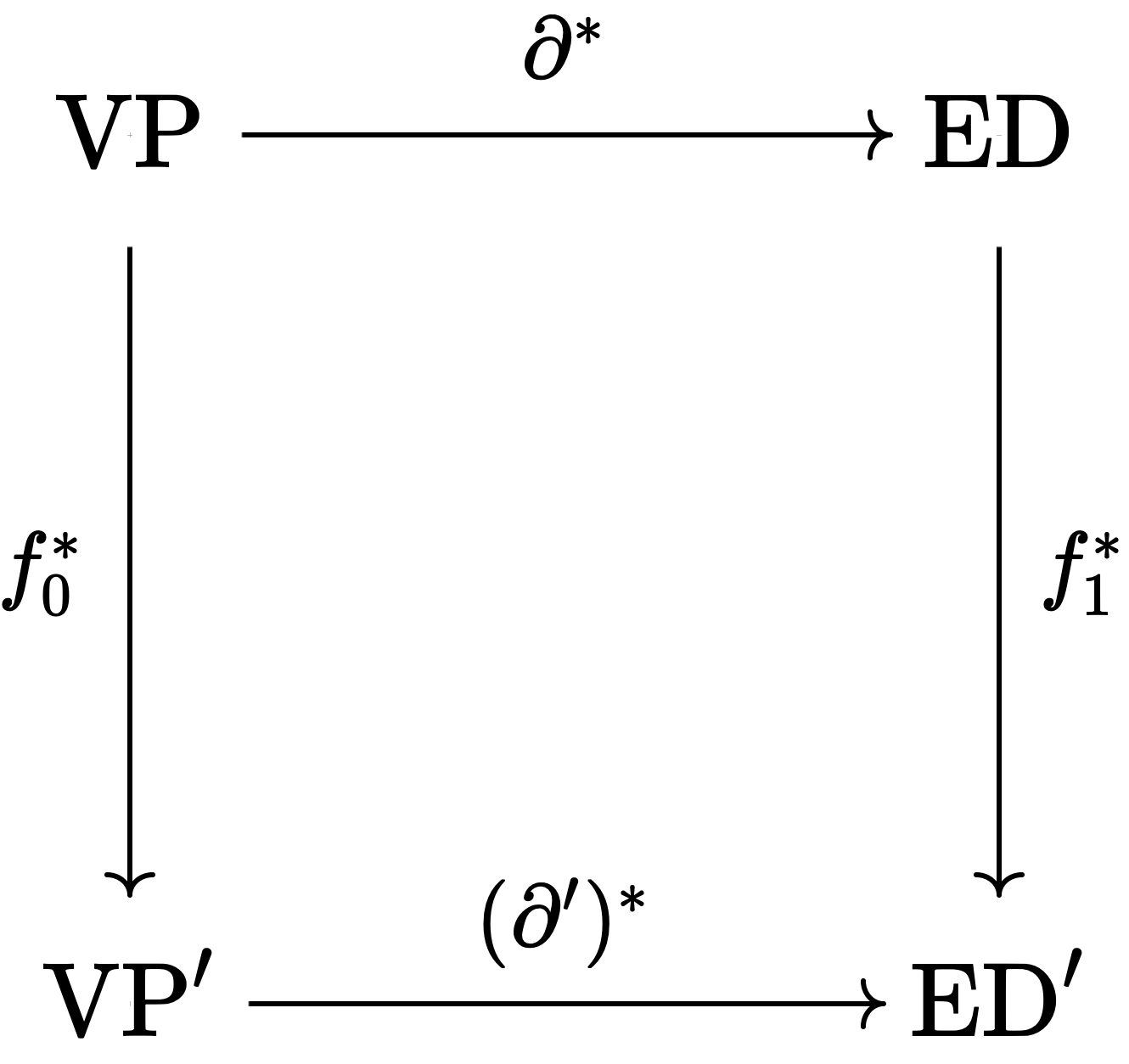
Definition.
Given \(\mathcal{G}\) and \(\mathcal{G}'\) and \(f_0: \operatorname{VC}' \to \operatorname{VC}\), \(f_1: \operatorname{EC}' \to \operatorname{EC}\), \(f_0\) and \(f_1\) are chain maps if \(\partial f_1 = f_0 \partial'\).
Structure Graph Distribution
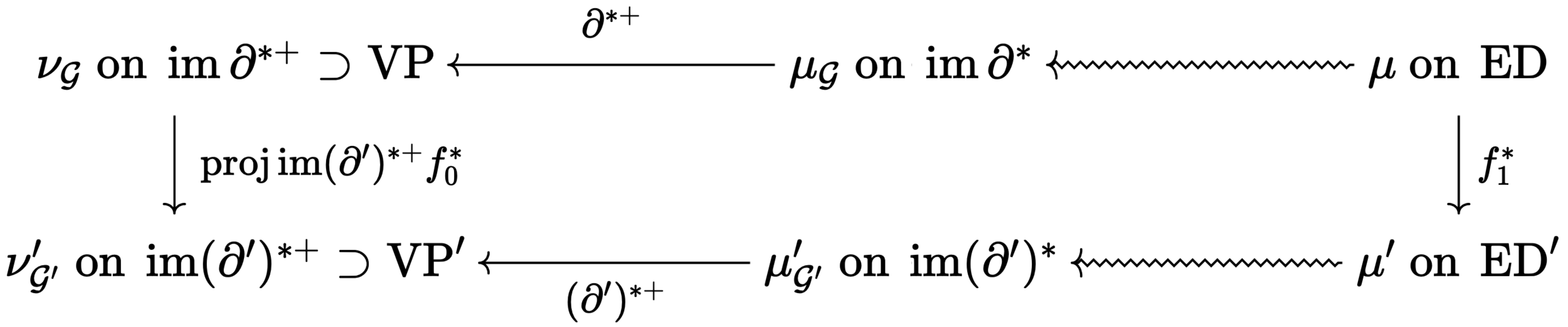
Theorem [with Cantarella, Deguchi, Uehara (2022)]
Suppose \(f_0,f_1\) are injective chain maps between \(\mathcal{G}'\) and \(\mathcal{G}\) with the same cycle rank, \(\mu\) an admissible measure on \(\operatorname{ED}\) compatible with \(\mathcal{G}\), and \(\mu' = (f_1^\ast)_\sharp\) the pushforward on \(\operatorname{ED}'\).
The probability measure \(\nu_{\mathcal{G}'}'\) on \(\operatorname{VP}'\) induced by \(\mu'\) exists and is the pushforward under \(\operatorname{proj}\operatorname{im}(\partial')^{\ast+}\) of \(\nu_{\mathcal{G}}\) on \(\operatorname{VP}\) induced by \(\mu\).
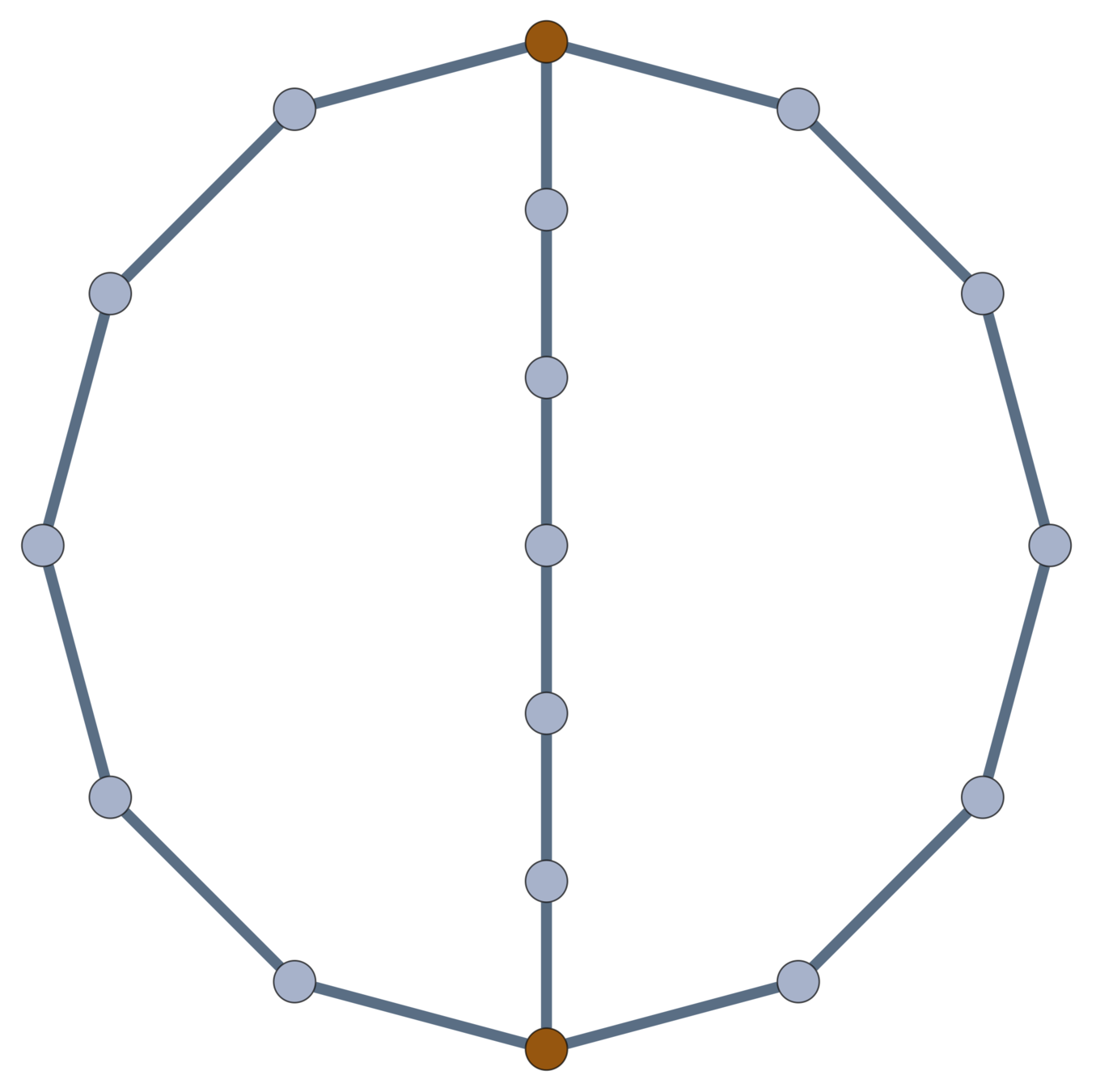
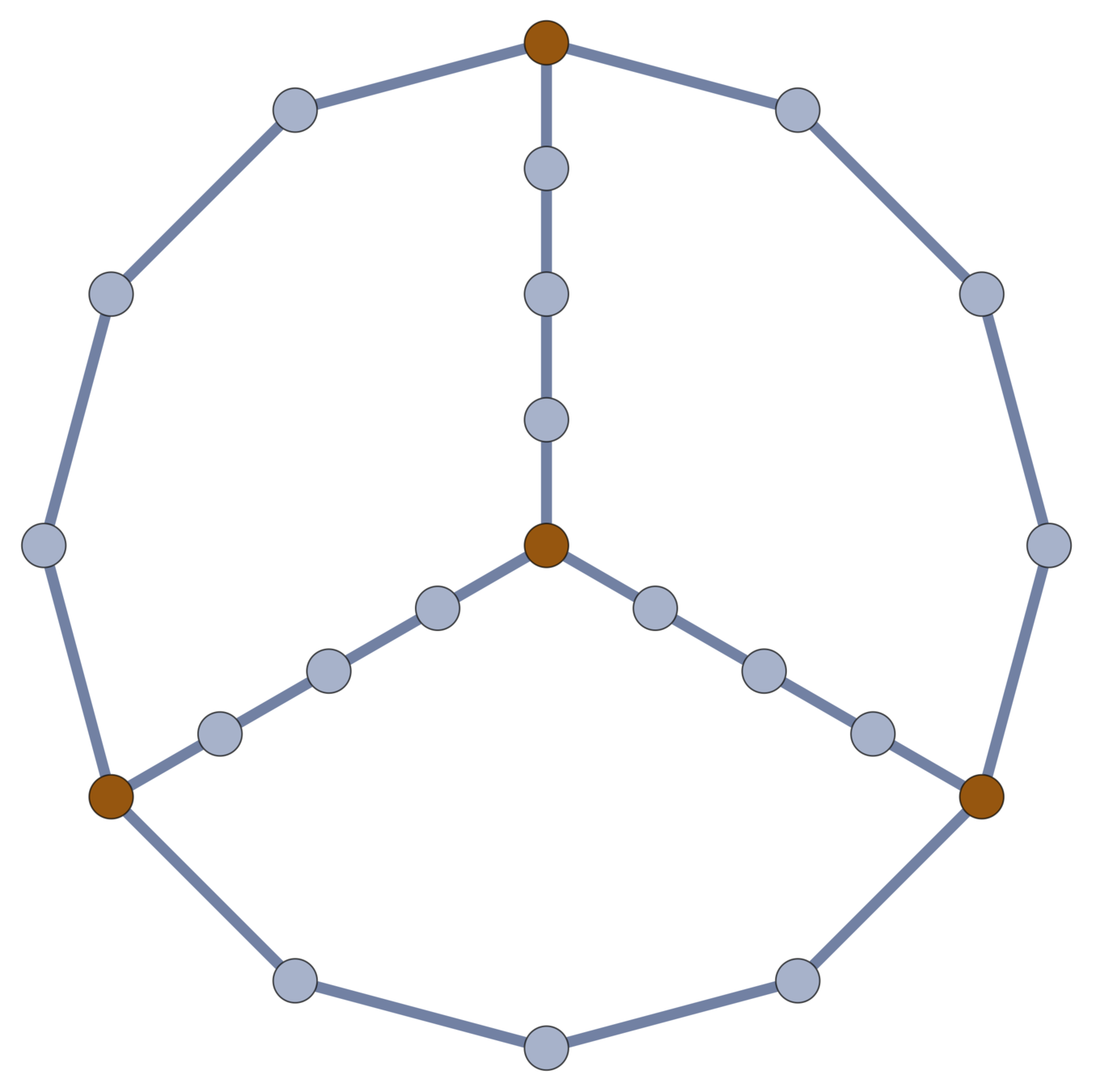
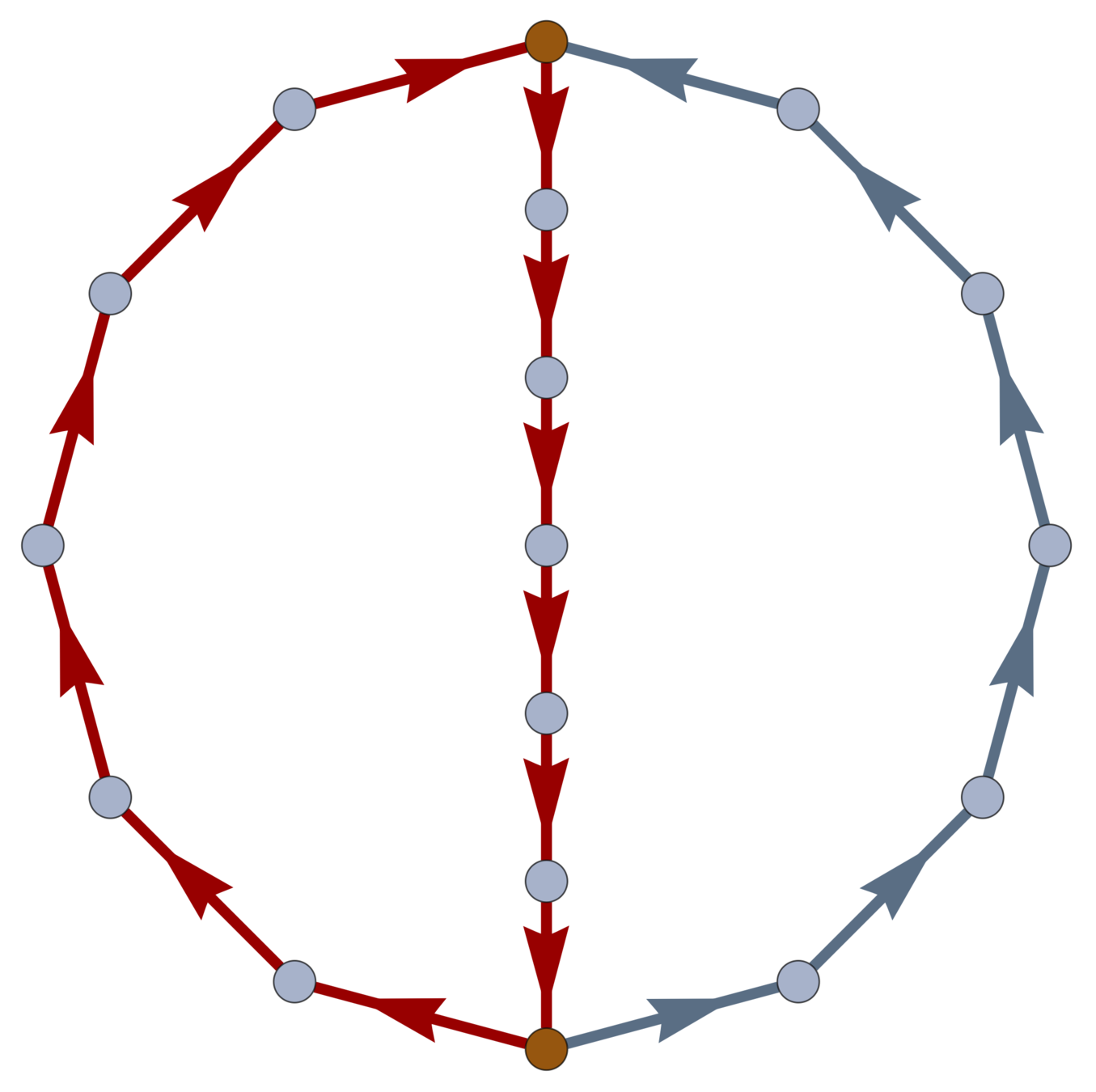
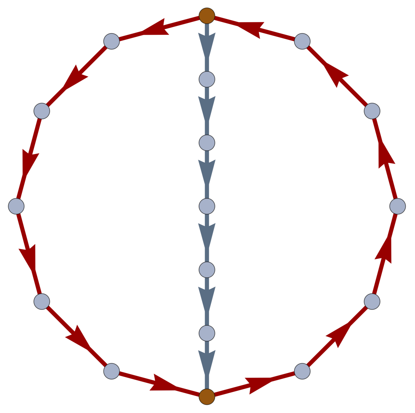
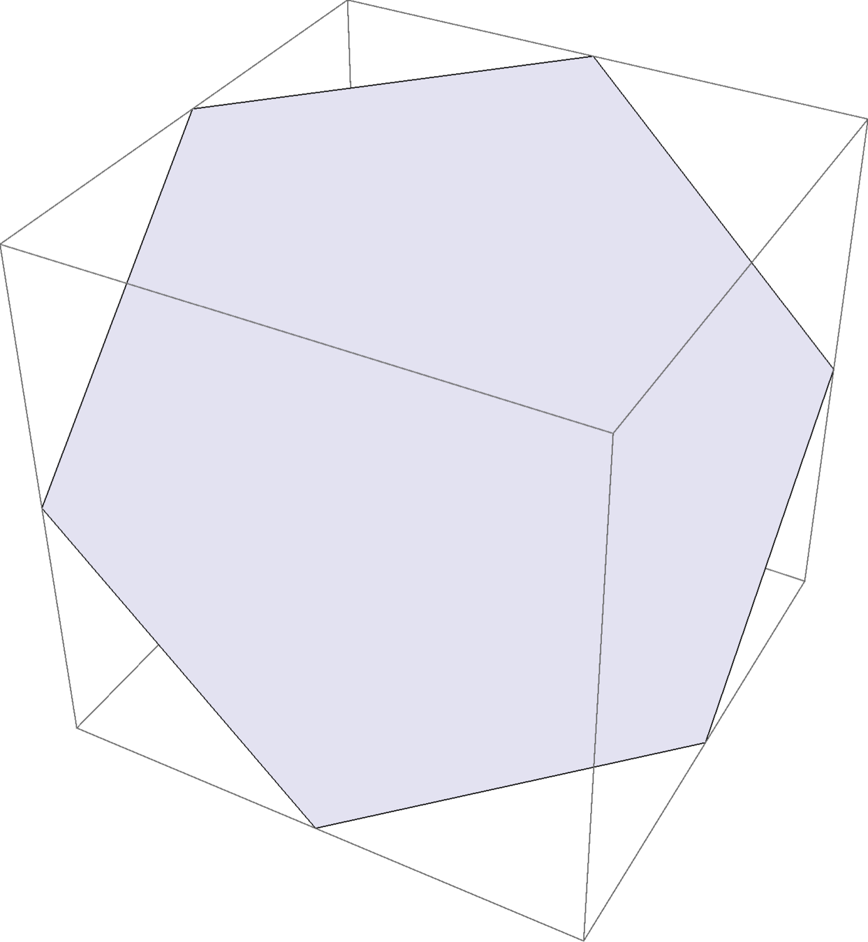
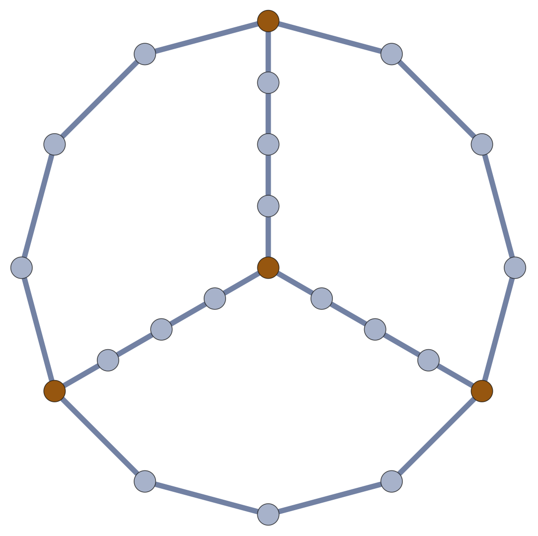
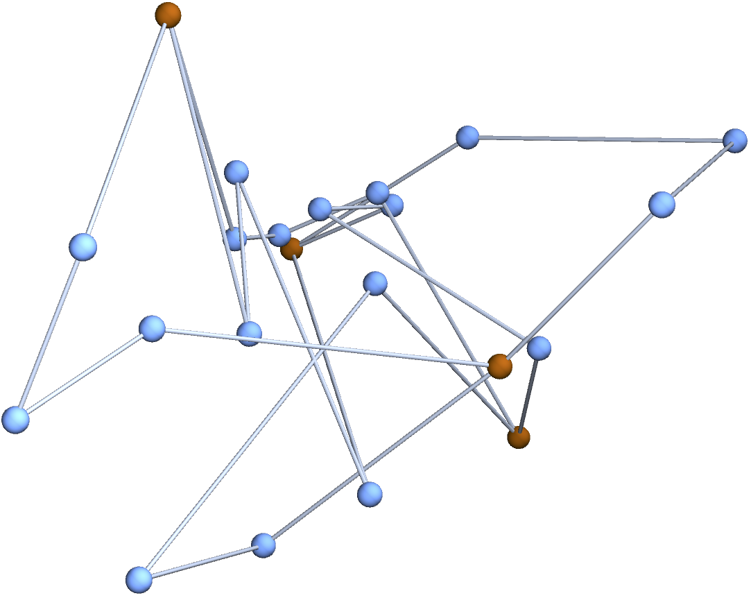
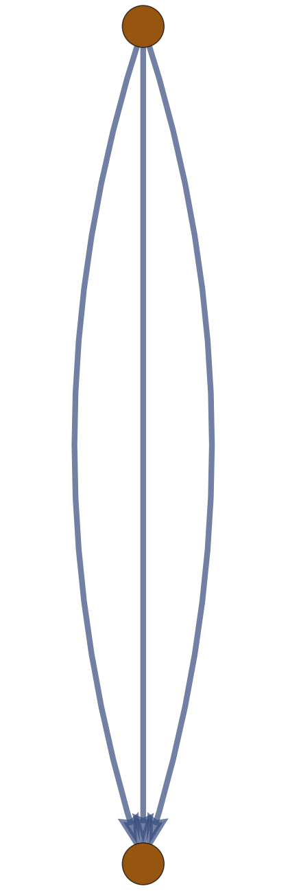
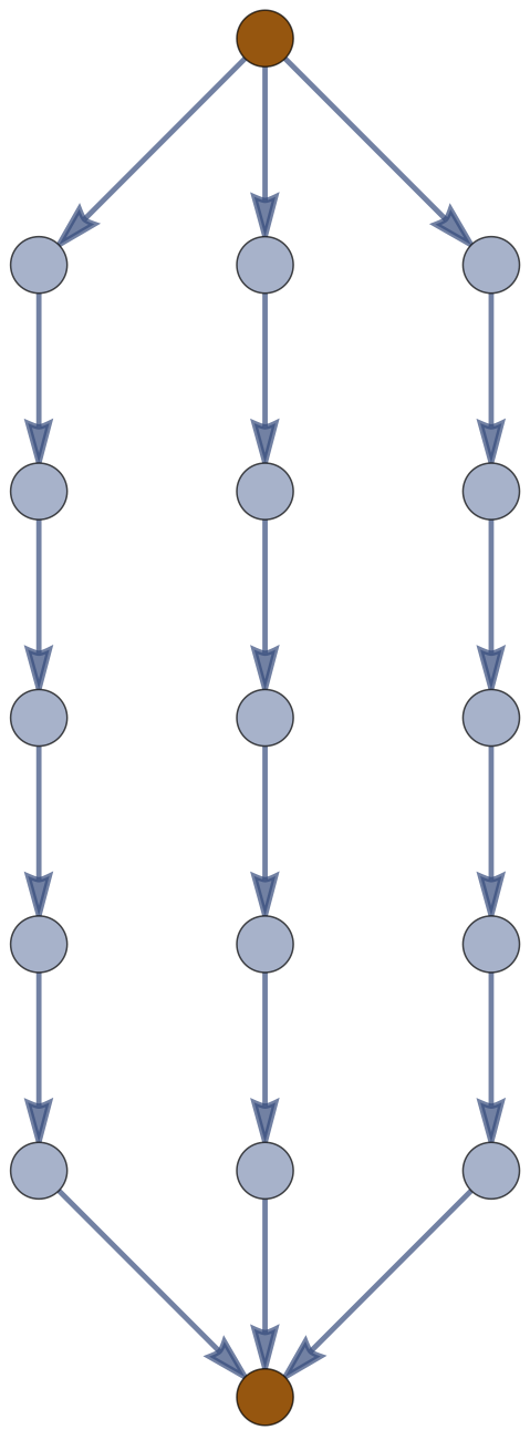
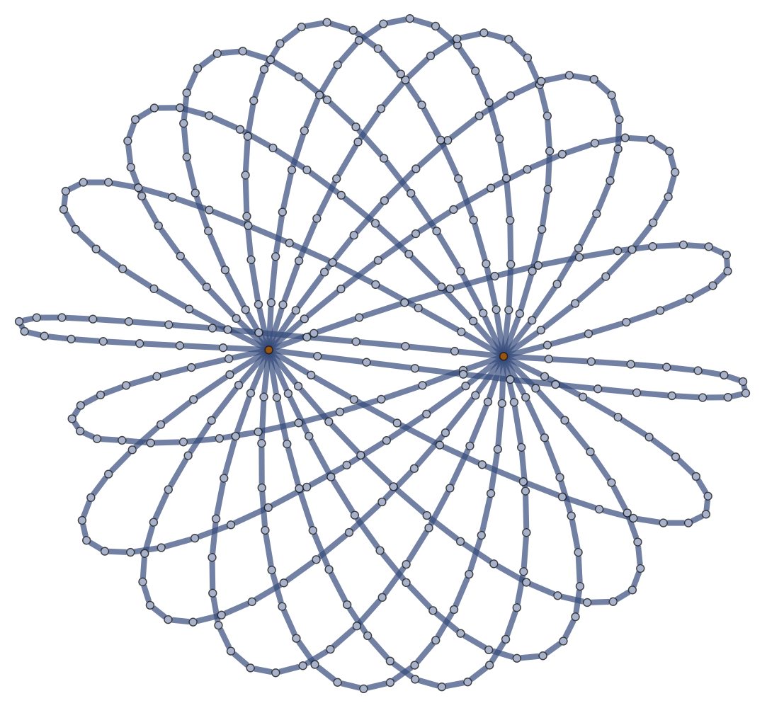
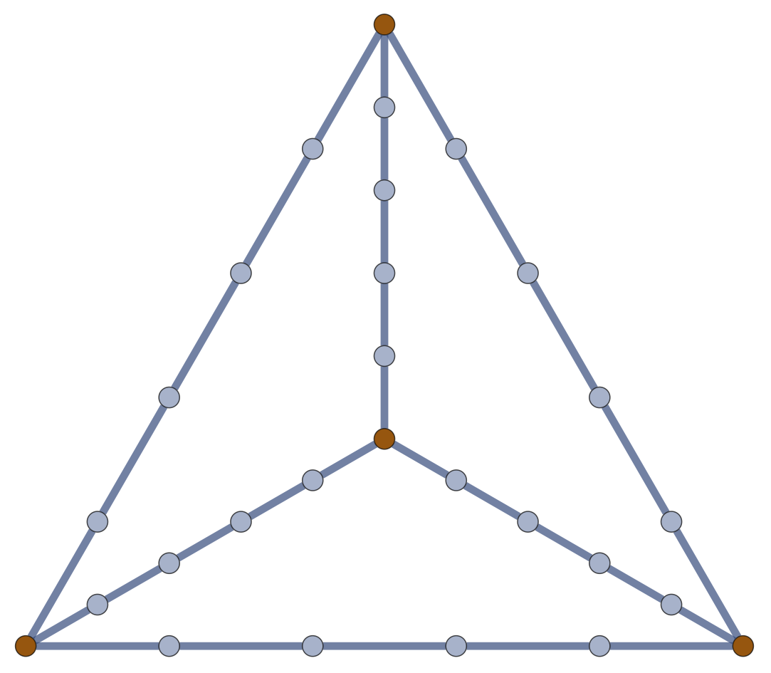
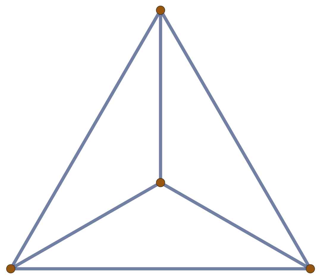
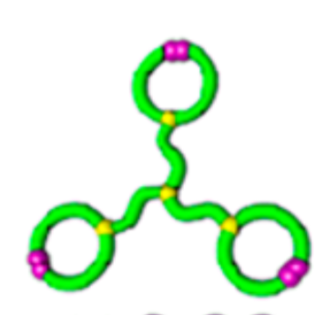
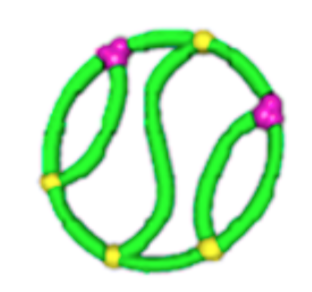
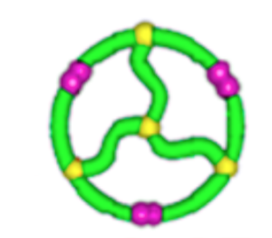
Example: \((m,n)\) \(\theta\)-Graph
Corollary.
The expected (squared) distance between junctions in an \(m\)-arc \(\theta\)-graph with \(n\) edges along each arc in a Gaussian random embedding in \(\mathbb{R}^d\) is \(d \frac{n}{m}\).
\(f_0,f_1\)
\(\mu' = \mathcal{N}(\vec{0},n)\) on \((\mathbb{R}^d)^m\)
\(\operatorname{im}(\partial')^\ast \subset \operatorname{ED}'\) is \( \operatorname{diag} \mathbb{R}^d \subset (\mathbb{R}^d)^m\)
\(\mu_{\mathcal{G}'}' = \mathcal{N}(\vec{0},n)\) on \(\operatorname{im} (\partial ')^\ast\).
\(W(w) \sim\mathcal{N}(0,\frac{n}{m})\) on coord. \(\mathbb{R}^d \subset (\mathbb{R}^d)^m\).
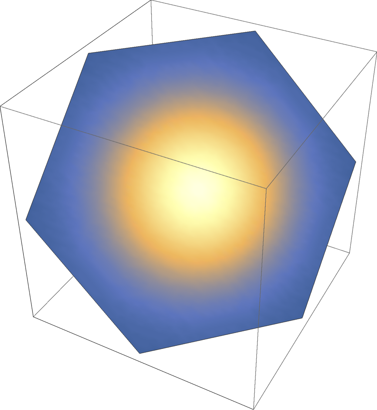
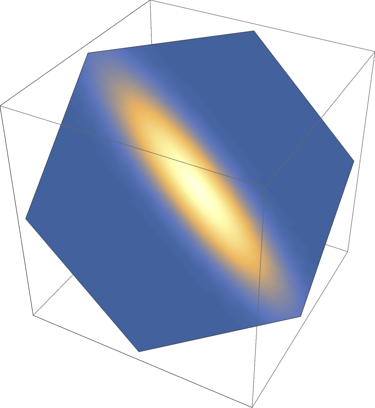
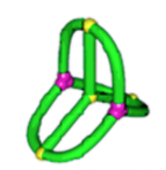
Micellation in \((m,n)\) \(\theta\)-Graph
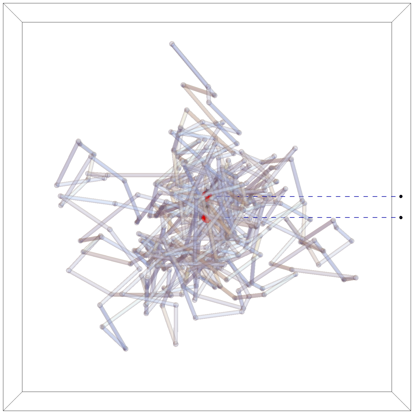
Freely-Jointed Networks
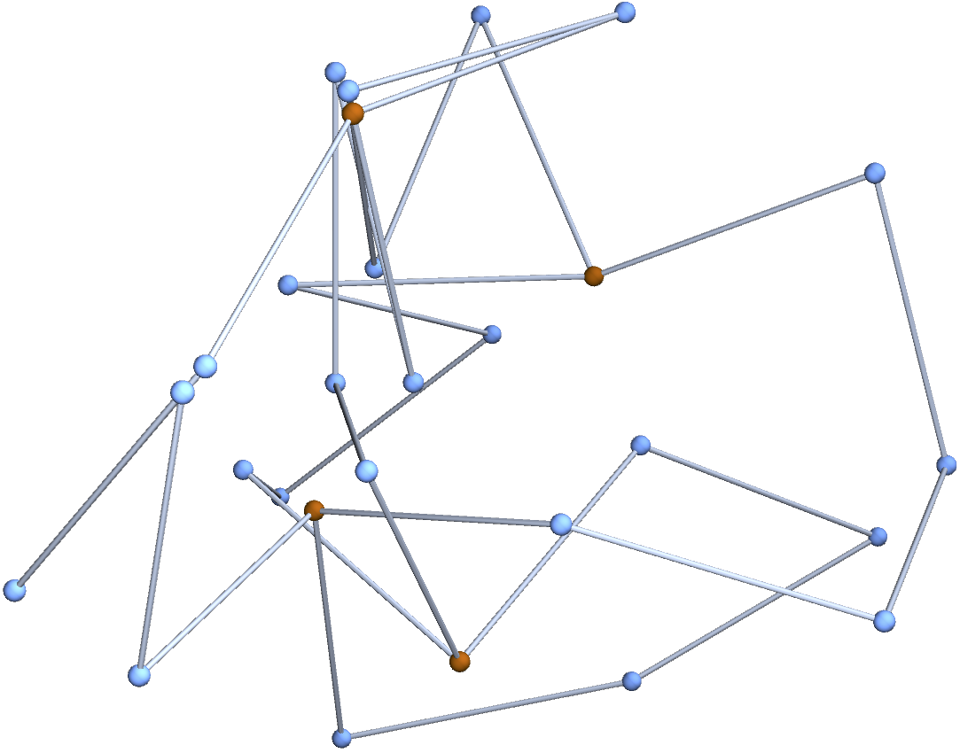
Definition.
If the measure \(\mu\) on \(\operatorname{ED}\) is the submanifold measure on the product of unit spheres \((S^2)^{\mathcal{E}} \subset \operatorname{ED} = (\mathbb{R}^3)^{\mathcal{E}}\), call the resulting model a freely jointed network.
Junction–Junction Distance
With the obvious chain maps
\(f_0,f_1\)
can compute \(\mu'\) explicitly. Junction–junction distances are explicit 6D numerical integrals.
Comparison with Markov chain experiments
What happens as \(n \to \infty\)?
Definition.
The normalized graph Laplacian \(\mathcal{L}(\mathcal{G})\) is given by
Theorem [with Cantarella, Deguchi, Uehara (2020)]
\(\lim_{n \to \infty}\frac{1}{\mathcal{V}(\mathcal{G}_n)}\mathbb{E}[R_g^2(\mathcal{G}_n)] = \frac{1}{\mathcal{E}(\mathcal{G})^2}\left(\operatorname{tr}\mathcal{L}^+(\mathcal{G})+\frac{1}{3}\operatorname{Loops}(\mathcal{G})-\frac{1}{6}\right)\).
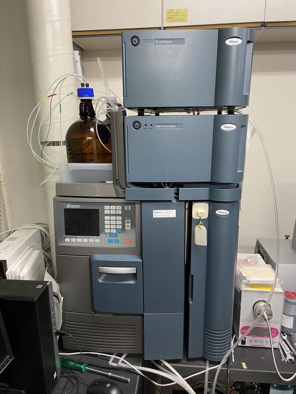
Experimental Measurements of Relative Size
Size Exclusion Chromatography apparatus
Honda Lab

relative \(\lim_{n \to \infty}\frac{1}{\mathcal{V}(\mathcal{G}_n)} \mathbb{E}[R_g^2(\mathcal{G}_n)]\)
\(\frac{17}{49}\approx 0.347\)
\(\frac{107}{245}\approx 0.437\)
\(\frac{109}{245}\approx 0.445\)
\(\frac{31}{49}\approx 0.633\)
\(\frac{43}{49}\approx 0.878\)
\(1\)
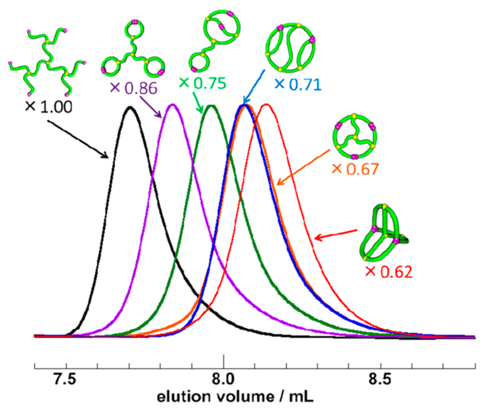
“an extremely compact 3D conformation, achieving exceptionally thermostable bioactivities”
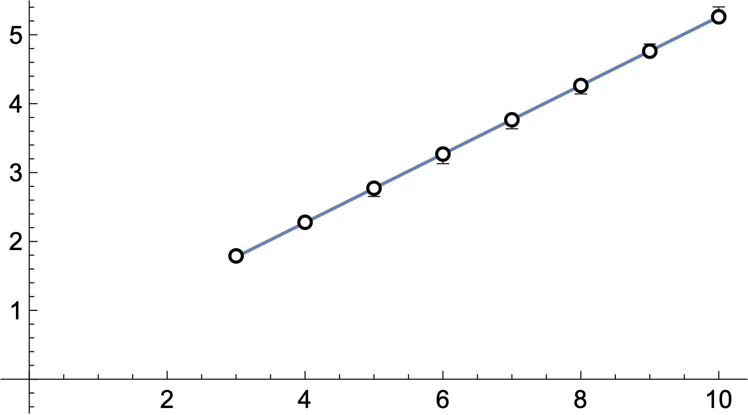
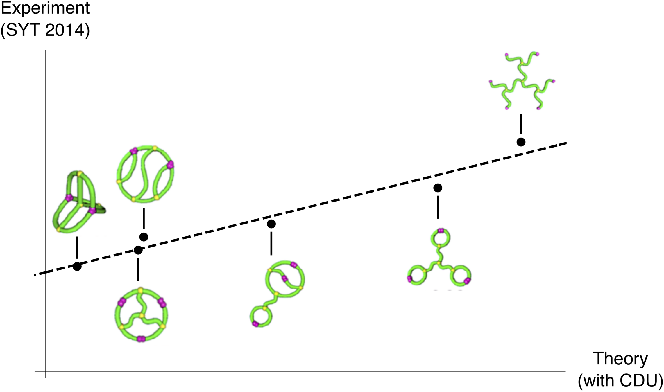
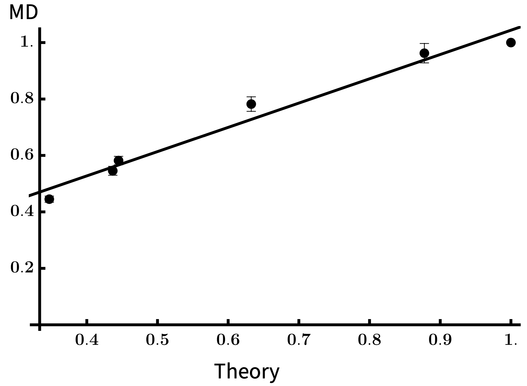
Comparing Theory and Simulation
We performed molecular dynamics simulations using LAMMPS on the TSUBAME supercomputer at Tokyo Tech. These included self-avoidance, so radii of gyration fit to
and we could estimate \(g(\mathcal{G}_\infty,\mathcal{G}_\infty^{\text{tree}}) = \frac{C_{\mathcal{G}}}{C_{\text{tree}}}\).
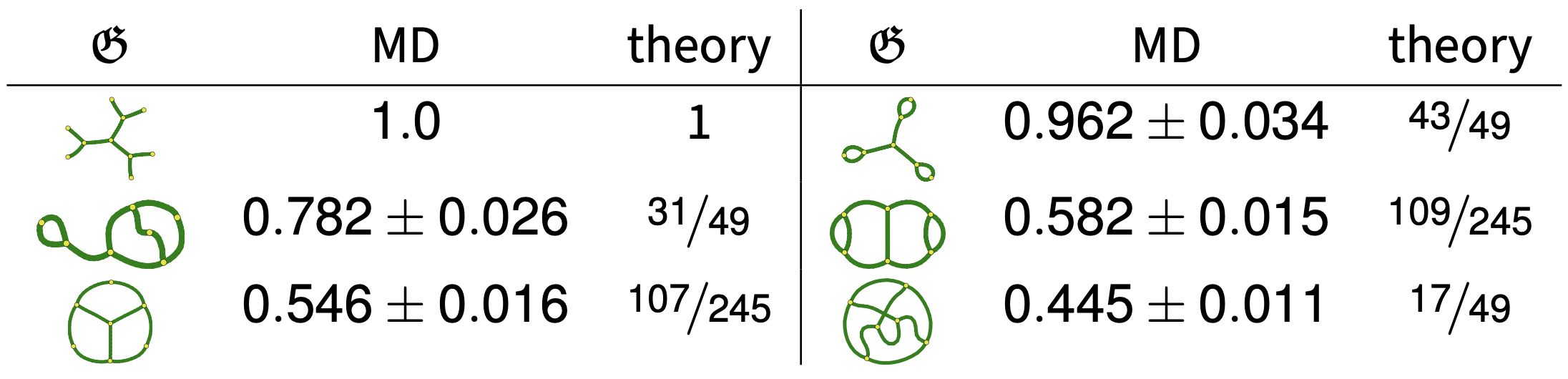
Comparing Theory and Simulation
Thank you!
References
J. Cantarella, T. Deguchi, C. Shonkwiler, E. Uehara
Radius of gyration, contraction factors, and subdivisions of topological polymers
preprint, 2020, arXiv:2004.06199
J. Cantarella, T. Deguchi, C. Shonkwiler, E. Uehara
Random graph embeddings with general edge potentials
preprint, 2022, arXiv:2205.09049