A Geometric Approach to Sampling Loop Random Flights

Clayton Shonkwiler

Colorado State University

10.19.17

Statistical physics Viewpoint

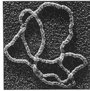
A ring polymer in solution takes on an ensemble of random shapes, with topology (knot type!) as the unique conserved quantity.

Knotted DNA

Wassermann et al.

Science 229, 171–174

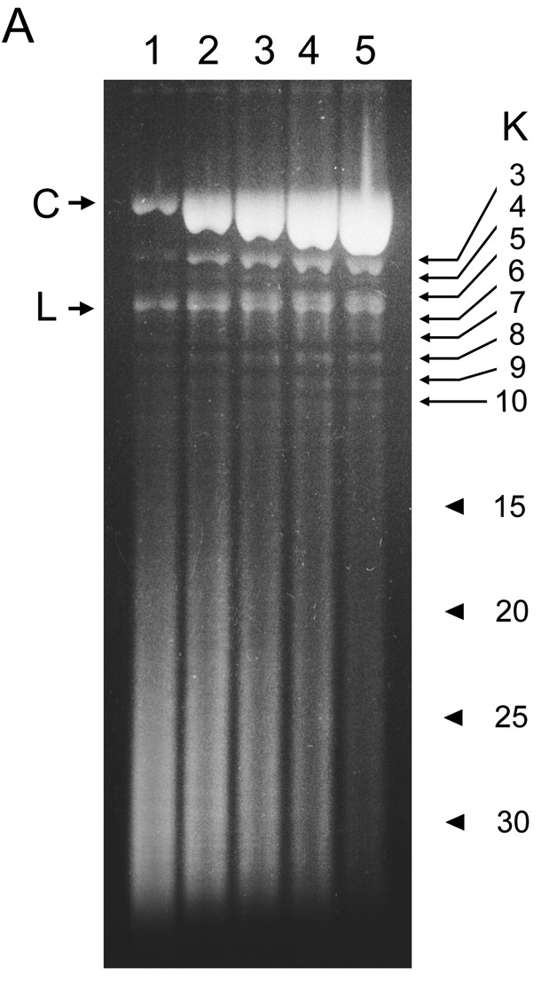
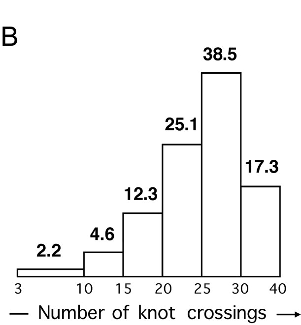
Knot complexity in DNA from P4 tailless mutants

Arsuaga et al., PNAS 99 (2002), 5373–5377

Is this surprising?

Statistical physics viewpoint

A polymer in solution takes on an ensemble of random shapes, with topology as the unique conserved quantity.

Modern polymer physics is based on the analogy between a polymer chain and a random walk.

– Alexander Grosberg

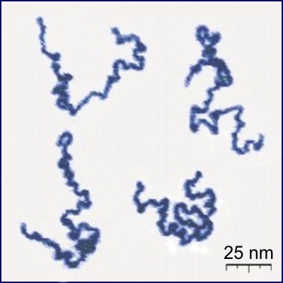
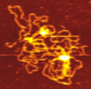
Protonated P2VP

Roiter/Minko

Clarkson University

Plasmid DNA

Alonso–Sarduy, Dietler Lab

EPF Lausanne

Sampling random flights is easy

Generate \(n\) independent uniform random points on \(S^2\) and treat them as an ordered list of edge vectors.

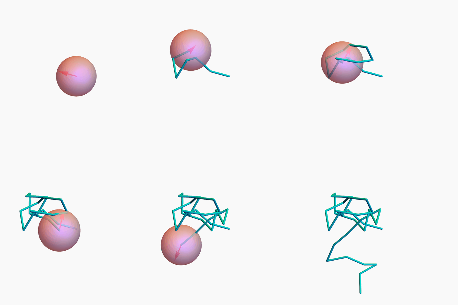
...but sampling random polygons is hard

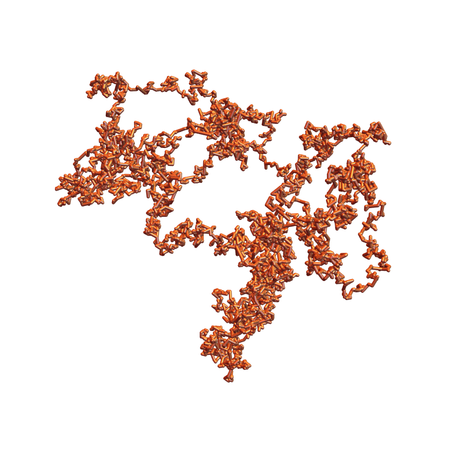
Alvarado, Calvo, Millett, J. Stat. Phys. 143 (2011), 102–138

Ansatz

Random Polygon \(\Leftrightarrow\) point in some (nice!) conformation space

Knowledge of the (differential, symplectic, algebraic) geometry of these conformation spaces leads to both

theorems and fast numerical algorithms for studying and comparing polygons in \(\mathbb{R}^3\).

The measure

The edges of an \(n\)-gon (up to translation) are unit vectors, so the space of \(n\)-gons is the submanifold of \((S^2)^n\) implicitly defined by \(e_1 + \ldots + e_n = 0\), which is codimension 3.

The natural measure is Hausdorff measure; equivalently, the volume form induced by the Riemannian submanifold metric.

A random closed \(n\)-edge polygon is a \(k\)-edge random flight and an \((n-k)\)-edge random flight, conditioned on having the same end-to-end distance.

Key Idea

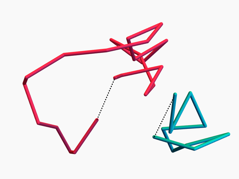
Density of the end-to-end distance

Classical Fact: The density of the end-to-end vector of an \(n\)-step random walk is

\phi_n(\ell) = \frac{2\ell}{\pi} \int_0^\infty x \sin \ell x \,\mathrm{sinc}^n x \,\mathrm{d}x

= \frac{2^{-n-1}}{\pi \ell(n-2)!} \sum_{k=0}^{n-1} (-1)^k \binom{n-1}{k} \left([-2k+\ell +n-2]_+^ {n-2}\right.

\left.- [-2 k+\ell +n]_+^{n-2}\right)

Proof: Fourier transform (since \(\mathrm{sinc}\) is the transform of the boxcar function).

This is piecewise-polynomial in \(\ell\) of degree \(n-3\)

Density of a polygon chord

Proposition (with Cantarella) The pdf of the chord connecting \(v_1\) with \(v_{k+1}\) in an \(n\)-gon is

\frac{4 \pi \ell^2}{C_n} \phi_k(\ell) \phi_{n-k}(\ell)

where \(C_n = 2^{n-5}\pi^{n-4} \int_{-\infty}^{\infty} x^2 \,\mathrm{sinc}^n x \,\mathrm{d}x\).

Fact: This is piecewise-polynomial in \(\ell\) of degree \(n-4\).

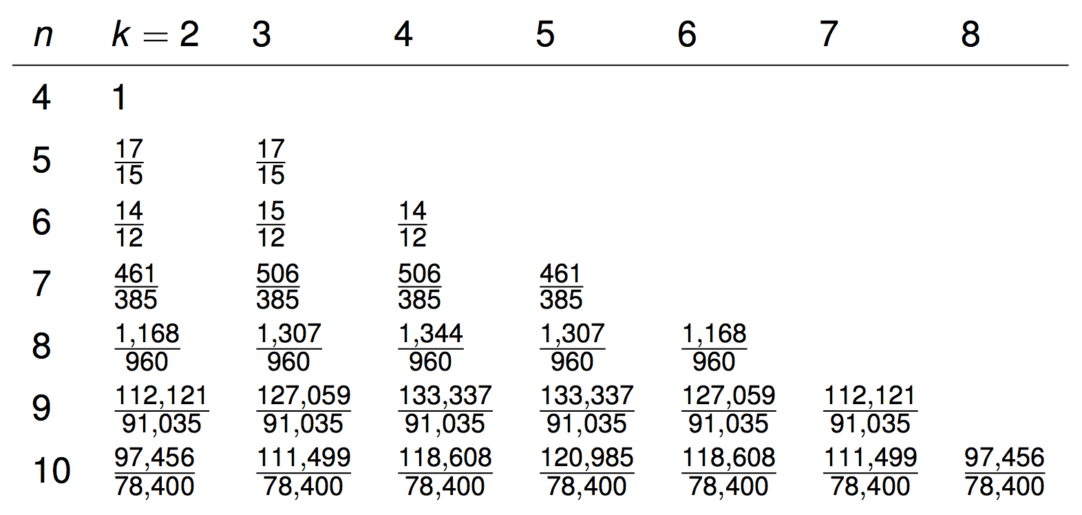
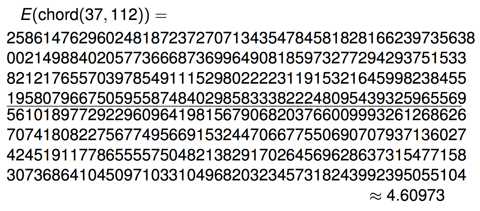
Expected values of chordlengths

Questions

Why are the expectations rational?

Why degree \(n-4\)?

Where are these crazy polynomials coming from?

Continuous symmetry \(\Rightarrow\) conserved quantity

Some classical mechanics

Duistermaat–Heckman Theorem (stated informally)

On a \(2m\)-dimensional symplectic manifold, \(d\) commuting Hamiltonian symmetries (a Hamiltonian \(T^d=(S^1)^d\)-action) induce \(d\) conserved quantities (momenta).

The joint distribution of the momenta on \(\mathbb{R}^d\) is continuous, piecewise polynomial, degree \(\leq m-d\).

Symplectic what?

A symplectic manifold \((M,\omega)\) is an even-dimensional manifold \(M\) together with a closed, non-degenerate 2-form \(\omega\).

Example: \((S^2,d\theta\wedge dz)\)

Example: \((\mathbb{R}^2,dx \wedge dy) = (\mathbb{C},\frac{i}{2}dz \wedge d\bar{z})\)

Example: \((T^*\mathbb{R}^n, \sum_{i=1}^n dq_i \wedge dp_i)\)

Example: \((S^2,\omega)\), where \(\omega_p(u,v) = (u \times v) \cdot p\)

Example: \((\mathbb{R}^2,\omega)\) where \(\omega(u,v) = \langle i u, v \rangle \)

This is the right setting for Hamiltonian mechanics.

Example: \((\mathbb{C}^n, \frac{i}{2} \sum dz_k \wedge d\overline{z}_k)\)

Duistermaat what?

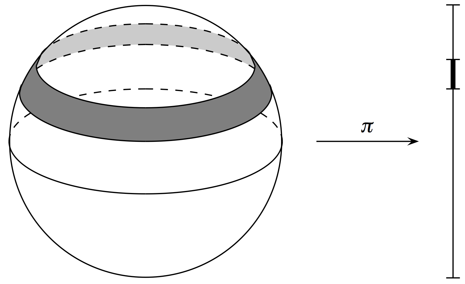
Theorem (Archimedes, Duistermaat–Heckman)

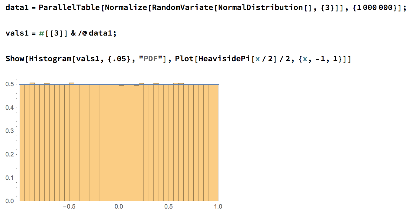
Let \(f: S^2 \to \mathbb{R}\) be given by \(f(x,y,z) = z\). Pushing forward the uniform measure on \(S^2\) to the image \([-1,1]\) gives Lebesgue measure.

A higher-dimensional example

Proposition If we rotate both factors of \(S^2 \times S^2\) simultaneously around the \(z\)-axis, the conserved quantity is \(z_1 + z_2\), and the pushforward measure on \([-2,2]\) has density given by the triangle function.

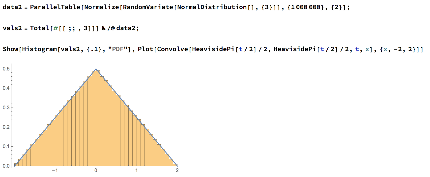
Why degree \(n-4\)?

Duistermaat–Heckman Theorem (stated informally) On a \(2m\)-dimensional symplectic manifold, \(d\) commuting Hamiltonian symmetries (a Hamiltonian \(T^d\)-action) induce \(d\) conserved quantities (momenta).

The joint distribution of the momenta is continuous, piecewise polynomial, degree \(\leq m-d\).

\(n\)-gons up to rotation are \(2m=(2n-6)\)-dimensional, so chord length is piecewise polynomial of degree \(\leq\)

\(m-1=(n-3)-1=n-4\)

We actually have more symmetries!

\(n-3\) commuting symmetries

Rotations around \(n-3\) chords \(d_i\) by \(n-3\) angles \(\theta_i\) commute.

Main Theorem

Theorem (with Cantarella, ’16)

The joint distribution of \(d_1,\ldots , d_{n-3}\) and \(\theta_1, \ldots , \theta_{n-3}\) are all uniform on their domains.

Proof: Check that D–H applies (this is the hard part, since the torus action is not defined everywhere).

Then count: \(m=n-3\) and we have \(d=n-3\) symmetries, so the pdf of the \(d_i\) is piecewise polynomial of degree \(\leq\)

\(m-d = (n-3)-(n-3)=0\).

Since the pdf is continuous and the domain is connected, it must be constant.

Definition: If \((M,\omega)\) is \(2m\)-dimensional and has \(m\) commuting symmetries, we call \(M\) toric.

A polytope

The \((n-3)\)-dimensional moment polytope \(\mathcal{P}_n \subset \mathbb{R}^{n-3}\) is defined by the triangle inequalities

0 \leq d_i \leq 2

1 \leq d_i + d_{i-1}

|d_i - d_{i-1}| \leq 1

0 \leq d_{n-3} \leq 2

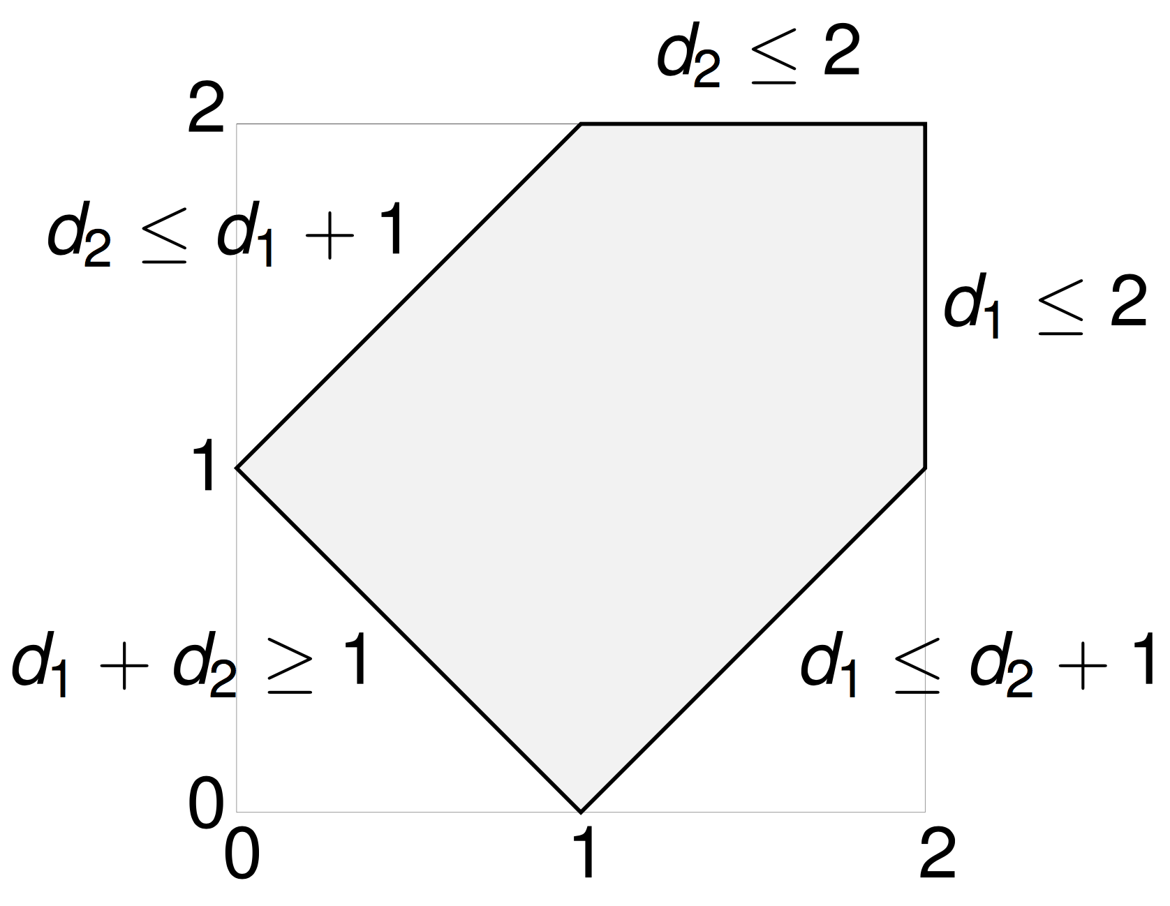
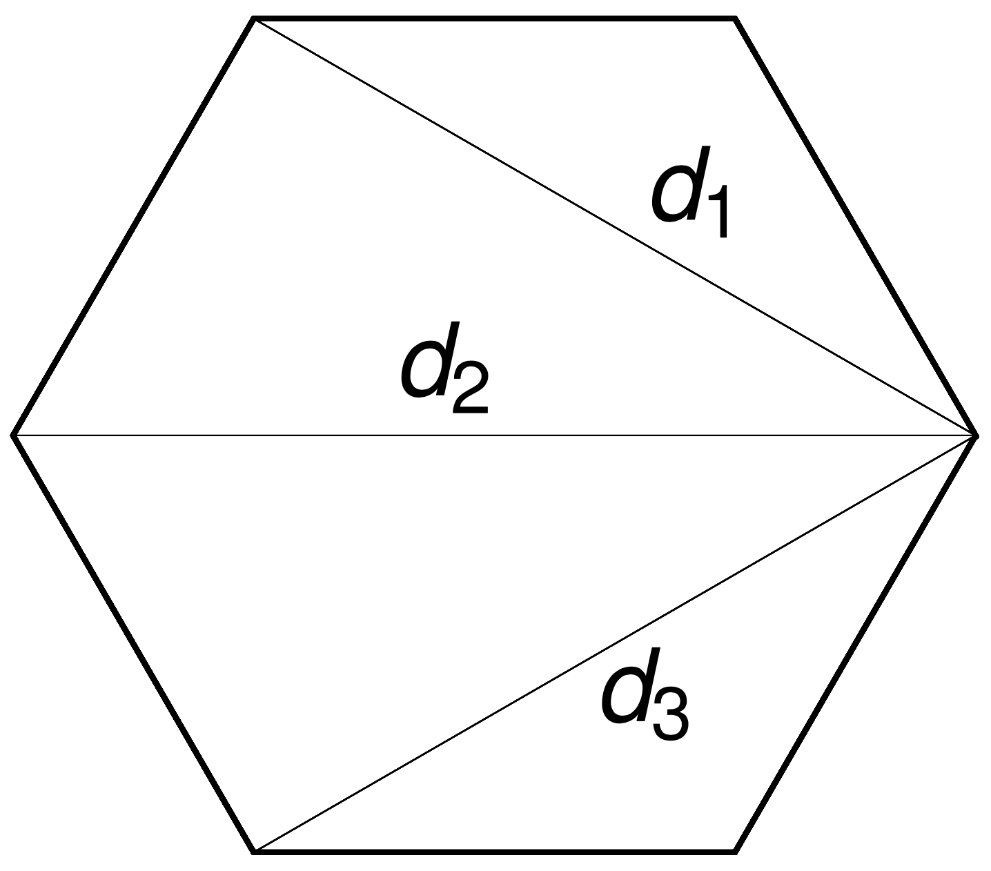
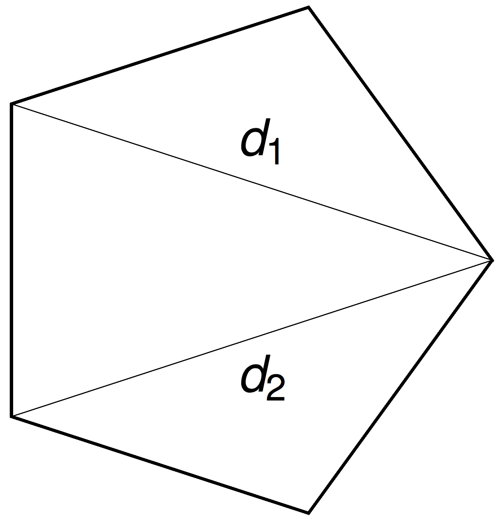
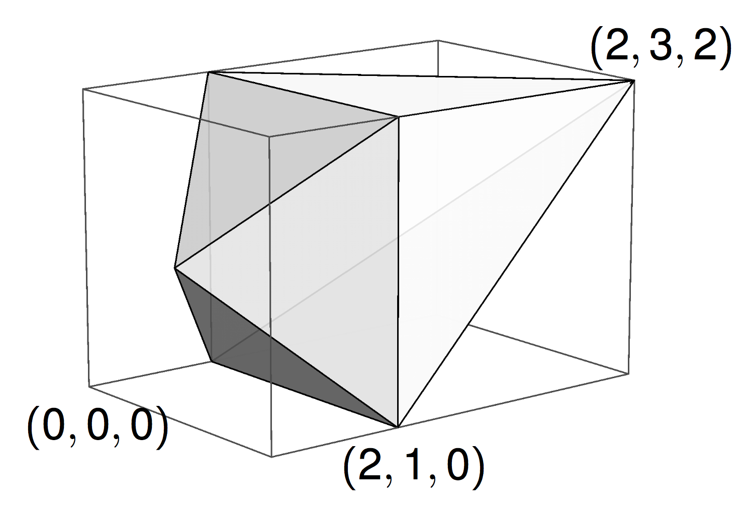
From action-angle coordinates to polygons

There exists an almost-everywhere defined map \(\alpha: \mathcal{P}_n \times (S^1)^{n-3} \to \{n\text{-gons}\}\) which is measure-preserving.

This is only sensible as a map to polygons modulo translation and rotation.

Sampling

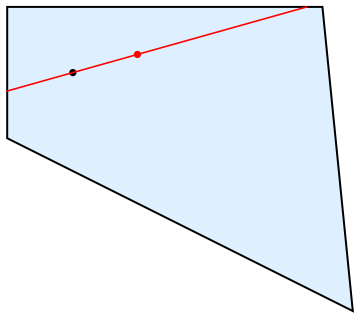
We have reduced the problem of sampling a random polygon to the problem of sampling a (specific) convex polytope.

Theorem (Smith, 1984)

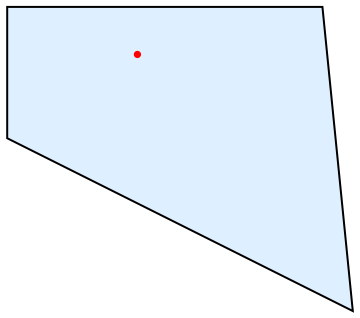
For any convex polytope \(\mathcal{P}\), the hit-and-run Markov chain is uniformly ergodic with respect to Lebesgue measure on \(\mathcal{P}\).

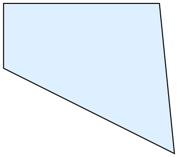
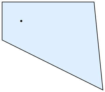
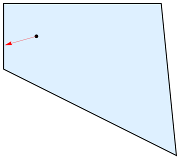
Toric Symplectic Markov Chain Monte Carlo

Definition (TSMCMC\((\beta)\))

If \(x_k = (p_k,\theta_k) \in \mathcal{P_n} \times T^{n-3}\), define \(x_{k+1}\) by:

With probability \(\beta\), update \(p_k\) by a hit-and-run step on \(\mathcal{P}_n\)
Else, replace \(\theta_k\) by a new point sampled uniformly from \(T^{n-3}\)

At each step, construct the corresponding polygon \(\alpha(p_n, \theta_n)\).

Theorem (with Cantarella, 2016)

TSMCMC(\(\beta\)) is uniformly ergodic with respect to the standard probability measure on random polygons modulo translation and rotation.

More generally...

Theorem (with Cantarella, 2016)

If \((M,\omega)\) is toric symplectic with moment polytope \(\mathcal{P} \subset \mathbb{R}^m\), then TSMCMC(\(\beta\)) on \(\mathcal{P} \times T^m\) is uniformly ergodic with respect to the symplectic volume measure on \(M\).

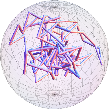
For example, polygons in (rooted) spherical confinement.

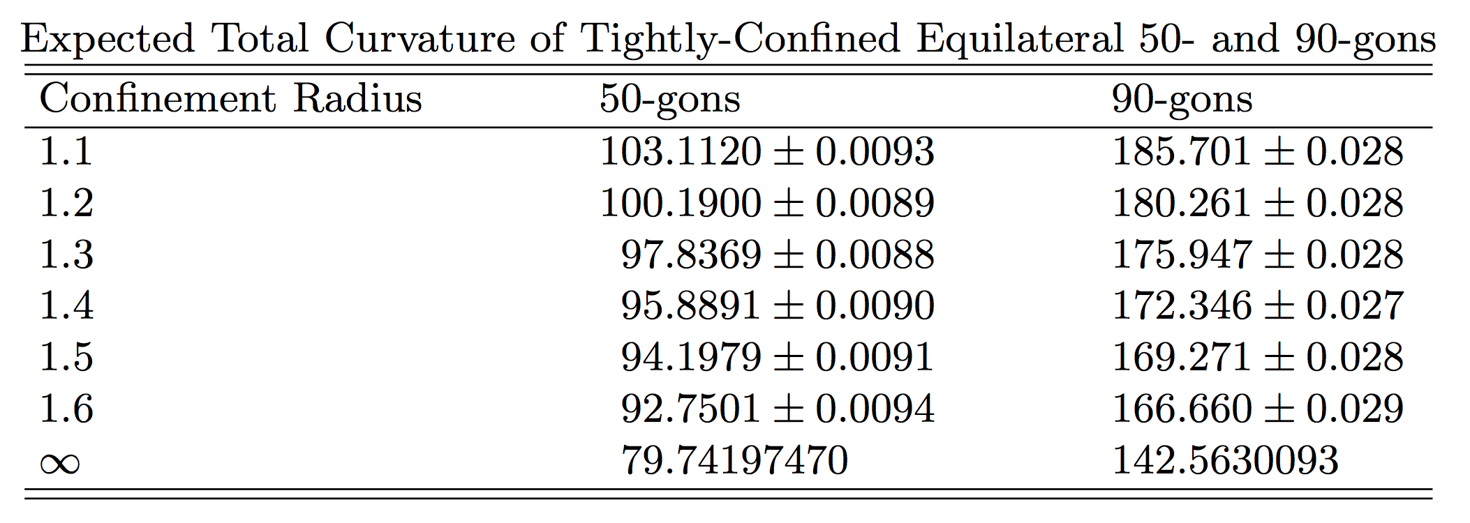
Expected Total Curvature

Direct Sampling

For unconfined polygons, we can do better: no Markov chains required!

Introduce fake chordlengths \(d_0=1=d_{n-2}\) and make the linear change of variables

\(s_i = d_i - d_{i-1} \text{ for } 1 \leq i \leq n-2\).

Then \(\sum s_i = d_{n-2} - d_0 = 0\), so \(s_{n-2}\) is determined by \(s_1, \ldots , s_{n-3}\)

and the inequalities

0 \leq d_i \leq 2

1 \leq d_i + d_{i-1}

|d_i - d_{i-1}| \leq 1

0 \leq d_{n-3} \leq 2

become

\(-1 \leq s_i \leq 1, -1 \leq \sum_{i=1}^{n-3} s_i \leq 1\)

\(\sum_{j=1}^i s_j + \sum_{j=1}^{i+1}s_j \geq -1\)

The polytope is surprisingly large!

Let \(\mathcal{C}_n \subset \mathbb{R}^{n-3}\) be determined by

\(-1 \leq s_i \leq 1, -1 \leq \sum_{i=1}^{n-3} s_i \leq 1\)

\(\sum_{j=1}^i s_j + \sum_{j=1}^{i+1}s_j \geq -1\)

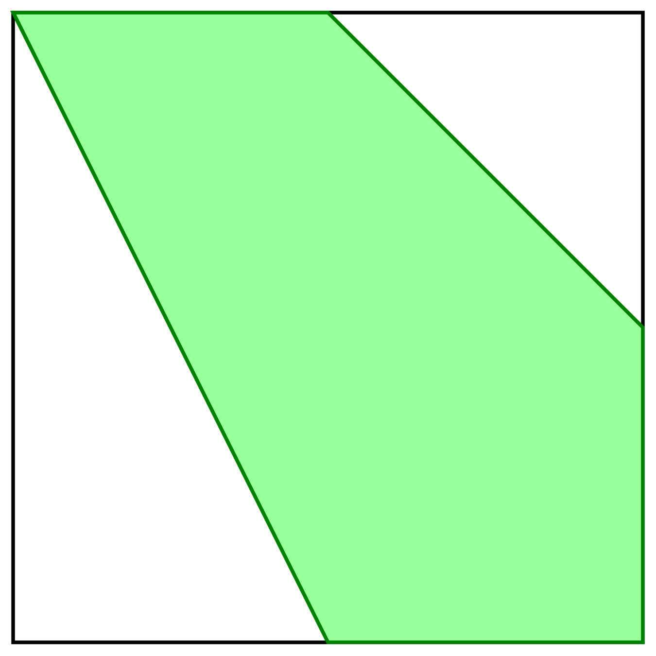
\(\mathcal{C}_5\)

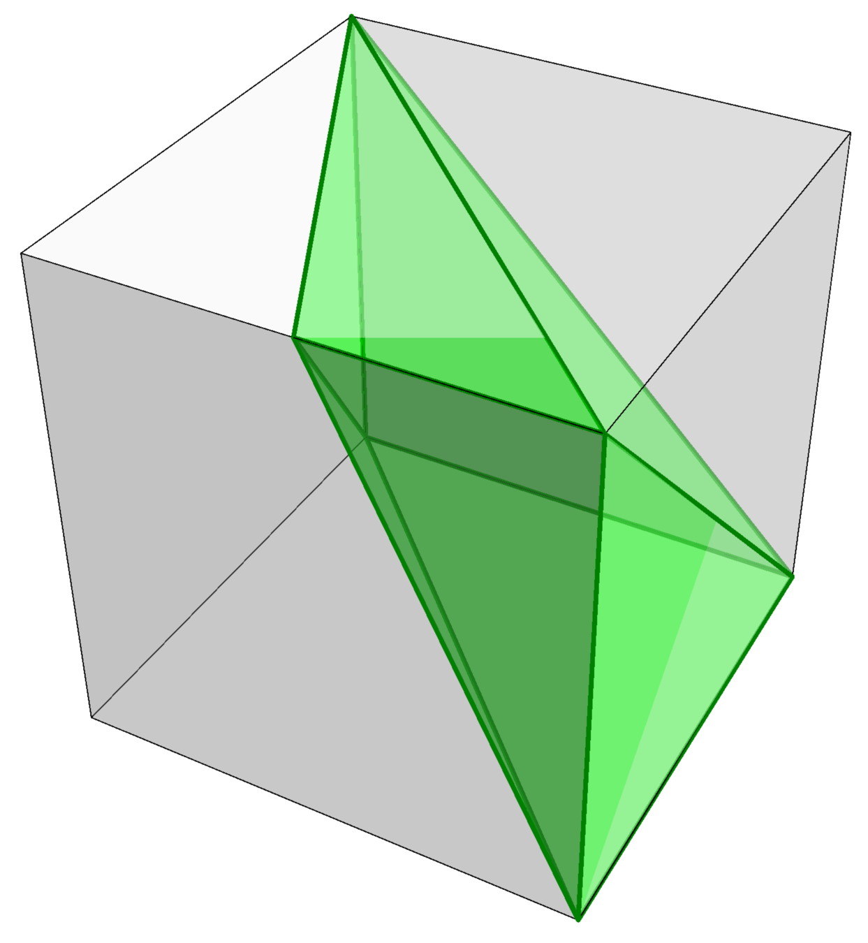
\(\mathcal{C}_6\)

Proposition (with Cantarella, Duplantier, Uehara, 2016)

The probability that a point in the hypercube lies in \(\mathcal{C}_n\) is asymptotic to

\(6 \sqrt{\frac{6}{\pi}}\frac{1}{n^{3/2}}\)

The volume of \(\mathcal{C}_n\)

Theorem (Khoi, Takakura, Mandini, 2000s)

The volume of \(\mathcal{C}_n\) is exactly

\text{Vol} (\mathcal{C}_n) = \frac{1}{2 (n-3)!}\sum_{k=0}^{\left\lfloor \frac{n}{2}\right\rfloor} (-1)^{k+1} \binom{n}{k}(n-2 k)^{n-3}

Observation (Edwards, 1922)

\text{Vol}(\mathcal{C}_n) = \frac{2^{n-1}}{2\pi} \int_{-\infty}^\infty \frac{\sin^n x}{x^{n-2}}dx

[T]here is in these days far too great a tendency on the part of teachers to push on their pupils so fast to the Higher Branches of Analysis or to Physical Mathematics that many have neither time nor opportunity for the cultivation of real personal proficiency, or for the acquirement of that individual manipulative skill which is essential to any real confidence of the student in his own power to conduct unaided investigation.

= \frac{2^{n-1}}{2\pi} \int_{-\infty}^\infty \mathrm{sinc}^n( x) x^2 dx

= \frac{2^{n-1}}{2\pi}\int_{-\infty}^\infty \mathrm{sinc}^n\left(\frac{y}{\sqrt{n}}\right) \frac{y^{2}dy}{n^{3/2}}

x=\frac{y}{\sqrt{n}}

\mathrm{sinc}\left(\frac{y}{\sqrt{n}}\right)=1-\frac{y^2}{6n}+o\left(\frac{1}{n}\right)

\lim_{n \to \infty} \left(1-\frac{a}{n}+o\left(\frac{1}{n}\right)\right)^n=e^{-a}

\sim \frac{2^{n-1}}{2\pi}\frac{1}{n^{3/2}} \int_{-\infty}^\infty e^{-\frac{y^2}{6}} y^{2} dy

= 3 \, \sqrt{\frac{3}{\pi }} \, 2^{n-\frac{3}{2}} \, \frac{1}{n^{3/2}}

Direct sampling

Action-Angle Method

Theorem (with Cantarella, Duplantier, Uehara, 2016)

The action-angle method directly samples polygon space in expected time \(\Theta(n^{5/2})\).

Generate \((s_1,\ldots , s_{n-3})\) uniformly on \([-1,1]^{n-3}\)
Test whether \((s_1,\ldots , s_{n-3})\in \mathcal{C}_n\)
Change to \((d_1, \ldots , d_{n-3})\) coordinates
Generate dihedral angles from \(T^{n-3}\)
Build corresponding polygon

\(O(n)\) time

acceptance probability \(\sim \frac{1}{n^{3/2}}\)

RandomDiagonals[n_] := 
  Accumulate[
   Join[{1}, RandomVariate[UniformDistribution[{-1, 1}], n]]];

InMomentPolytopeQ[d_] := 
  And[Last[d] >= 0, Last[d] <= 2, 
   And @@ (Total[#] >= 1 & /@ Partition[d, 2, 1])];

DiagonalSample[n_] := Module[{d},
   For[d = RandomDiagonals[n], ! InMomentPolytopeQ[d], , 
    d = RandomDiagonals[n]];
   d[[2 ;;]]
   ];

Diagonal sampling in 3 lines of code

Not the first direct sampler (Grosberg–Moore), but simple and fast.

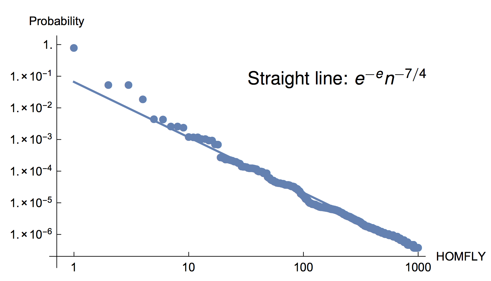
Knot types of 10 million 60-gons

Frequency plot of the HOMFLY polynomials produced by sampling 10 million random 60-gons (there were a total of 6371 distinct HOMFLYs).

cf. Baiesi–Orlandini–Stella

An explicit grid on the moment polytope

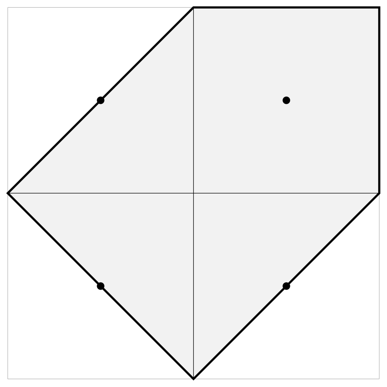
If we round every point \((d_1),\ldots , d_{n-3})\) in the moment polytope to the nearest point with half-integer coordinates \(\frac{1}{2}(x_1, \ldots , x_{n-3})\) …

Orthoscheme decomposition

… and subdivide the regions of attraction by

ordering and sign of \(d_i - \frac{1}{2} x_i\), we get a collection of identical, orthogonal simplices of equal area (this works for any \(n\)):

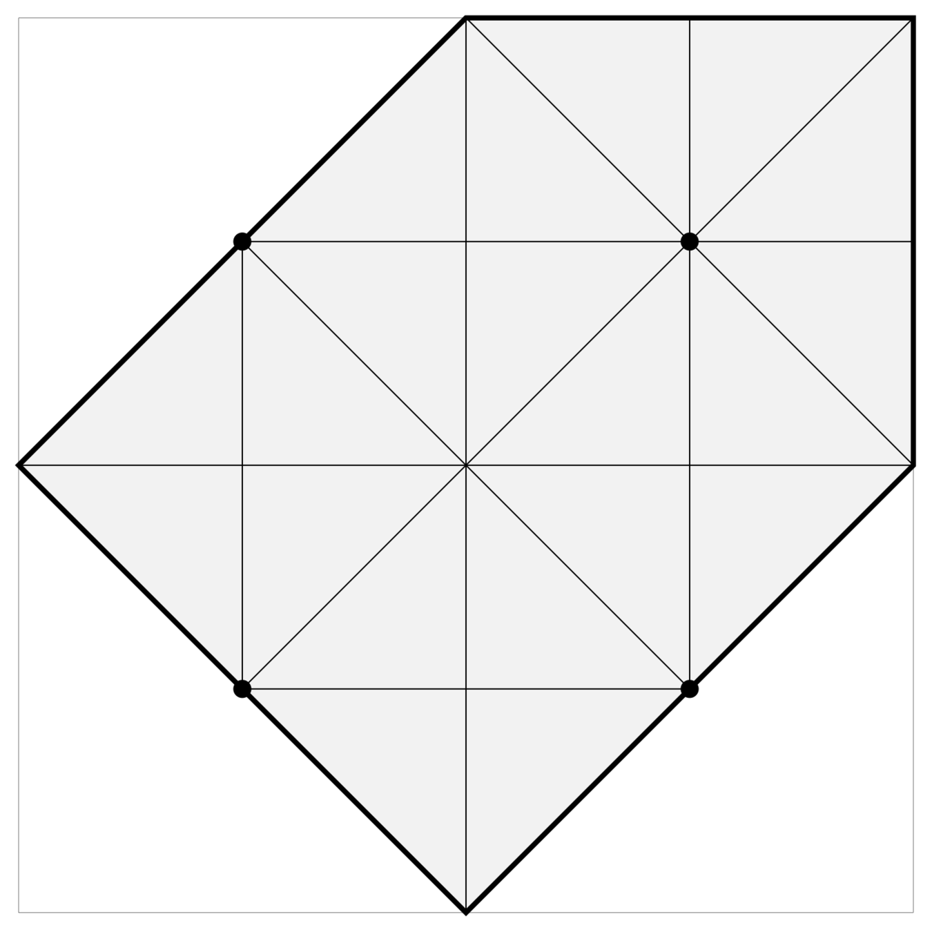
There are lots of simplices…

Proposition*: The number of half-integer points in \(\mathcal{P}_n\) is the Motzkin number

M_{n-3} = \sum_{k=0}^{\lfloor \frac{n-2}{2}\rfloor} \binom{n-2}{2k} C_k

\sim \sqrt{3} \frac{1 + \frac{1}{16(n-3)}}{(2n-3)\sqrt{(n-1)\pi}} 3^{n-2}

Therefore, there are exponentially many simplices in this decomposition. ☹️

… clever data structures to the rescue

Theorem (K. Chapman, in progress): With \(O(n^3)\) preprocessing of the transition probabilities, a direct sampling algorithm for equilateral \(n\)-gons in \(O(n^2 (\log n)^2)\) time.

The simplices are indexed by certain permutations.

One can recursively construct Lehmer codes of valid permutations using a Markov chain.

Question

What’s the corresponding story for planar \(n\)-gons? Or \(n\)-gons in \(\mathbb{R}^d\)?

The space of planar \(n\)-gons up to translation and rotation is \((n-3)\)-dimensional, so there is no chance of a symplectic structure.

Proposition: The space of \(n\)-gons in \(\mathbb{R}^d\) is the quotient of (almost all) of the space \((S^{d-1})^n\) by the (diagonal) action of the Möbius group.

Current Project: Use this structure to provide robust coordinates for polygons in all dimensions.

Question: Can this be adapted to give an algorithm for sampling the natural probability measure on \(n\)-gons?

Thank you!

References

The symplectic geometry of closed equilateral random walks in 3-space

J. Cantarella & C. Shonkwiler

Annals of Applied Probability 26 (2016), no. 1, 549–596

A fast direct sampling algorithm for equilateral closed polygons

J. Cantarella, B. Duplantier, C. Shonkwiler, & E. Uehara

Journal of Physics A 49 (2016), no. 27, 275202

J. Phys. A Highlight of 2016

Sampling knots using orthoschemes

K. Chapman

In preparation

Funding: Simons Foundation