Some Applications of Symplectic Geometry

Clayton Shonkwiler

Colorado State University

shonkwiler.org

/usna21

this talk!

Take-Home Message

Symplectic geometry can sound scary, but it turns out to be useful in some surprising contexts.

Symplecti-wha?

—Dusa McDuff & Dietmar Salamon

Introduction to Symplectic Topology

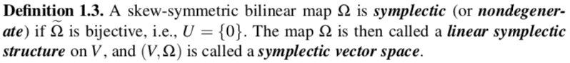
—Ana Cannas da Silva

Lectures on Symplectic Geometry

(\textcolor{12a4b6}{M},\textcolor{d9782d}{\omega})

A nice space, where multivariable calculus makes sense. Think spheres, tori, projective spaces, …

A rule for assigning a number to pairs of tangent vectors which transforms like (signed) area of the parallelogram they span.

\omega(v_1,v_2) = 1

\omega(v_1,v_2) = -1

v_1

v_2

Symplectic Manifold

Must be closed (think: divergence-free) and non-degenerate (doesn’t annihilate any vector).

Standard Example and Some Non-Examples

Example: \((\mathbb{R}^2,dx \wedge dy) = (\mathbb{C},\frac{i}{2}dz \wedge d\bar{z})\)

dx \wedge dy \left( \textcolor{12a4b6}{a \frac{\partial}{\partial x} + b \frac{\partial}{\partial y}}, \textcolor{d9782d}{c \frac{\partial }{\partial x} + d \frac{\partial}{\partial y}} \right) = ad - bc

(a,b) = a \vec{e}_1 + b \vec{e}_2 = a \frac{\partial}{\partial x} + b \frac{\partial}{\partial y}

(c,d) = c \vec{e}_1 + d \vec{e}_2 = c \frac{\partial}{\partial x} + d \frac{\partial}{\partial y}

Non-Example: \((\mathbb{R}^3, dx \wedge dy)\)

For any vector \(v\), \(dx \wedge dy\left(\frac{\partial}{\partial z}, v\right) = 0\), so \(dx \wedge dy\) is degenerate.

Non-Example: \((\mathbb{R}^4, dx_1 \wedge dy_1 + y_1 dx_2 \wedge dy_2)\)

Because of the coefficient \(y_1\), this is not closed (“not divergence-free”).

Examples

\((S^2,d\theta\wedge dz)\)

\((\mathbb{R}^2,dx \wedge dy) = (\mathbb{C},\frac{i}{2}dz \wedge d\bar{z})\)

\((S^2,\omega)\), where \(\omega_p(u,v) = (u \times v) \cdot p\)

\((\mathbb{R}^2,\omega)\) where \(\omega(u,v) = \langle i u, v \rangle \)

\((\mathbb{C}^n, \frac{i}{2} \sum dz_k \wedge d\overline{z}_k)\)

\((\mathbb{C}^{m \times n}, \omega)\) with \(\omega(X_1,X_2) = -\operatorname{Im} \operatorname{trace}(X_1^* X_2)\).

\((T^* \mathbb{R}^n,\sum dq_i \wedge dp_i)\)

phase space

position

momentum

What does this get you?

Volume

\(\omega^{\wedge n} = \omega \wedge \dots \wedge \omega\) is a volume form on \(M\), and induces a measure

m(U) := \int_U \omega^{\wedge n}

called Liouville measure on \(M\).

In particular, if \(M\) is compact, this can be normalized to give a probability measure.

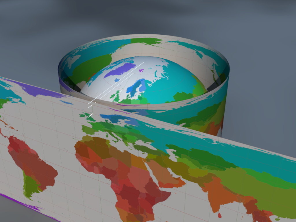
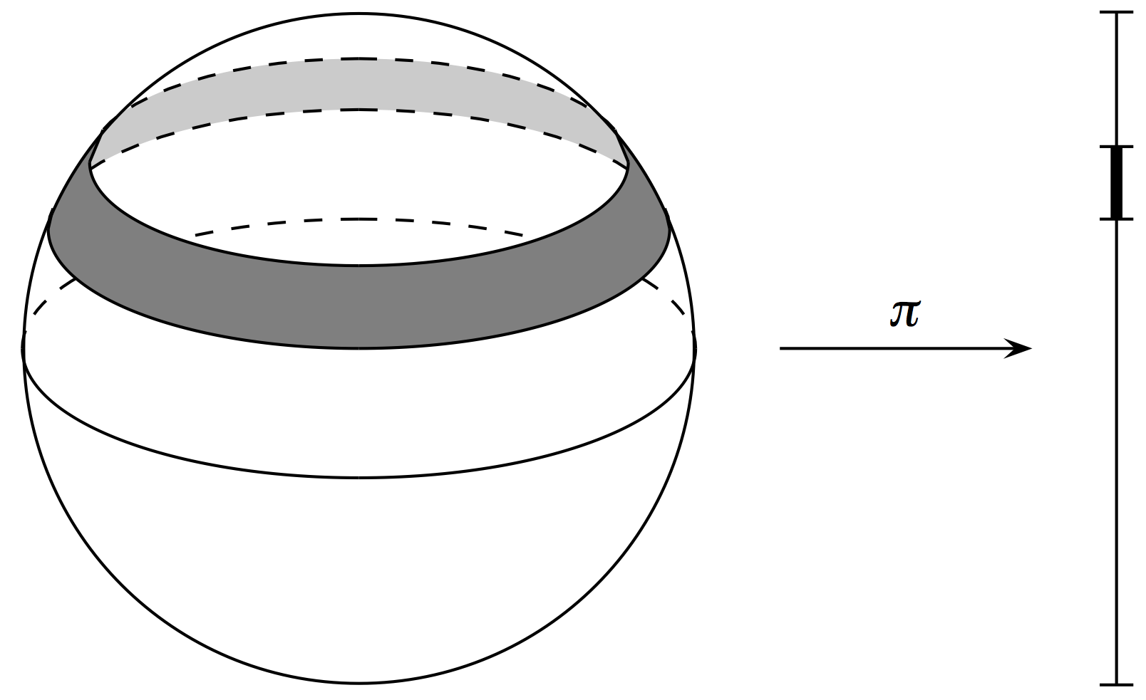
Theorem [Archimedes]

\(\mathrm{d}\theta \wedge \mathrm{d}z\) is the standard area form on the unit sphere \(S^2\).

\int_{S^2} \mathrm{d}\theta \wedge \mathrm{d}z = \int_{-1}^1 \int_0^{2\pi} \mathrm{d}\theta\, \mathrm{d}z = 4\pi

A (Very) Classical Example

KoenB [ ] from Wikimedia Commons

Hamiltonian Mechanics

“Evolution of a physical system follows the symplectic gradient”

Functions and Symplectic Gradients

If \(H: M \to \mathbb{R}\) is smooth, then there exists a unique vector field \(X_H\) so that \({dH = \iota_{X_H}\omega}\), i.e.,

dH(\cdot) = \omega(X_H, \cdot)

(\(X_H\) is called the Hamiltonian vector field for \(H\), or sometimes the symplectic gradient of \(H\))

Example. \(H: (S^2, d\theta\wedge dz) \to \mathbb{R}\) given by \(H(\theta,z) = z\).

\(dH = dz = \iota_{\frac{\partial}{\partial \theta}}(d\theta\wedge dz)\), so \(X_H = \frac{\partial}{\partial \theta}\).

\(H\) is constant on orbits of \(X_H\):

\(\mathcal{L}_{X_H}(H) = dH(X_H)=\omega(X_H,X_H) = 0\)

Some Mechanics

Suppose we have a particle of mass \(m\) with position \(\vec{q} = (q_1,q_2,q_3)\).

Suppose the particle is subject to a potential \(V(\vec{q})\).

Newton’s Second Law: \(-\nabla V(\vec{q}) = m \frac{d^2 \vec{q}}{dt^2}\).

Momenta \(p_i := m \frac{dq_i}{dt}\).

\((\vec{q},\vec{p})\in T^*\mathbb{R}^3 \cong \mathbb{R}^6\); canonical symplectic form \(\omega = dq_1 \wedge dp_1 + dq_2 \wedge dp_2 + dq_3 \wedge dp_3\).

The Hamiltonian Formulation

Energy function (or Hamiltonian)

\(H(\vec{q},\vec{p}) := \frac{1}{2m}|\vec{p}|^2 + V(\vec{q})\).

\(dH = \sum\left(\frac{\partial H}{\partial p_i} dp_i + \frac{\partial H}{\partial q_i}dq_i\right)\),

\((\vec{q}(t),\vec{p}(t))\) is an integral curve for \(X_H\) if and only if

\(\frac{dq_i}{dt} = \frac{\partial H}{\partial p_i} = \frac{1}{m} p_i\)

\(\frac{dp_i}{dt} = -\frac{\partial H}{\partial q_i} = -\frac{\partial V}{\partial q_i}.\)

This is Newton’s Second Law written as a first-order system!

\(X_H = \sum\left(\frac{\partial H}{\partial p_i} \frac{\partial}{\partial q_i} - \frac{\partial H}{\partial q_i} \frac{\partial}{\partial p_i}\right)\).

Noether’s Theorem

“Every continuous symmetry has a corresponding conserved quantity”

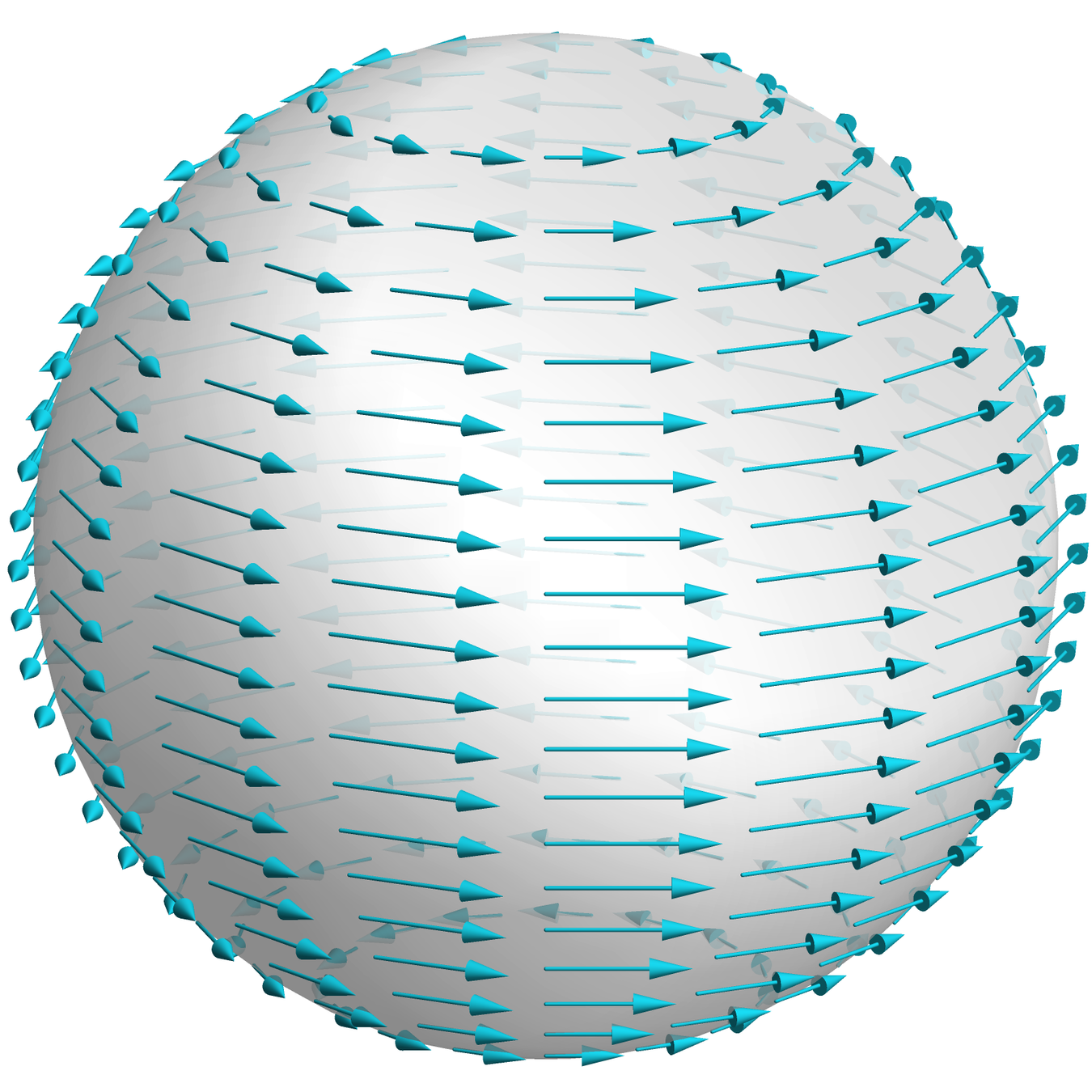
Circle Actions

A circle action on \((M,\omega)\) determines a vector field \(X\) by

X(p) = \left.\frac{d}{dt}\right|_{t=0}e^{i t} \cdot p

\(S^1=U(1)\) acts on \((S^2,d\theta \wedge dz)\) by

e^{it} \cdot(\theta, z) = (\theta + t, z).

So \(X = \frac{\partial}{\partial \theta}\).

Symmetries and Conserved Quantities

Definition. A circle action on \((M,\omega)\) is Hamiltonian if there exists a map

\mu: M \to \mathbb{R}

so that \(d\mu = \iota_{X}\omega = \omega(X,\cdot)\), where \(X\) is the vector field generated by the circle action. In other words, \(X = X_\mu\).

\(X = \frac{\partial}{\partial \theta}\)

\(\mu(\theta,z) = z\)

\(\iota_X\omega = \iota_{\frac{\partial}{\partial \theta}} d\theta \wedge dz = (d\theta \wedge dz)\left(\frac{\partial}{\partial \theta},\cdot \right) = dz \)

Generalizing Archimedes

Theorem [Atiyah and Guillemin–Sternberg]

If \((M,\omega)\) is symplectic and \(\mathbb{T}=(S^1)^k\) acts in a Hamiltonian fashion, the conserved quantities are recorded by \(\mu:M \to \mathbb{R}^k\) with:

The level sets of \(\mu\) are connected.
\(\mu(M)\) is the convex hull of the images of the fixed points of the \(\mathbb{T}\) action.

Theorem [Duistermaat–Heckman]

If \(\dim(M)=2n\) and \(\dim(\mathbb{T})=k\), then the pushforward measure on the moment polytope \(\mu(M)\) is absolutely continuous w.r.t. Lebesgue measure, with continuous, piecewise-polynomial density of degree \(\leq n-k\).

In particular, if \(n=k\), then the pushforward measure is a constant multiple of Lebesgue measure.

Example

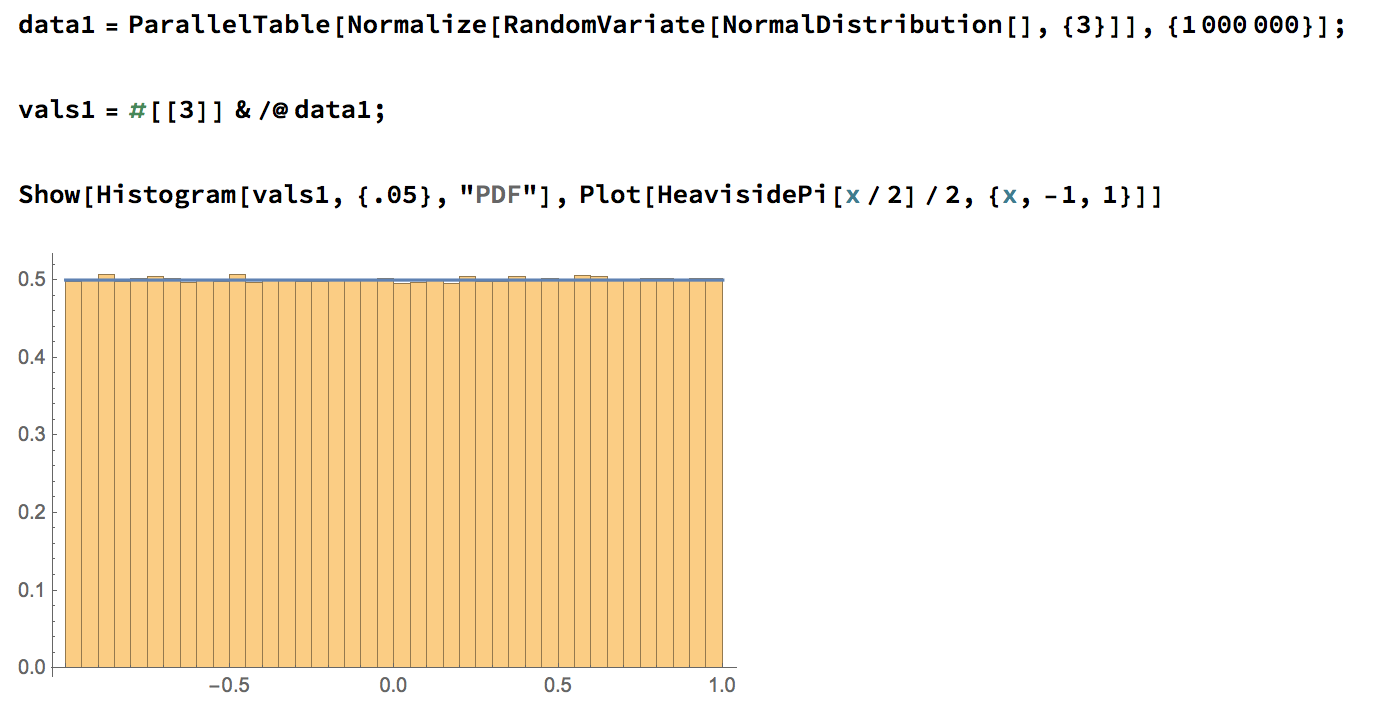
Theorem (Archimedes)

Let \(\mu: S^2 \to \mathbb{R}\) be given by \(\mu(x,y,z) = z\). Pushing forward the uniform measure on \(S^2\) to the image \([-1,1]\) gives Lebesgue measure.

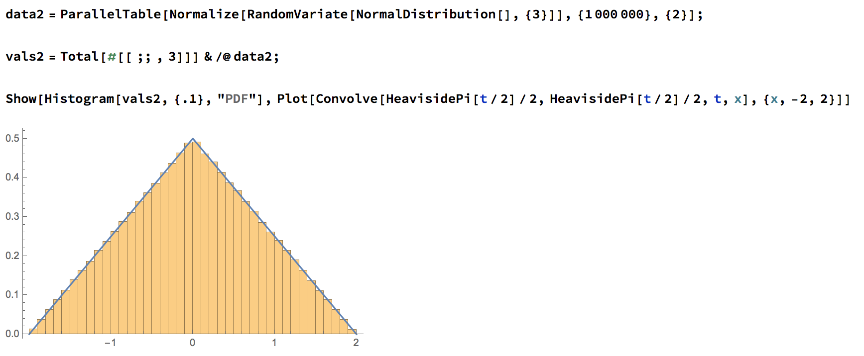
Example 2

Proposition. If we rotate both factors of \(S^2 \times S^2\) simultaneously around the \(z\)-axis, the moment map is \(((x_1,y_1,z_1),(x_2,y_2,z_2))\mapsto z_1 + z_2\), and the pushforward measure on \([-2,2]\) has density given by the triangle function.

Complex Example

The \(\mathbb{T}^2 = U(1) \times U(1)\) action on \(\mathbb{CP}^2\) given by

(e^{i\theta_1},e^{i\theta_2})\cdot [z_0:z_1:z_2] = \left[z_0:e^{i\theta_1}z_1:e^{i\theta_2}z_2\right]

has moment map

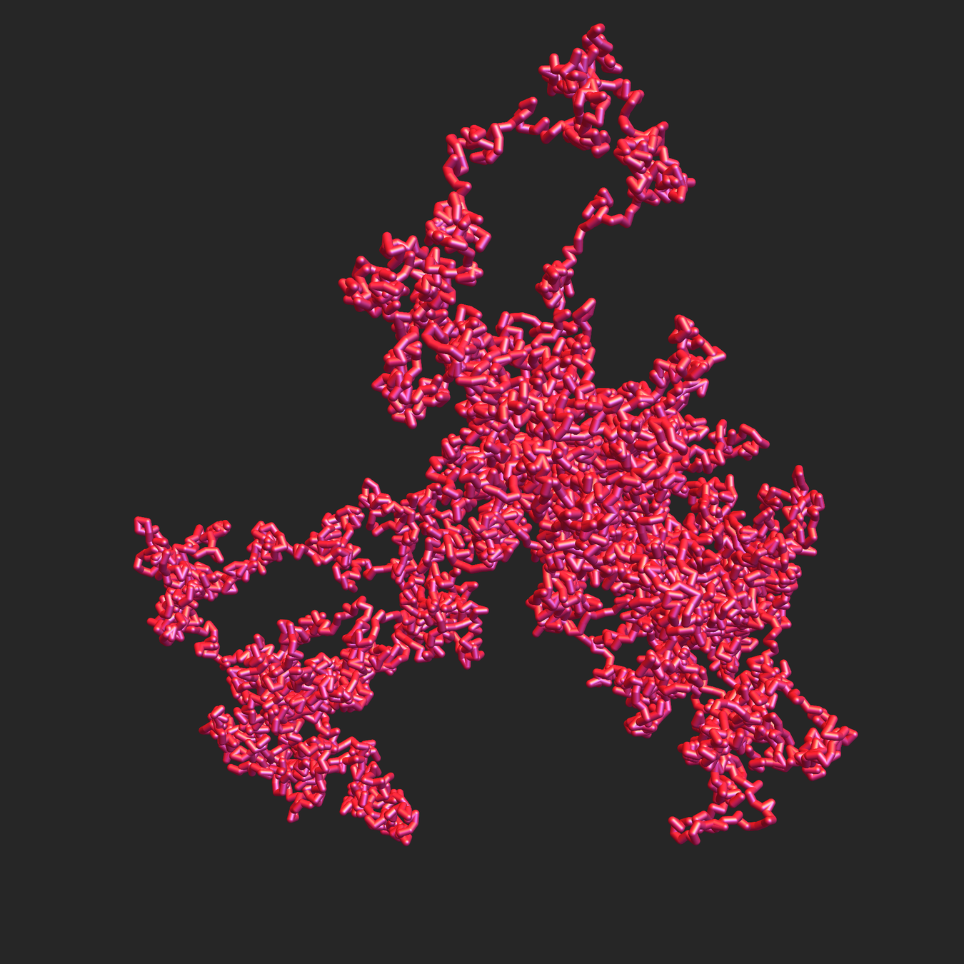
\mu([z_0:z_1:z_2]) = -\frac{1}{2} \left(\frac{|z_1|^2}{|z_0|^2+|z_1|^2+|z_2|^2},\frac{|z_2|^2}{|z_0|^2+|z_1|^2+|z_2|^2}\right).

Application to Polymers

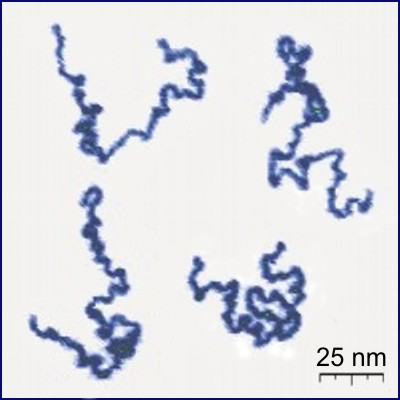
In solution, linear polymers become crumpled:

Protonated P2VP

Roiter–Minko, J. Am. Chem. Soc. 127 (2005), 15688-15689

[CC BY-SA 3.0], from Wikimedia Commons

Modern polymer physics is based on the analogy between a polymer chain and a random walk.

— Alexander Grosberg

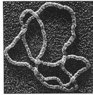
Ring Polymers

Wassermann et al. Science 229 (1985), 171–174

Lots of Symmetries!

Continuous symmetry \(\Rightarrow\) conserved quantity

The space of equilateral \(n\)-gons has lots of symmetries...

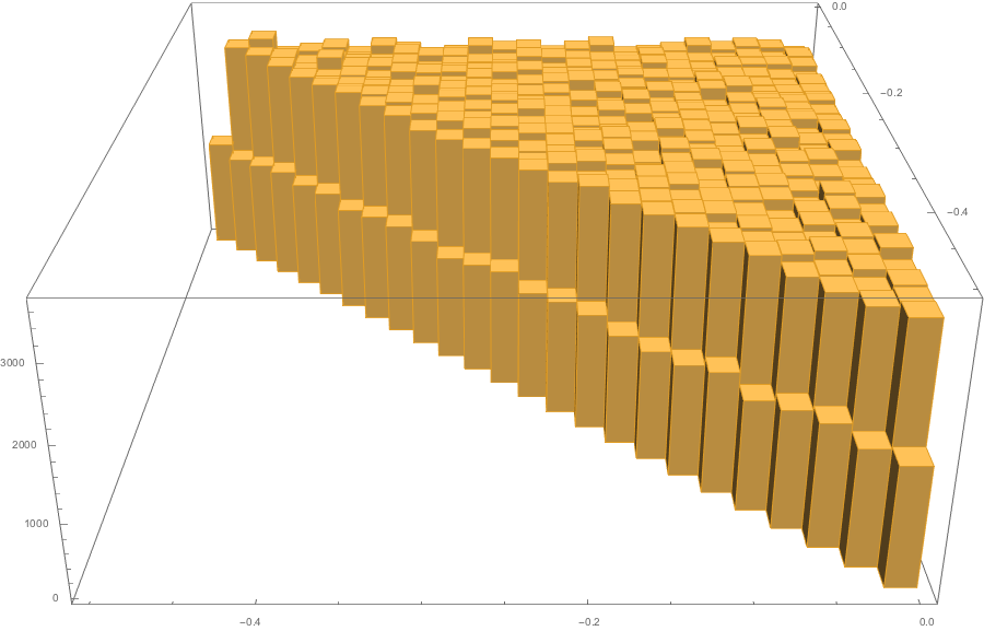
A Generalized Archimedes Theorem

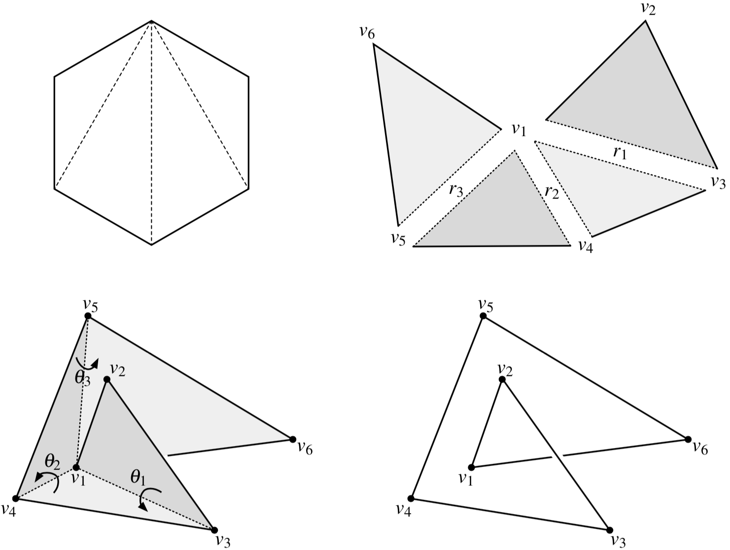
Theorem [with Cantarella]

The standard volume form on polygon space is

\(\mathrm{d}\theta_1 \wedge \dots \wedge \mathrm{d}\theta_{n-3} \wedge \mathrm{d} r_1 \wedge \dots \wedge \mathrm{d}r_{n-3}\)

Corollary [with Cantarella, Duplantier, Uehara]

The first efficient, provably correct algorithm for sampling equilateral random polygons in \(\mathbb{R}^3\).

Application to Frame Theory

Signal: \(v \in \mathbb{C}^d\)

Design: \(f_1, \dots , f_n \in \mathbb{C}^d\)

Measurements: \(\langle f_1, v \rangle, \dots , \langle f_n, v \rangle \).

Parseval’s Theorem

If \(f_1, \dots , f_d \in \mathbb{C}^d\) is an orthonormal basis,

\(\|v\|^2 = \sum |\langle f_i, v \rangle |^2 = \|F^* v\|^2\)

for any \(v \in \mathbb{C}^d\).

Even better,

\(v = \sum \langle f_i, v \rangle f_i = FF^* v \).

If \(F = [f_1 \, f_2 \dots f_n]\), the measurement vector is \(F^*v\).

\(\Leftrightarrow FF^* = \mathrm{Id}_{d \times d}\)

Parseval frame

Fact: For any \(n \geq d\), there exist Parseval frames \(f_1, \dots , f_n \in \mathbb{C}^d\) so that \(\|f_i\|=\|f_j\|\) for all \( i,j\); these are the equal-norm Parseval frames (ENPs).

This is fragile! What if a measurement gets lost?

Group Actions on Frames

Some nice group actions on \(\mathbb{C}^{d \times n}\):

\(U(d)\) acts on the left
\(U(n)\) acts on the right
\(U(1)^d\) acts on the left
\(U(1)^n\) acts on the right

\mu_{U(d)}(F) = FF^*

\mu_{U(n)}(F) = -F^*F

\mu_{U(1)^d}\left(\begin{bmatrix} \rule[.8mm]{4mm}{.5px}\, f^1 \rule[.8mm]{4mm}{.5px}\\ \vdots \\ \rule[.8mm]{4mm}{.5px}\, f^d \rule[.8mm]{4mm}{.5px} \end{bmatrix}\right) = \left(\frac{1}{2}\|f^1\|^2 , \dots , \frac{1}{2}\|f^d\|^2\right)

\mu_{U(1)^n} \left(\begin{bmatrix} f_1 | \cdots | f_n \end{bmatrix}\right) = \left(-\frac{1}{2}\|f_1\|^2 , \dots , -\frac{1}{2}\|f_n\|^2\right)

Parseval frames

\(\mu_{U(d)}^{-1}(I_{d\times d})\)

equal-norm frames

\(\mu_{U(1)^N}^{-1}\left(-\frac{1}{2}r,\dots , -\frac{1}{2}r\right)\)

ENPs: \(\mu_{U(d)}^{-1}(I_{d \times d}) \cap \mu_{U(1)^n}^{-1}\left(-\frac{d}{2n}, \dots , -\frac{d}{2n}\right)\)

A Generalization of the Frame Homotopy Conjecture

Theorem [with Needham]

There is a continuous interpolation between any two frames \(f_1, \dots , f_n\) and \(g_1, \dots , g_n\) with \(FF^* = GG^*\) and \(\|f_i\| = \|g_i\|\) preserving these conditions.