EnsLoss: Stochastic Calibrated Loss Ensembles for Preventing Overfitting in Classification
Ben Dai (CUHK)
IMS-APRM 2026
Background
The objective of binary classification is to categorize each instance into one of two classes.
- Data: \( \mathbf{X} \in \mathbb{R}^d \to Y \in \{-1,+1\} \)
- Classifier: \( f(\mathbf{X}): \mathbb{R}^d \to \mathbb{R} \)
- Predicted label: \( \widehat{Y} = \text{sgn}(f(\mathbf{X})) \)
- Evaluation via Misclassification error (risk):
where \(\mathbf{1}(\cdot)\) is an indicator function.
Aim. To obtain the Bayes classifier or the best classifier:
$$R(\hat{f}_n) \to R(f^*) \quad f^* := \argmin R(f)$$
$$R(f) = 1 - \text{Acc}(f) = \mathbb{E}( \mathbf{1}(Y f(\mathbf{X}) \leq 0) ),$$
Background
Due to the discontinuity of the indicator function:
$$R(f) = 1 - \text{Acc}(f) = \mathbb{E}( \mathbf{1}(Y f(\mathbf{X}) \leq 0) ),$$
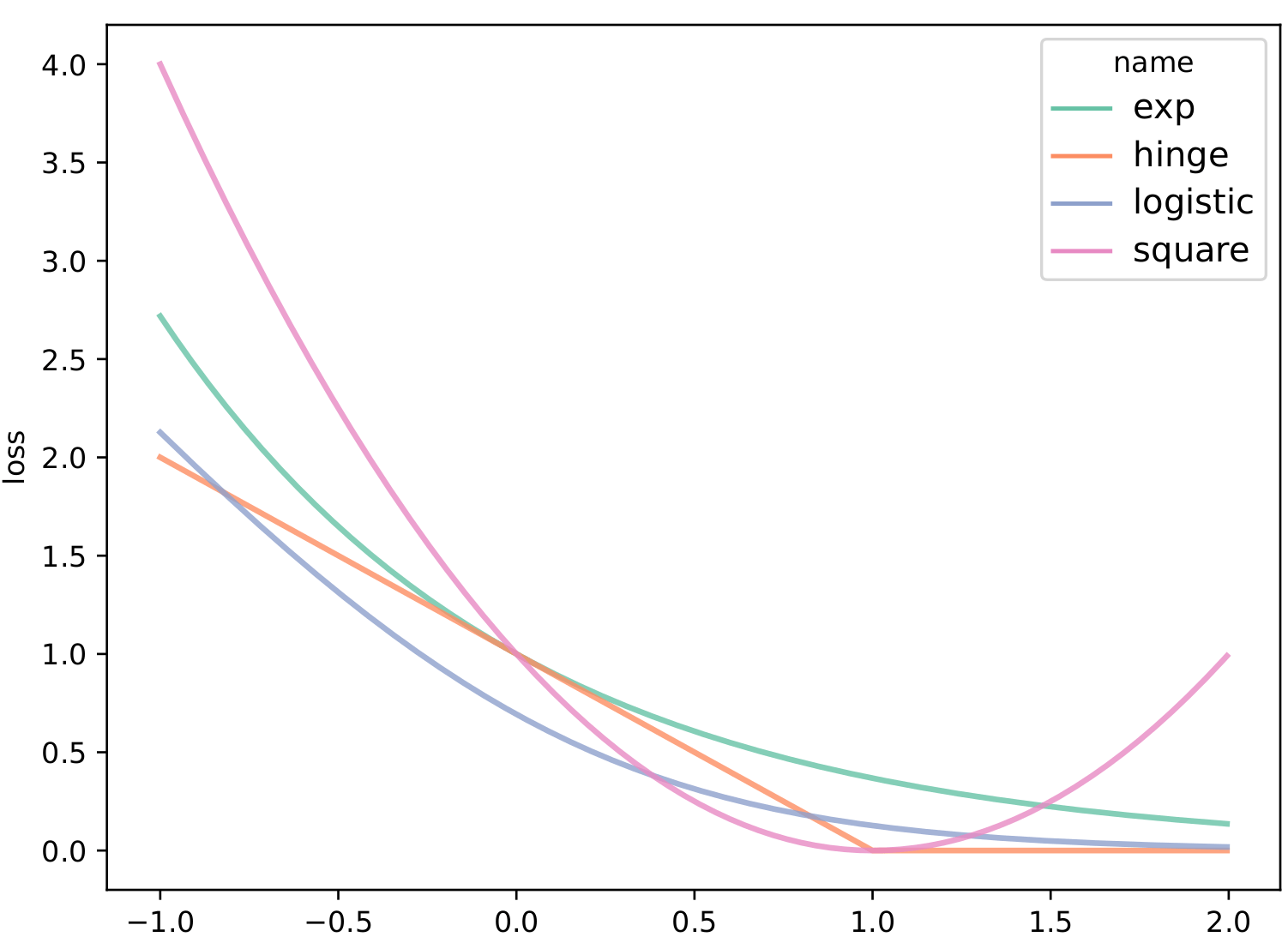
the zero-one loss is usually replaced by a convex and classification-calibrated loss \(\phi\) to facilitate the empirical computation (Lin, 2004; Zhang, 2004; Bartlett et al., 2006):
$$ R_{\phi}(f) = \mathbb{E}( \phi(Y f(\mathbf{X})) ) $$
For example, the hinge loss for SVM, exponential loss for AdaBoost, and logistic loss for logistic regression all follow this framework.
Background
Due to the discontinuity of the indicator function:
$$R(f) = 1 - \text{Acc}(f) = \mathbb{E}( \mathbf{1}(Y f(\mathbf{X}) \leq 0) ),$$
(If we optimize with respect to \(\phi\), will the resulting solution still be the function \(f^*\) that we need?)
That's why we need the loss \(\phi\) to be calibrated/consistent?
the zero-one loss is usually replaced by a convex and classification-calibrated loss \(\phi\) to facilitate the empirical computation (Lin, 2004; Zhang, 2004; Bartlett et al., 2006):
$$ R_{\phi}(f) = \mathbb{E}( \phi(Y f(\mathbf{X})) ) $$
For example, the hinge loss for SVM, exponential loss for AdaBoost, and logistic loss for logistic regression all follow this framework.
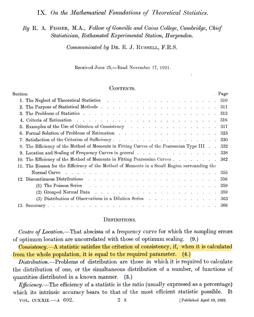
Fisher Consistency
A portrait of Sir Ronald Aylmer Fisher. Image from the MacTutor History of Mathematics Archive.
The cover page of Ronald A. Fisher (1922), where definition of consistency is provided.
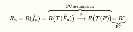
Fisher Consistency
(ERM via a surrogate loss).
- Obtain \( \hat{f} \) from a ERM with a surrogate loss (\( \hat{\delta} = \mathbb{I}(\hat{f} \geq 0) \))
$$ \hat{f}_{\phi} = \argmin_f \mathbb{E}_n \phi\big(Y f(\mathbf{X}) \big) $$
$$Acc \big ( \hat{\delta}(F_n) \big) \xrightarrow{\mathbb{P}} Acc \big( \delta(F) \big) = \max_{\delta} Acc(\delta)$$
Fisher Consistency
(ERM via a surrogate loss).
- Obtain \( \hat{f} \) from a ERM with a surrogate loss (\( \hat{\delta} = \mathbb{I}(\hat{f} \geq 0) \))
$$ \hat{f}_{\phi} = \argmin_f \mathbb{E}_n \phi\big(Y f(\mathbf{X}) \big) $$
$$ f_\phi = \argmin_f \mathbb{E} \phi\big(Y f(\mathbf{X}) \big)$$
$$Acc \big ( \hat{\delta}(F_n) \big) \xrightarrow{\mathbb{P}} Acc \big( \delta(F) \big) = \max_{\delta} Acc(\delta)$$
FC leads to conditions for "consistent" surrogate losses
(If we optimize with respect to \(\phi\), will the resulting solution still be the function \(f^*\) that we need?)
FC: The population minimizer of \(R_\phi\) also minimizes \(R\)
Fisher Consistency
Definition 1 (Bartlett et al. (2004)). A loss function \(\phi(\cdot)\) is classification-calibrated, if for every sequence of measurable function \(f_n\) and every probability distribution on \( \mathcal{X} \times \{\pm 1\}\),
$$R_{\phi}(f_n) \to \inf_{f} R_{\phi}(f) \ \text{ implies that } \ R(f_n) \to \inf_{f} R(f).$$
A calibrated loss function \(\phi\) guarantees that any sequence \(f_n\) that optimizes \(R_\phi\) will eventually also optimize \(R\), thereby ensuring consistency in maximizing classification accuracy.
A series of studies (Lin, 2001; Zhang, 2004; Bartlett et al., 2004) culminates in the following theorem for iff conditions of FC:
Fisher Consistency
Fisher Consistency
A series of studies (Lin, 2001; Zhang, 2004; Bartlett et al., 2004) culminates in the following theorem for iff conditions of FC:
Theorem 3.1 in Lin. (2001) (informal) Consider a loss function \(\phi\) satisfying the following conditions:
$$(1) \quad \phi(z) < \phi(-z), \forall z >0; \qquad (2) \quad \phi'(z) \neq 0 \text{ exits}.$$
Then \(\phi\) is Fisher consistent.
Fisher Consistency
Theorem 3.1 in Lin. (2001) (informal) Consider a loss function \(\phi\) satisfying the following conditions:
$$(1) \quad \phi(z) < \phi(-z), \forall z >0; \qquad (2) \quad \phi'(z) \neq 0 \text{ exits}.$$
Then \(\phi\) is Fisher consistent.
(A closely related version appears as Theorem 4.1 in Zhang, 2004.)
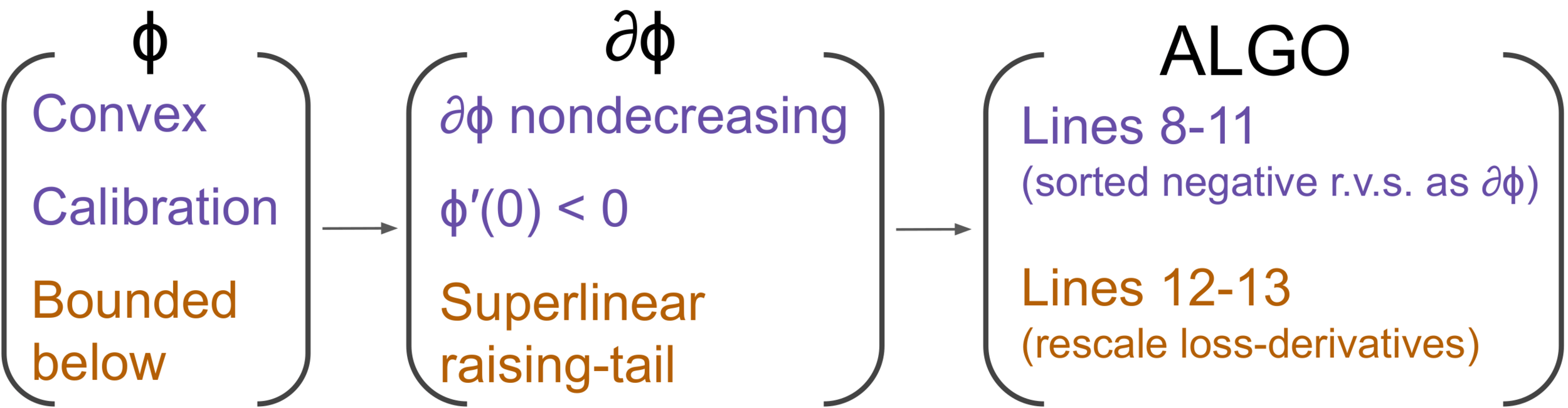
Theorem 2 in Bartlett et al. (2004) (informal) Let \(\phi\) be convex. Then \(\phi\) is consistency iff it is differentiable at 0 and \(\phi'(0) < 0\).
A series of studies (Lin, 2001; Zhang, 2004; Bartlett et al., 2004) culminates in the following theorem for iff conditions of FC:
Fisher Consistency
Theorem 3.1 in Lin. (2001) (informal) Consider a loss function \(\phi\) satisfying the following conditions:
$$(1) \quad \phi(z) < \phi(-z), \forall z >0; \qquad (2) \quad \phi'(z) \neq 0 \text{ exits}.$$
Then \(\phi\) is Fisher consistent.
(A closely related version appears as Theorem 4.1 in Zhang, 2004.)
Theorem 2 in Bartlett et al. (2004) (informal) Let \(\phi\) be convex. Then \(\phi\) is consistency iff it is differentiable at 0 and \(\phi'(0) < 0\).
A series of studies (Lin, 2001; Zhang, 2004; Bartlett et al., 2004) culminates in the following theorem for iff conditions of FC:
FC in Multiclass. Lee, Lin and Wahba (2012); Liu (2007); Zou, Zhu and Hastie (2008)
Classification ERM framework
(i) Select a convex and calibrated (CC) loss function \(\phi\)
Classification ERM framework
$$ \widehat{f}_{n} = \argmin_{f \in \mathcal{F}} \ \widehat{R}_{\phi} (f), \quad \widehat{R}_{\phi} (f) := \frac{1}{n} \sum_{i=1}^n \phi \big( y_i f(\mathbf{x}_i) \big).$$
(i) Select a convex and calibrated (CC) loss function \(\phi\)
(ii) Directly minimizes the ERM of \(R_\phi\) to obtain \(f_n\)
(SGD is widely adopted for its scalability and generalization when dealing with large-scale datasets and DL models)
$$\pmb{\theta}^{(t+1)} = \pmb{\theta}^{(t)} - \gamma \frac{1}{B} \sum_{i \in \mathcal{I}_B} \nabla_{\pmb{\theta}} \phi( y_{i} f_{\pmb{\theta}^{(t)}}(\mathbf{x}_{i}) )$$
$$= \pmb{\theta}^{(t)} - \gamma \frac{1}{B} \sum_{i \in \mathcal{I}_B} y_i \partial \phi( y_{i} f_{\pmb{\theta}^{(t)}}(\mathbf{x}_{i}) ) \nabla_{\pmb{\theta}} f_{\pmb{\theta}^{(t)}}(\mathbf{x}_{i}),$$
The ERM paradigm with calibrated losses, when combined with ML/DL models and optimized using SGD, has achieved tremendous success in numerous real-world applications.
Loss selection in Practice
However, in practical applications, determining which loss function performs better is a very challenging problem, as it is typically unknown and can vary across datasets.
| BCE > Hinge | Hinge > BCE | |
| ResNet34 | 3 | 42 |
| ResNet50 | 26 | 19 |
| VGG16 | 9 | 36 |
| VGG19 | 13 | 32 |
We examine two of the most popular losses: BCE and Hinge loss. We provide experimental results on 45 CIFAR2 datasets, which also confirms that the superiority of the loss function is not consistent across different models / datasets.
Current approaches in theoretical analysis include:
- Convergence rate of \(R_{\phi}(\hat{f}_n) \to R^*_{\phi}\)
- Excess risk bounds (how \(R_{\phi}(\hat{f}_n) \to R^*_{\phi}\) implies \(R(\hat{f}_n) \to R^*\))
Current limitations in theoretical analysis are:
- Rates are difficult to characterize under finite sample situations
- Most existing theories are distribution-free, whereas in practice data is given but its distribution is unknown
Ensemble idea
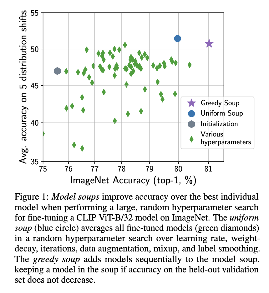
Mitchell, et al. "Model soups: averaging weights of multiple fine-tuned models improves accuracy without increasing inference time." ICML, 2022.
Ensemble idea
Mitchell, et al. "Model soups: averaging weights of multiple fine-tuned models improves accuracy without increasing inference time." ICML, 2022.
Limitation
-
Computational Intensity: Bagging requires training multiple base models (often hundreds), making it computationally expensive compared to single models.
-
Some methods require additional validation sets.
Let's Dropout!
Nitish, et al. "Dropout: a simple way to prevent neural networks from overfitting." JMLR, 2014
$$\pmb{\theta}^{(t+1)} = \pmb{\theta}^{(t)} - \gamma \frac{1}{B} \sum_{i \in \mathcal{I}_B} \nabla_{\pmb{\theta}} \phi( y_{i} f_{\pmb{\theta}^{(t)}}(\mathbf{x}_{i}) )$$
EnsLoss: Calibrated Loss Ensembles
Inspired by Dropout
(model ensemble over one training process)
$$\pmb{\theta}^{(t+1)} = \pmb{\theta}^{(t)} - \gamma \frac{1}{B} \sum_{i \in \mathcal{I}_B} \nabla_{\pmb{\theta}} \phi( y_{i} f_{\pmb{\theta}^{(t)}}(\mathbf{x}_{i}) )$$
EnsLoss: Calibrated Loss Ensembles
Inspired by Dropout
(model ensemble over one training process)
$$= \pmb{\theta}^{(t)} - \gamma \frac{1}{B} \sum_{i \in \mathcal{I}_B} \partial \phi( y_{i} f_{\pmb{\theta}^{(t)}}(\mathbf{x}_{i}) ) \nabla_{\pmb{\theta}} f_{\pmb{\theta}^{(t)}}(\mathbf{x}_{i}),$$
EnsLoss: Calibrated Loss Ensembles
$$\pmb{\theta}^{(t+1)} = \pmb{\theta}^{(t)} - \gamma \frac{1}{B} \sum_{i \in \mathcal{I}_B} \nabla_{\pmb{\theta}} \phi( y_{i} f_{\pmb{\theta}^{(t)}}(\mathbf{x}_{i}) )$$
$$= \pmb{\theta}^{(t)} - \gamma \frac{1}{B} \sum_{i \in \mathcal{I}_B} \partial \phi( y_{i} f_{\pmb{\theta}^{(t)}}(\mathbf{x}_{i}) ) \nabla_{\pmb{\theta}} f_{\pmb{\theta}^{(t)}}(\mathbf{x}_{i}),$$
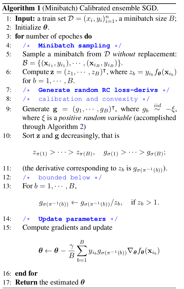
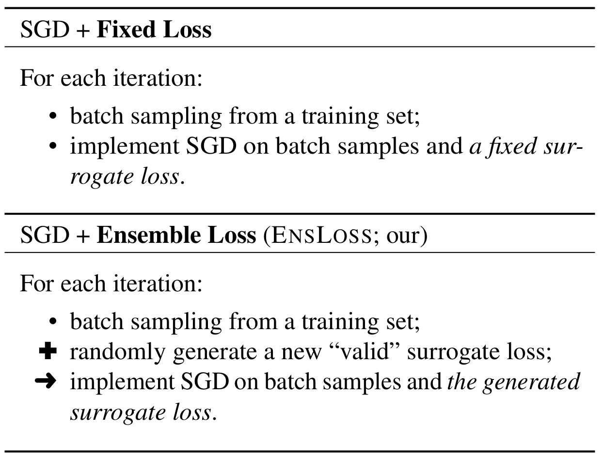
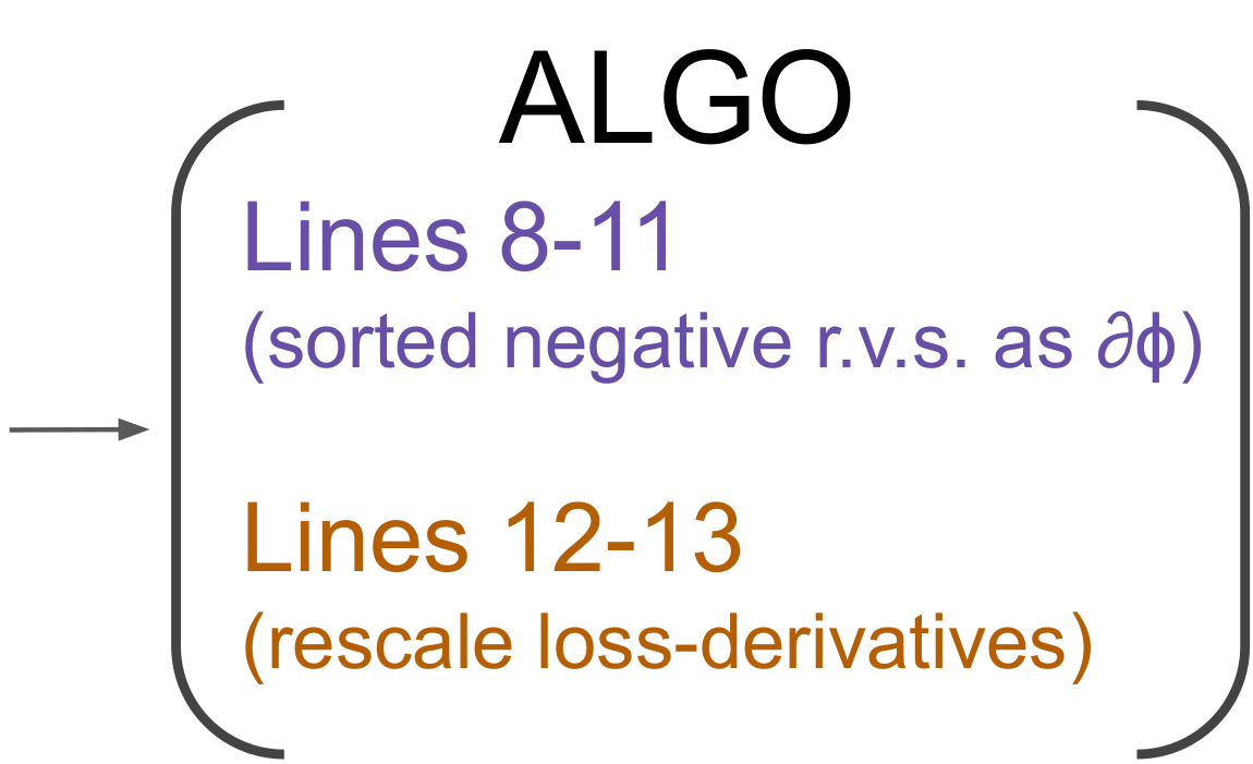
EnsLoss
Experiments
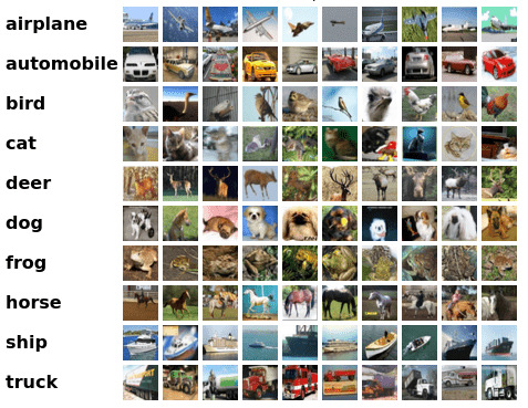
CIFAR
We construct binary CIFAR (CIFAR2), by selecting all possible pairs from CIFAR10, resulting:
10 x 9 / 2 = 45
CIFAR2 datasets.
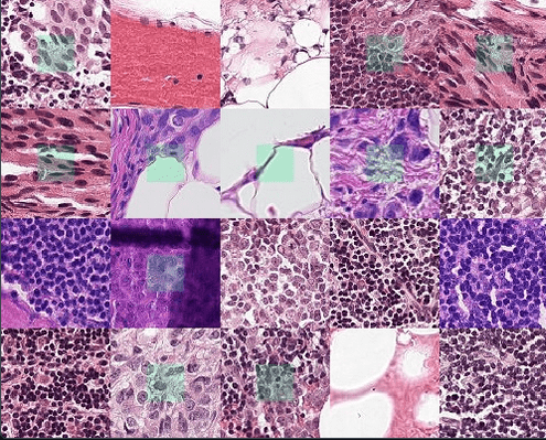
PCam
PCam is a binary image classification dataset comprising 327,680 96x96 images from histopathologic scans of lymph node sections
Experiments
OpenML

We applied a filering:
n >= 1000
d >= 1000
at least one official run
resulting 14 datasets

no dataset cherry pick
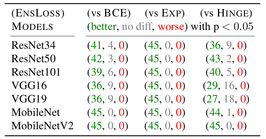
CIFAR2
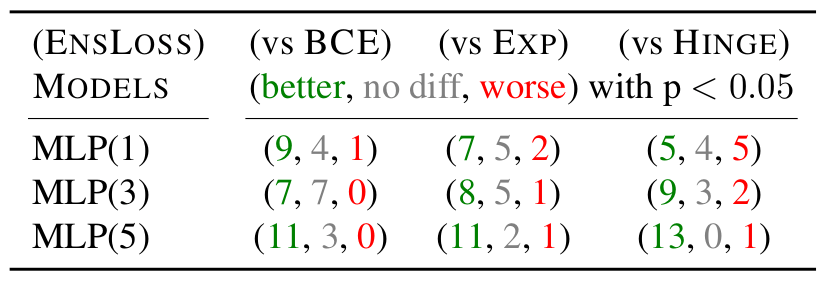
OpenML
PCam
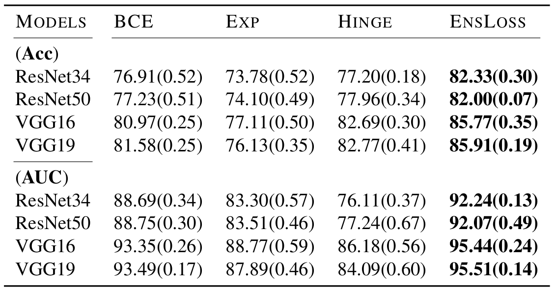
EnsLoss is a more desirable option compared to fixed losses in image data;
and it is a viable option worth considering in tabular data.
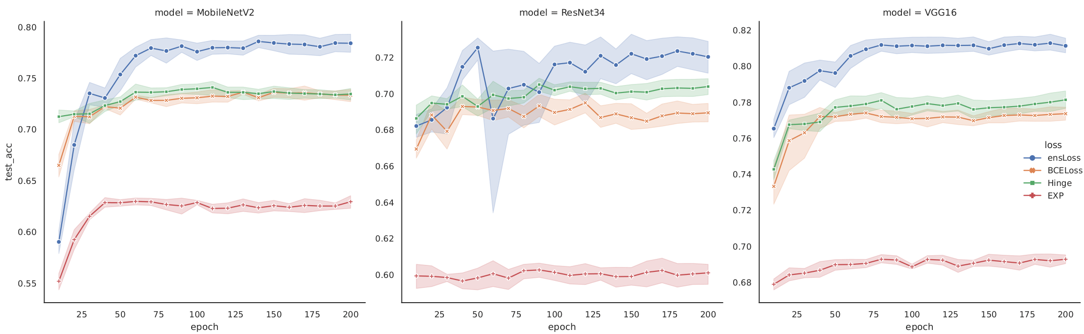
Epoch-level performance
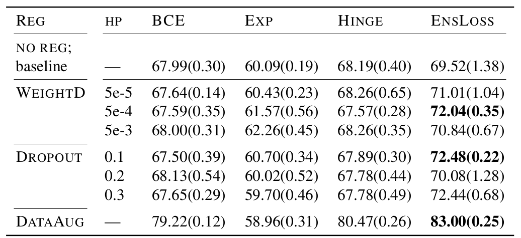
Compatibility of prevent-overfitting methods
EnsLoss consistently outperforms the fixed losses across epochs;
and it is compatible with other methods, and their combination yields additional improvement.
Summary
The primary motivation of EnsLoss behind consists of two components: “ensemble” and the “CC” of the loss functions.
Dai, B. (2025). EnsLoss: Stochastic Calibrated Loss Ensembles for Preventing Overfitting in Classification. ICML.
Thank you!