Regularized Composite ReLU-ReHU Loss Minimization with Linear Computation and Linear Convergence

Ben Dai (CUHK)

(Joint work with Yixuan Qiu)

SVM

• Support Vector Machines (SVMs) were introduced by Vapnik and Chervonenkis in the 1990s.

• SVM and Kernel SVM gained widespread popularity in the late 1990s and early 2000s, and impressive empirical performance across various applications.

• DBLP: SVM (11,350 matches); classification (158,937 matches)

• LIBSVM, developed by Lin in 2000, became the most widely-used SVM software.
  • downloaded millions of times

Source: https://stackoverflow.com/questions/73589036/clarity-needed-on-svm-concepts

LIBLINEAR

• LIBLINEAR is the winner of  ICML 2008 large-scale learning challenge (linear SVM track). It is also used for winning KDD Cup 2010.

• In scikit-learn, liblinear is the default solver for SVMs in Python.

LIBLINEAR

As indicated from the official Liblinear website, thanks to contributions from researchers and developers worldwide, Liblinear has incorporated interfaces for various languages:

{ R, Python, Matlab, Java, Perl, Ruby, and even PHP }

The popularity of Liblinear is thus evident.

LIBLINEAR

LIBLINEAR

LIBLINEAR

• From 2008 to 2025, a 17-year period of continuous contributions.

• Countless hours have been devoted.

• Since its development in 2008, it has consistently remained the No. 1 solver for solving SVMs.

Dual Coordinate Desent

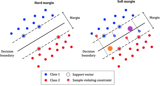
The primal is QP with 2n linear constraints

Given a training set of \(n\) points of the form \((\mathbf{x}_i, y_i)_{i=1}^n\), where \(y = \pm 1\) which indicates the binary label of the \(i\)-th instance \( \mathbf{x}_i \in \mathbb{R}^d \).

Primal form.

$$ \min_{\pmb{\beta}, \xi} \sum_{i=1}^{n} C_i \xi_i + \frac{1}{2} \| \pmb{\beta} \|^2 $$

$$y_i \pmb{\beta}^T \mathbf{x}_i \geq 1 - \xi_i, \quad \xi_i \geq 0$$

$$\min_{\pmb{\beta}} \sum_{i=1}^{n} C_i ( 1 - y_i \pmb{\beta}^T \mathbf{x}_i )_+ + \frac{1}{2} \| \pmb{\beta} \|^2 $$

After introducing slack variables,

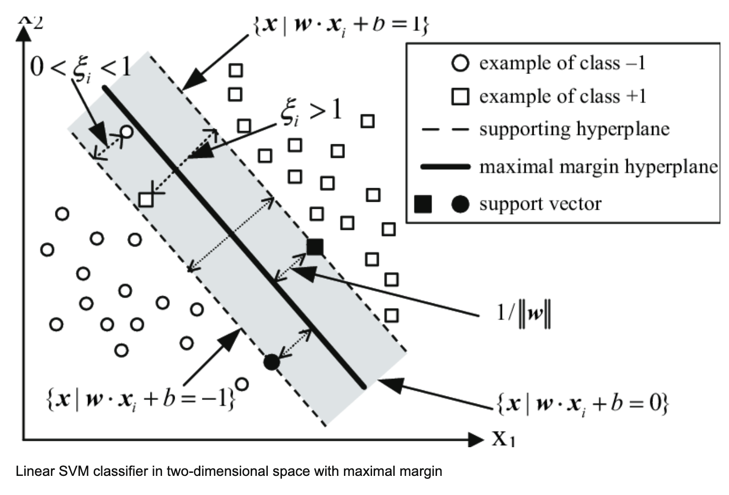
Source: https://www.researchgate.net/figure/Linear-SVM-classifier-in-two-dimensional-space-with-maximal-margin_fig1_221649317

Dual Coordinate Desent

The dual is a box-constrained QP

• simpler form than the primal problem
• naturally leads to coordinate descent (CD)

• Lagrange multiplier

$$L_P = \sum_{i=1}^{n} C_i \xi_i + \frac{1}{2} \| \pmb{\beta} \|^2  - \sum_{i=1}^n \alpha_i \big( y_i \mathbf{x}_i^T \pmb{\beta} - (1 - \xi_i) \big)  - \sum_{i=1}^n \mu_i \xi_i$$

• Taking derivatives to w.r.t. \( \pmb{\beta} \) and \( \xi_i \):

$$ \pmb{\beta} =  \sum_{i=1}^n \alpha_i y_i \mathbf{x}_i, \quad \alpha_i = C_i -  \mu_i, $$

Dual form:

$$ \min_{\pmb{\alpha}} \frac{1}{2} \pmb{\alpha}^T \mathbf{Q} \pmb{\alpha} - \mathbf{1}^T \pmb{\alpha}, \quad \text{s.t.} \quad 0 \leq \alpha_i \leq C_i$$

KKT Condition

where \( \mathbf{Q}_{ij} = y_i y_j \mathbf{x}^T_i \mathbf{x}_j \).

Dual Coordinate Desent

The dual is a box-constrained QP

• simpler form than the primal problem
• naturally leads to coordinate descent (CD)

Dual Coordinate Desent

$$ \min_{\delta_i} \frac{1}{2} Q_{ii} \delta_i^2 + \big((\mathbf{Q} \pmb{\alpha})_i - 1\big) \delta_i, \quad \text{s.t.} \quad -\alpha_i \leq \delta_i \leq C_i - \alpha_i$$

where \( \mathbf{Q}_{ij} = y_i y_j \mathbf{x}^T_i \mathbf{x}_j \). The solution to the sub-problem is:

CD sub-problem. Given an "old" value of \( \pmb{\alpha} \), we solve

$$ \delta^*_i = \max \Big( -\alpha_i, \min\big( C_i - \alpha_i, \frac{1 - ( (\mathbf{Q}\pmb{\alpha})_i )}{Q_{ii}}  \big) \Big)  $$

$$ \alpha_i^* \leftarrow  \alpha_i + \delta^*_i$$

Dual Coordinate Desent

$$ \min_{\delta_i} \frac{1}{2} Q_{ii} \delta_i^2 + \big((\mathbf{Q} \pmb{\alpha})_i - 1\big) \delta_i, \quad \text{s.t.} \quad -\alpha_i \leq \delta_i \leq C_i - \alpha_i$$

where \( \mathbf{Q}_{ij} = y_i y_j \mathbf{x}^T_i \mathbf{x}_j \). The solution to the sub-problem is:

CD sub-problem. Given an "old" value of \( \pmb{\alpha} \), we solve

$$ \delta^*_i = \max \Big( -\alpha_i, \min\big( C_i - \alpha_i, \frac{1 - ( (\mathbf{Q}\pmb{\alpha})_i )}{Q_{ii}}  \big) \Big)  $$

$$ \alpha_i^* \leftarrow  \alpha_i + \delta^*_i$$

Note that \( (\mathbf{Q} \mathbf{\alpha})_{i} = y_i \mathbf{x}_i^T \sum_{j=1}^n y_j \mathbf{x}_j \alpha_j \)

\( O(nd) \)

(at least O(n) if Q is pre-computed)

Dual Coordinate Desent

$$ \min_{\delta_i} \frac{1}{2} Q_{ii} \delta_i^2 + \big((\mathbf{Q} \pmb{\alpha})_i - 1\big) \delta_i, \quad \text{s.t.} \quad -\alpha_i \leq \delta_i \leq C_i - \alpha_i$$

where \( \mathbf{Q}_{ij} = y_i y_j \mathbf{x}^T_i \mathbf{x}_j \). The solution to the sub-problem is:

CD sub-problem. Given an "old" value of \( \pmb{\alpha} \), we solve

$$ \delta^*_i = \max \Big( -\alpha_i, \min\big( C_i - \alpha_i, \frac{1 - ( (\mathbf{Q}\pmb{\alpha})_i )}{Q_{ii}}  \big) \Big)  $$

$$ \alpha_i^* \leftarrow  \alpha_i + \delta^*_i$$

Note that \( (\mathbf{Q} \mathbf{\alpha})_{i} = y_i \mathbf{x}_i^T \sum_{j=1}^n y_j \mathbf{x}_j \alpha_j \)

\( O(nd) \)

(at least O(n) if Q is pre-computed)

Dual Coordinate Desent

$$ \min_{\delta_i} \frac{1}{2} Q_{ii} \delta_i^2 + \big((\mathbf{Q} \pmb{\alpha})_i - 1\big) \delta_i, \quad \text{s.t.} \quad -\alpha_i \leq \delta_i \leq C_i - \alpha_i$$

where \( \mathbf{Q}_{ij} = y_i y_j \mathbf{x}^T_i \mathbf{x}_j \). The solution to the sub-problem is:

CD sub-problem. Given an "old" value of \( \pmb{\alpha} \), we solve

$$ \delta^*_i = \max \Big( -\alpha_i, \min\big( C_i - \alpha_i, \frac{1 - ( (\mathbf{Q}\pmb{\alpha})_i )}{Q_{ii}}  \big) \Big)  $$

$$ \alpha_i^* \leftarrow  \alpha_i + \delta^*_i$$

\( O(n^2) \)

Loop over \((i=1,\cdots,n)\)

Dual Coordinate Desent

$$ \min_{\delta_i} \frac{1}{2} Q_{ii} \delta_i^2 + \big((\mathbf{Q} \pmb{\alpha})_i - 1\big) \delta_i, \quad \text{s.t.} \quad -\alpha_i \leq \delta_i \leq C_i - \alpha_i$$

where \( \mathbf{Q}_{ij} = y_i y_j \mathbf{x}^T_i \mathbf{x}_j \). The solution to the sub-problem is:

CD sub-problem. Given an "old" value of \( \pmb{\alpha} \), we solve

$$ \delta^*_i = \max \Big( -\alpha_i, \min\big( C_i - \alpha_i, \frac{1 - ( (\mathbf{Q}\pmb{\alpha})_i )}{Q_{ii}}  \big) \Big)  $$

$$ \alpha_i^* \leftarrow  \alpha_i + \delta^*_i$$

\( O(n^2) \)

Loop over \((i=1,\cdots,n)\)

• IPM
• ADMM
• ...

Dual Coordinate Desent

$$ \min_{\delta_i} \frac{1}{2} Q_{ii} \delta_i^2 + \big((\mathbf{Q} \pmb{\alpha})_i - 1\big) \delta_i, \quad \text{s.t.} \quad -\alpha_i \leq \delta_i \leq C_i - \alpha_i$$

where \( \mathbf{Q}_{ij} = y_i y_j \mathbf{x}^T_i \mathbf{x}_j \). The solution to the sub-problem is:

CD sub-problem. Given an "old" value of \( \pmb{\alpha} \), we solve

$$ \delta^*_i = \max \Big( -\alpha_i, \min\big( C_i - \alpha_i, \frac{1 - ( (\mathbf{Q}\pmb{\alpha})_i )}{Q_{ii}}  \big) \Big)  $$

$$ \alpha_i^* \leftarrow  \alpha_i + \delta^*_i$$

Note that \( (\mathbf{Q} \mathbf{\alpha})_{i} = y_i \mathbf{x}_i^T \sum_{j=1}^n y_j \mathbf{x}_j \alpha_j \)

\( O(nd) \)

KKT Condition

$$ \pmb{\beta} =  \sum_{i=1}^n \alpha_i y_i \mathbf{x}_i $$

Dual Coordinate Desent

$$ \min_{\delta_i} \frac{1}{2} Q_{ii} \delta_i^2 + \big((\mathbf{Q} \pmb{\alpha})_i - 1\big) \delta_i, \quad \text{s.t.} \quad -\alpha_i \leq \delta_i \leq C_i - \alpha_i$$

where \( \mathbf{Q}_{ij} = y_i y_j \mathbf{x}^T_i \mathbf{x}_j \). The solution to the sub-problem is:

CD sub-problem. Given an "old" value of \( \pmb{\alpha} \), we solve

$$ \delta^*_i = \max \Big( -\alpha_i, \min\big( C_i - \alpha_i, \frac{1 - ( (\mathbf{Q}\pmb{\alpha})_i )}{Q_{ii}}  \big) \Big)  $$

$$ \alpha_i^* \leftarrow  \alpha_i + \delta^*_i$$

Note that \( (\mathbf{Q} \mathbf{\alpha})_{i} = y_i \mathbf{x}_i^T \sum_{j=1}^n y_j \mathbf{x}_j \alpha_j \)

\( O(nd) \)

$$= y_i \mathbf{x}^T_i \mathbf{\beta}$$

KKT Condition

$$ \pmb{\beta} =  \sum_{i=1}^n \alpha_i y_i \mathbf{x}_i $$

\( O(d) \)

Dual Coordinate Desent

$$ \min_{\delta_i} \frac{1}{2} Q_{ii} \delta_i^2 + \big((\mathbf{Q} \pmb{\alpha})_i - 1\big) \delta_i, \quad \text{s.t.} \quad -\alpha_i \leq \delta_i \leq C_i - \alpha_i$$

where \( \mathbf{Q}_{ij} = y_i y_j \mathbf{x}^T_i \mathbf{x}_j \). The solution to the sub-problem is:

CD sub-problem. Given an "old" value of \( \pmb{\alpha} \), we solve

$$ \delta^*_i = \max \Big( -\alpha_i, \min\big( C_i - \alpha_i, \frac{1 - ( (\mathbf{Q}\pmb{\alpha})_i )}{Q_{ii}}  \big) \Big)  $$

$$ \alpha_i^* \leftarrow  \alpha_i + \delta^*_i$$

\( O(n^2) \)

Loop over \((i=1,\cdots,n)\)

$$ \delta^*_i = \max \Big( -\alpha_i, \min\big( C_i - \alpha_i, \frac{1 - y_i \pmb{\beta}^T\mathbf{x}_i }{Q_{ii}}  \big) \Big)  $$

$$ \alpha_i^* \leftarrow  \alpha_i + \delta^*_i, \quad \pmb{\beta} \leftarrow \pmb{\beta} + \delta^* y_i \mathbf{x}_i$$

\( O(nd) \)

Loop over \((i=1,\cdots,n)\)

pure CD

primal-dual CD

LIBLINEAR

• What contributes to the rapid efficiency of Liblinear?

• Analytic solution of each CD update
• Reduce \( O(n^2) \) to \(O(nd)\) in CD updates
• Linear convergence \( O(\log(\epsilon^{-1})) \)
  • CD usually has sublinear convergence
  • Linear structure improves the convergence!

Source: Ryan Tibshirani, Convex Optimization, lecture notes

LIBLINEAR

• What contributes to the rapid efficiency of Liblinear?

Luo, Z. Q., & Tseng, P. (1992). On the convergence of the coordinate descent method for convex differentiable minimization. Journal of Optimization Theory and Applications.

• Analytic solution of each CD update
• Reduce \( O(n^2) \) to \(O(nd)\) in CD updates
• Linear convergence \( O(\log(\epsilon^{-1})) \)
  • CD usually has sublinear convergence
  • Linear structure improves the convergence!

LIBLINEAR

• What contributes to the rapid efficiency of Liblinear?

Combine Linear KKT in CD updates.

Extension. When the idea of "LibLinear" can be applied?

$$L_P = \sum_{i=1}^{n} C_i \xi_i + \frac{1}{2} \| \pmb{\beta} \|^2  - \sum_{i=1}^n \alpha_i \big( y_i \mathbf{x}_i^T \pmb{\beta} - (1 - \xi_i) \big)  - \sum_{i=1}^n \mu_i \xi_i$$

• Analytic solution of each CD update
• Reduce \( O(n^2) \) to \(O(nd)\) in CD updates
• Linear convergence \( O(\log(\epsilon^{-1})) \)
  • CD usually has sublinear convergence
  • Linear structure improves the convergence!

ReHLine

Extension. When the idea of "LibLinear" can be applied?

• Loss
  • hinge loss in SVMs (✔)
  • check loss in Quantile Reg (✔)
  • More?
  • Many piecewise linear / quad (✔)
  • A class of losses? PLQ (✔)

Linear KKT Conditions

ReHLine

Extension. When the idea of "LibLinear" can be applied?

• Constraints
  • box constraints? (✔)
  • linear constraints (✔)

Linear KKT Conditions

ReHLine

In this paper, we consider a general regularized ERM based on a convex PLQ loss with linear constraints:

\( \min_{\mathbf{\beta} \in \mathbb{R}^d} \sum_{i=1}^n L_i(\mathbf{x}_i^\intercal \mathbf{\beta}) + \frac{1}{2} \| \mathbf{\beta} \|_2^2, \quad \text{ s.t. } \mathbf{A} \mathbf{\beta} + \mathbf{b} \geq \mathbf{0}, \)

• \( L_i(\cdot) \geq 0\) is the proposed composite ReLU-ReHU loss.

• \( \mathbf{x}_i \in \mathbb{R}^d\) is the feature vector for the \(i\)-th observation.

• \(\mathbf{A} \in \mathbb{R}^{K \times d}\) and \(\mathbf{b} \in \mathbb{R}^K\) are linear inequality constraints for \(\mathbf{\beta}\).

• We focus on working with a large-scale dataset, where the dimension of the coefficient vector and the total number of constraints are comparatively much smaller than the

  sample sizes, that is, \(d \ll n\) and \(K \ll n\).

ReHLine Loss

Definition 1 (Dai and Qiu. 2023). A function \(L(z)\) is composite ReLU-ReHU, if there exist \( \mathbf{u}, \mathbf{v} \in \mathbb{R}^{L}\) and \(\mathbf{\tau}, \mathbf{s}, \mathbf{t} \in \mathbb{R}^{H}\) such that

\( L(z) = \sum_{l=1}^L \text{ReLU}( u_l z + v_l) + \sum_{h=1}^H \text{ReHU}_{\tau_h}( s_h z + t_h)\)

where \( \text{ReLU}(z) = \max\{z,0\}\), and \( \text{ReHU}_{\tau_h}(z)\) is defined below.

Theorem 1 (Dai and Qiu. 2023). A loss function \(L:\mathbb{R}\rightarrow\mathbb{R}_{\geq 0}\) is convex PLQ if and only if it is composite ReLU-ReHU.

ReHLine Formulation

\( \min_{\mathbf{\beta} \in \mathbb{R}^d} \sum_{i=1}^n L_i(\mathbf{x}_i^\intercal \mathbf{\beta}) + \frac{1}{2} \| \mathbf{\beta} \|_2^2, \quad \text{ s.t. } \mathbf{A} \mathbf{\beta} + \mathbf{b} \geq \mathbf{0}, \)

can also handle elastic-net penalty.

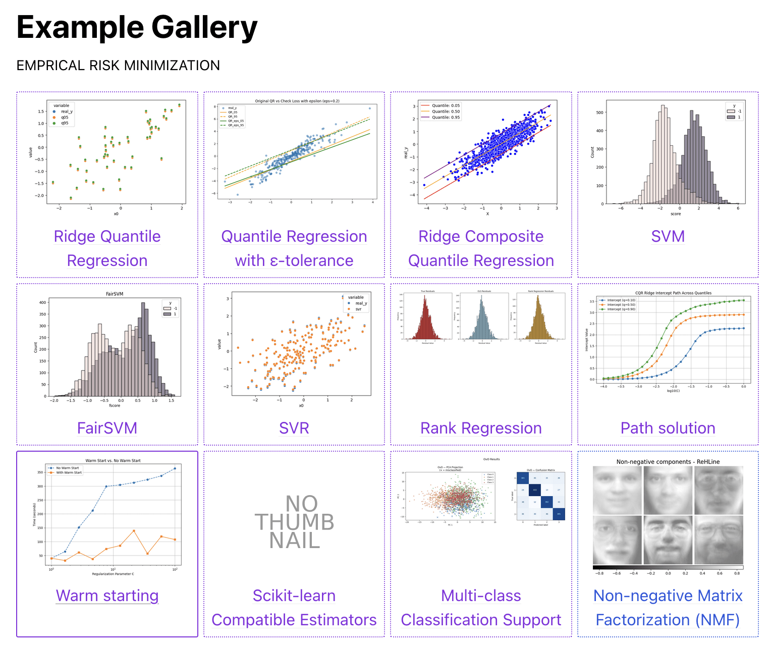
ReHLine Results

A broad range of problems. ReHLine applies to any convex piecewise linear-quadratic loss function (potential for non-smoothness included) with any linear constraints, including the hinge loss, the check loss, the Huber loss, etc.

Super efficient. ReHLine has a linear convergence rate. The per-iteration computational complexity is linear in the sample size.

ReHLine Algo

• Inspired by CD and Liblinear

The linear relationship between primal and dual variables greatly simplifies the computation of CD.

ReHLine Algo

ReHLine Algo

ReHLine Algo

Software. generic/ specialized software

• cvx/cvxpy
• mosek (IPM)
• ecos (IPM)
• scs (ADMM)
• dccp (DCP)
• liblinear -> SVM
• hqreg -> Huber
• lightning -> sSVM

Experiments

• 1000x speed-up for generic solvers
• no worse than specialized solvers

ReHLine SVM

LIBLINEAR

ReHLine

ReHLine QR

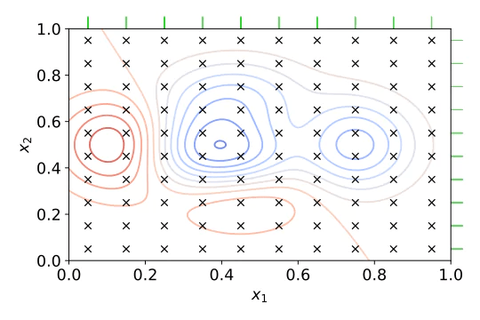
We illustrate our algo in QR using the simulated example from Generate the “Friedman #1” regression problem:

ReHLine QR

We illustrate our algo in QR using the simulated example from Generate the “Friedman #1” regression problem:

1M-Scale Quantile Reg

in 0.5 Second with ReHLine

ReHLine Path Solution

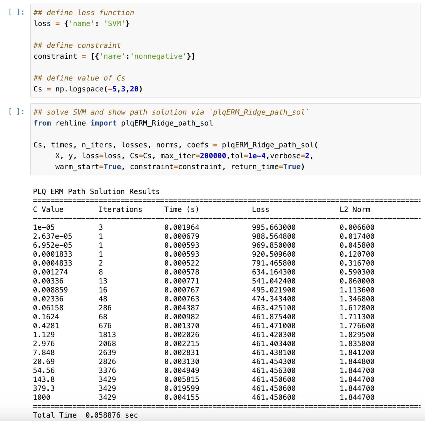
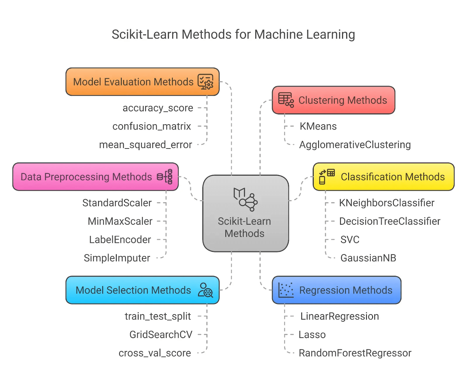
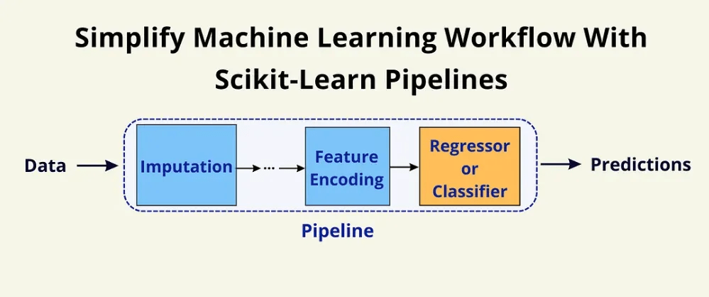
ReHLine integrates with the scikit-learn ecosystem

Source:

- https://medium.com/@sahin.samia/scikit-learn-pipelines-explained-streamline-and-optimize-your-machine-learning-processes-f17b1beb86a4

- https://www.analyticsvidhya.com/blog/2021/06/tune-hyperparameters-with-gridsearchcv/

- https://www.mygreatlearning.com/blog/scikit-machine-learning/

plq_Ridge_Classifier

plq_ElasticNet_Classifier

plq_Ridge_Regressor

plq_ElasticNet_Regressor

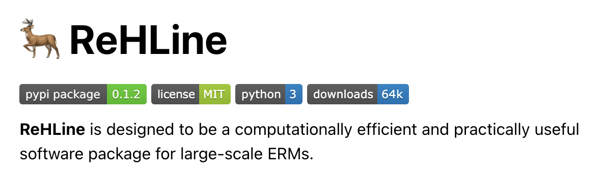
Over the past two years, we have released 8 versions 

399 commits

and achieved ~69K downloads

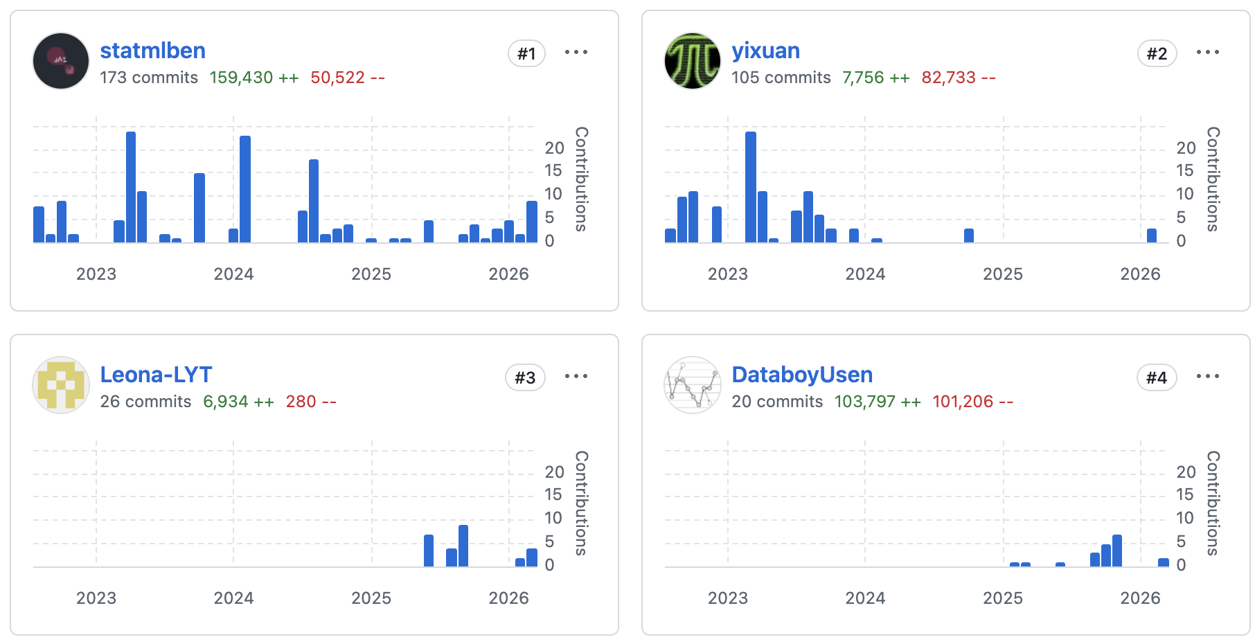
Youtong Li (CUHK)

sklearn compatible interface wrapper

Xiaochen Su (CUHK)

ElasticNet C++ specialized implementation

• Powerful Algo
  • We have improved the computing power of a large category of Regularized Empirical Risk Minimization to the level of LibLinear (linear convergence + linear computation)
• Powerful software
  • Efficient software and C++ implementation. ReHLine is equivalent to LIBLINEAR within SVM.
  • It provides for flexible application concerning losses and constraints through Python/R API, which are intended to tackle a vast array of ML and STAT problems. (e.g. FairSVM).

Summary

Thank you!

If you like ReHLine  please star 🌟 our Github repository, thank you!