RankSEG: A Consistent Framework
for Segmentation
Ben Dai
The Chinese University of Hong Kong


Evolution of Consistency
A statistic is said to be a consistent estimate of any parameter, if when calculated from an indefinitely large sample it tends to be accurately equal to that parameter.
- Fisher (1925) Theory of Statistical Estimation

Ronald Fisher (1890 - 1962)
Evolution of Consistency
Ronald Fisher (1890 - 1962)
A statistic is said to be a consistent estimate of any parameter, if when calculated from an indefinitely large sample it tends to be accurately equal to that parameter.
- Fisher (1925) Theory of Statistical Estimation
\( \hat{\theta}(X_1, \cdots, X_n) \xrightarrow{\mathbb{P}} \theta_0, \quad n \to \infty \)
Probability Consistency
Evolution of Consistency
Fisher, R. A. (1922). On the mathematical foundations of theoretical statistics.

Consistency -- A statistic satisfies the criterion of consistency, if, when it is calculated from the whole population, it is equal to the required parameter.
- Fisher (1922)
Ronald Fisher (1890 - 1962)
Evolution of Consistency
\( \hat{\theta}(X_1, \cdots, X_n) \xrightarrow{\mathbb{P}} \theta_0, \quad n \to \infty \)
Probability Consistency (PC)
\( \hat{\theta} = \hat{\theta}(X_1, \cdots, X_n) \)
Evolution of Consistency
\( \hat{\theta}(X_1, \cdots, X_n) \xrightarrow{\mathbb{P}} \theta_0, \quad n \to \infty \)
Probability Consistency (PC)
\( \hat{\theta} = \hat{\theta}(X_1, \cdots, X_n) \)
Consistency -- A statistic satisfies the criterion of consistency, if, when it is calculated from the whole population, it is equal to the required parameter.
- Fisher (1922)
Evolution of Consistency
Fisher / Fisherian
\( \hat{\theta}(X_1, \cdots, X_n) \xrightarrow{\mathbb{P}} \theta_0, \quad n \to \infty \)
Probability Consistency (PC)
\( \hat{\theta} = \hat{\theta}(X_1, \cdots, X_n) \)
\( \hat{\theta}= \hat{\theta}(F_n) \)
Fisher / Fisherian

Evolution of Consistency
Fisher / Fisherian
\( \hat{\theta}(F_n) \xrightarrow{\mathbb{P}} \theta(F), \quad n \to \infty \)
\( \hat{\theta}(X_1, \cdots, X_n) \xrightarrow{\mathbb{P}} \theta_0, \quad n \to \infty \)
Probability Consistency (PC)
\( \hat{\theta} = \hat{\theta}(X_1, \cdots, X_n) \)
\( \hat{\theta}= \hat{\theta}(F_n) \)
\(\theta(F) = \theta_0\)
Fisher / Fisherian
(when it is calculated from the whole population)
Evolution of Consistency
Fisher / Fisherian
\( \hat{\theta}(F_n) \xrightarrow{\mathbb{P}} \theta(F), \quad n \to \infty \)
\( \hat{\theta}(X_1, \cdots, X_n) \xrightarrow{\mathbb{P}} \theta_0, \quad n \to \infty \)
Probability Consistency (PC)
\( \hat{\theta} = \hat{\theta}(X_1, \cdots, X_n) \)
\( \hat{\theta}= \hat{\theta}(F_n) \)
\(\theta(F) = \theta_0\)
Fisher Consistency (FC)
Fisher / Fisherian
Evolution of Consistency
Fisher / Fisherian
\( \hat{\theta}(F_n) \xrightarrow{\mathbb{P}} \theta(F), \quad n \to \infty \)
\( \hat{\theta}(X_1, \cdots, X_n) \xrightarrow{\mathbb{P}} \theta_0, \quad n \to \infty \)
Probability Consistency (PC)
\( \hat{\theta} = \hat{\theta}(X_1, \cdots, X_n) \)
\( \hat{\theta}= \hat{\theta}(F_n) \)
\(\theta(F) = \theta_0\)
Fisher Consistency (FC)
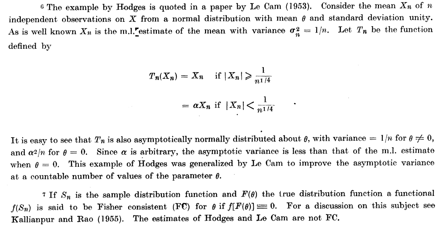
Gerow, K. (1989): In fact, for many years, Fisher took his two definitions to be describing the same thing... Fisher 34 years to polish the definitions of consistency to their present form [from FC to PC].
Evolution of Consistency
Evolution of Consistency
CR, Rao. (1962) Apparent Anomalies and Irregularities in Maximum Likelihood Estimation
Evolution of Consistency
Fisher / Fisherian
\( \hat{\theta}(F_n) \xrightarrow{\mathbb{P}} \theta(F), \quad n \to \infty \)
\( \hat{\theta}(X_1, \cdots, X_n) \xrightarrow{\mathbb{P}} \theta_0, \quad n \to \infty \)
Probability Consistency (PC)
\( \hat{\theta} = \hat{\theta}(X_1, \cdots, X_n) \)
\( \hat{\theta}= \hat{\theta}(F_n) \)
\(\theta(F) = \theta_0\)
Fisher / Fisherian
(when it is calculated from the whole population)
Fisher Consistency (FC)
Evolution of Consistency
Fisher / Fisherian
\( \hat{\theta}(F_n) \xrightarrow{\mathbb{P}} \theta(F), \quad n \to \infty \)
\( \hat{\theta}(X_1, \cdots, X_n) \xrightarrow{\mathbb{P}} \theta_0, \quad n \to \infty \)
Probability Consistency (PC)
\( \hat{\theta} = \hat{\theta}(X_1, \cdots, X_n) \)
\( \hat{\theta}= \hat{\theta}(F_n) \)
\(\theta(F) = \theta_0\)
Glivenko–Cantelli theorem (1933);
Fisher Consistency (FC)
Fisher / Fisherian
Fisher assumed:
Evolution of Consistency: PC and FC

CR, Rao. (1962) Apparent Anomalies and Irregularities in Maximum Likelihood Estimation
With continuous functionals; FC iff PC.
FC
-
Strength
-
FC almost implies PC (with continuous functionals)
- Distribution-free
- Practical and fundamentally true
-
FC provides a deterministic equality
- Easy to use
- Directly motivate a consistent method via the FC equality
-
FC almost implies PC (with continuous functionals)
FC
-
Strength
-
FC almost implies PC (with continuous functionals)
- Distribution-free
- Practical and fundamentally true
-
FC provides a deterministic equality
- Easy to use
- Directly motivate a consistent method via the FC equality
-
FC almost implies PC (with continuous functionals)
-
Weakness
-
Not all estimators can be easily expressed in the form of an empirical cdf.
-
- MLE / ERM are functionals of an empirical cdf
- FC has become the minimal requirement for ML methods
- You are estimating what you want
FC in ML
Classification
- Data: \( \mathbf{X} \in \mathbb{R}^d \to Y \in \{0,1\} \)
- Decision function: \( \delta(\mathbf{X}): \mathbb{R}^d \to \{0,1\} \)
- Evaluation:
$$ Acc( \delta) = \mathbb{E}\big( \mathbb{I}( Y = \delta(\mathbf{X}) )\big) $$
FC in ML
Classification
- Data: \( \mathbf{X} \in \mathbb{R}^d \to Y \in \{0,1\} \)
- Decision function: \( \delta(\mathbf{X}): \mathbb{R}^d \to \{0,1\} \)
- Evaluation:
$$ Acc( \delta) = \mathbb{E}\big( \mathbb{I}( Y = \delta(\mathbf{X}) )\big) $$
ML Consistency. if when calculated from an indefinitely large sample its performance tends to be accurately equal to that parameter the best evaluation performance.
FC in ML
How can we develop an FC method?
Classification
- Data: \( \mathbf{X} \in \mathbb{R}^d \to Y \in \{0,1\} \)
- Decision function: \( \delta(\mathbf{X}): \mathbb{R}^d \to \{0,1\} \)
- Evaluation:
$$ Acc( \delta) = \mathbb{E}\big( \mathbb{I}( Y = \delta(\mathbf{X}) )\big) $$
(Plug-in rule).
$$ \delta^* = \argmax_{\delta} \ Acc(\delta) $$
$$ \delta^* = \delta^*(F) \to \delta^*(F_n)$$
ML Consistency. if when calculated from an indefinitely large sample its performance tends to be accurately equal to that parameter the best evaluation performance.
$$ \delta^* = \argmax_{\delta} \ Acc(\delta) \ \ \to \ \delta^*(\mathbf{x}) = \mathbb{I}( p(\mathbf{x}) \geq 0.5 ) $$
$$ p(\mathbf{x}) = \mathbb{P}(Y=1|\mathbf{X}=\mathbf{x})$$
- Obtain the probabilistic form of the Bayes rule (optimal decision)
- Re-write the Bayes rule as \( \delta(F) \)
(Plug-in rule).
Simplest FC method
$$\delta^*(F)$$
$$ \delta^* = \argmax_{\delta} \ Acc(\delta) \ \ \to \ \delta^*(\mathbf{x}) = \mathbb{I}( p(\mathbf{x}) \geq 0.5 ) $$
$$ p(\mathbf{x}) = \mathbb{P}(Y=1|\mathbf{X}=\mathbf{x})$$
- Replace \(F\) by \(F_n\):
$$ \hat{\delta}(\mathbf{x}) = \mathbb{I}( \hat{p}_n(\mathbf{x}) \geq 0.5 ) $$
Plug-in rule method:
- Step 1. Estimate \( \hat{p}_n \) from MLE
- Step 2. Plug-in \( \hat{p}_n \) in \( \hat{\delta}(\mathbf{x}) \)
(Plug-in rule).
Simplest FC method
- Obtain the probabilistic form of the Bayes rule (optimal decision)
- Re-write the Bayes rule as \( \delta(F) \)
Examples
kNN classifier
kernel logistic regression
nonparametric
$$\delta^*(F)$$
FC loss functions
(ERM via a surrogate loss).
- Obtain \( \hat{f} \) from a ERM with a surrogate loss (\( \hat{\delta} = \mathbb{I}(\hat{f} \geq 0) \))
$$ \hat{f}_{\phi} = \argmin_f \mathbb{E}_n \phi\big(Y f(\mathbf{X}) \big) $$
$$ f_\phi = \argmin_f \mathbb{E} \phi\big(Y f(\mathbf{X}) \big)$$
$$Acc \big ( \hat{\delta}(F_n) \big) \xrightarrow{\mathbb{P}} Acc \big( \delta(F) \big) = \max_{\delta} Acc(\delta)$$
FC leads to conditions for "consistent" surrogate losses
Theorem. (Bartlett et al. (2006); informal) Let \(\phi\) be convex. \(\phi\) is "consistent" iff it is differentiable at 0 and \( \phi'(0) < 0 \).
Convex loss. Lin (2004), Zhang (2004), Lugosi and Vayatis (2004), Steinwart (2005), Bartlett et al. (2006)
(Plug-in rule).
Simplest FC method
- Obtain the probabilistic form of the Bayes rule (optimal decision)
- Re-write the Bayes rule as \( \delta(F) \)
- Replace \(F\) by \(F_n\), to obtain a FC method
- Evaluation:
$$ Acc( \delta) = \mathbb{E}\big( \mathbf{1}( Y = \delta(\mathbf{X}) )\big) $$
- Optimal Rule:
$$ \delta^* = \argmax_{\delta} \ F1(\delta) \ \ \to \ \delta^*(\mathbf{x}) = \mathbf{1}( p(\mathbf{x}) \geq p_0 ) $$
$$F1(\delta)$$
where \(p_0 = F1^* / 2 \leq 0.5 \), it is also truncation, but not at 0.5!
Evaluation really matters!
Medical image segmentation
In the medical domain, over 70% of prize-money Kaggle competitions are segmentation
Autonomous vehicles
The "Cityscapes" Benchmark Dominance

Agriculture
John Deere claims "segmentation" allows farmers to reduce herbicide use by up to 77%


Segmentation


Input
output
Input: \(\mathbf{X} \in \mathbb{R}^d\)
Outcome: \(\mathbf{Y} \in \{0,1\}^d\)
Segmentation function:
- \( \pmb{\delta}: \mathbb{R}^d \to \{0,1\}^d\)
- \( \pmb{\delta}(\mathbf{X}) = ( \delta_1(\mathbf{X}), \cdots, \delta_d(\mathbf{X}) )^\intercal \)
Predicted segmentation set:
- \( I(\pmb{\delta}(\mathbf{X})) = \{j: \delta_j(\mathbf{X}) = 1 \}\)
Segmentation
Input
output
$$ Y_j | \mathbf{X}=\mathbf{x} \sim \text{Bern}\big(p_j(\mathbf{x})\big)$$
$$ p_j(\mathbf{x}) := \mathbb{P}(Y_j = 1 | \mathbf{X} = \mathbf{x})$$
Probabilistic model:
The Dice and IoU metrics are introduced and widely used in practice:


Evaluation
IoU
The Dice and IoU metrics are introduced and widely used in practice:
Evaluation
Goal: learn segmentation function \( \pmb{\delta} \) maximizing Dice / IoU
Dice
- Given training data \( \{\mathbf{x}_i, \mathbf{y}_i\} _{i=1, \cdots, n}\), most existing methods characterize segmentation as a classification problem:

Existing frameworks
- Given training data \( \{\mathbf{x}_i, \mathbf{y}_i\} _{i=1, \cdots, n}\), most existing methods characterize segmentation as a classification problem:
Existing frameworks
Classification-based loss


CE + Focal
CE
CE

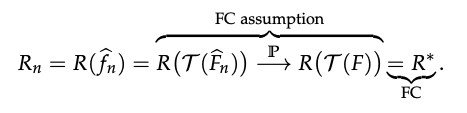
We aim to leverage the principles of FC to develop an consistent segmentation method.
FC in Segmentation
Recall (Plug-in rule in classification).
$$ \delta^* = \argmax_{\delta} \ Acc(\delta) $$
$$ \delta^* = \delta^*(F) \to \delta^*(F_n)$$
We aim to leverage the principles of FC to develop an consistent segmentation method.
FC in Segmentation
Recall (Plug-in rule in segmentation).
$$ \delta^* = \argmax_{\delta} \ Acc(\delta) $$
$$ \delta^* = \delta^*(F) \to \delta^*(F_n)$$
$$ \pmb{\delta}^* = \text{argmax}_{\pmb{\delta}} \ \text{Dice}_\gamma ( \pmb{\delta})$$
Bayes segmentation rule
What form would the Bayes segmentation rule take?
Bayes segmentation rule
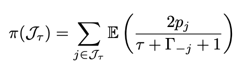
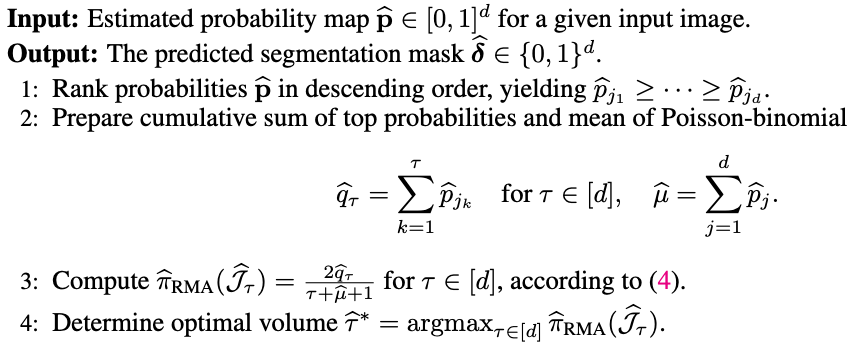
Theorem 1 (Dai and Li, 2023). A segmentation rule \(\pmb{\delta}^*\) is a global maximizer of \(\text{Dice}_\gamma(\pmb{\delta})\) if and only if it satisfies that

\( \tau^*(\mathbf{x}) \) is called optimal segmentation volume, defined as

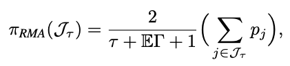
$$ \tau^* = \arg\max_{\tau \in \{0,1,\cdots,d\}} \Big( \sum_{j \in J_\tau(\mathbf{x})} \mathbb{E} \big( \frac{2p_j(\mathbf{x})}{\tau + \Gamma_{-j}(\mathbf{x}) + \gamma + 1 } \big) + \gamma \mathbb{E} \big( \frac{1}{\tau + \Gamma + \gamma} \big) \Big) $$
The Dice measure is separable w.r.t. \(j\)

Bayes segmentation rule


Bayes segmentation rule

Bayes segmentation rule
Bayes segmentation rule
Theorem 1 (Dai and Li, 2023). A segmentation rule \(\pmb{\delta}^*\) is a global maximizer of \(\text{Dice}_\gamma(\pmb{\delta})\) if and only if it satisfies that
\( \tau^*(\mathbf{x}) \) is called optimal segmentation volume, defined as
$$ \tau^* = \arg\max_{\tau \in \{0,1,\cdots,d\}} \Big( \sum_{j \in J_\tau(\mathbf{x})} \mathbb{E} \big( \frac{2p_j(\mathbf{x})}{\tau + \Gamma_{-j}(\mathbf{x}) + \gamma + 1 } \big) + \gamma \mathbb{E} \big( \frac{1}{\tau + \Gamma + \gamma} \big) \Big) $$
Theorem 1 (Dai and Li, 2023). A segmentation rule \(\pmb{\delta}^*\) is a global maximizer of \(\text{Dice}_\gamma(\pmb{\delta})\) if and only if it satisfies that
\( \tau^*(\mathbf{x}) \) is called optimal segmentation volume, defined as
Obs: both the Bayes segmentation rule \(\pmb{\delta}^*(\mathbf{x})\) and the optimal volume function \(\tau^*(\mathbf{x})\) are achievable when the conditional probability \(\mathbf{p}(\mathbf{x}) = ( p_1(\mathbf{x}), \cdots, p_d(\mathbf{x}) )^\intercal\) is well-estimated
Bayes segmentation rule
$$ \tau^* = \arg\max_{\tau \in \{0,1,\cdots,d\}} \Big( \sum_{j \in J_\tau(\mathbf{x})} \mathbb{E} \big( \frac{2p_j(\mathbf{x})}{\tau + \Gamma_{-j}(\mathbf{x}) + \gamma + 1 } \big) + \gamma \mathbb{E} \big( \frac{1}{\tau + \Gamma + \gamma} \big) \Big) $$
Theorem 1 (Dai and Li, 2023). A segmentation rule \(\pmb{\delta}^*\) is a global maximizer of \(\text{Dice}_\gamma(\pmb{\delta})\) if and only if it satisfies that
\( \tau^*(\mathbf{x}) \) is called optimal segmentation volume, defined as
where \(J_\tau(\mathbf{x})\) is the index set of the \(\tau\)-largest probabilities, \(\Gamma(\mathbf{x}) = \sum_{j=1}^d {B}_{j}(\mathbf{x})\), and \( {\Gamma}_{- j}(\mathbf{x}) = \sum_{j' \neq j} {B}_{j'}(\mathbf{x})\) are Poisson-binomial random variables.
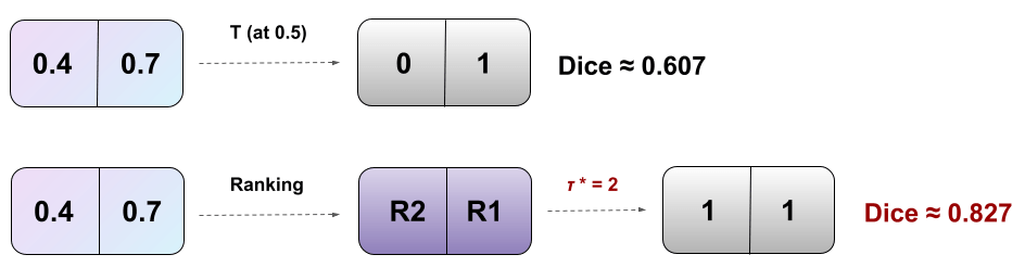
RankDice inspired by Thm 1 (plug-in rule)
-
Ranking the conditional probability \(p_j(\mathbf{x})\)
Plug-in rule
Theorem 1 (Dai and Li, 2023+). A segmentation rule \(\pmb{\delta}^*\) is a global maximizer of \(\text{Dice}_\gamma(\pmb{\delta})\) if and only if it satisfies that
\( \tau^*(\mathbf{x}) \) is called optimal segmentation volume, defined as
RankDice inspired by Thm 1
-
Ranking the conditional probability \(p_j(\mathbf{x})\)
-
searching for the optimal volume of the segmented features \(\tau(\mathbf{x})\)
Plug-in rule
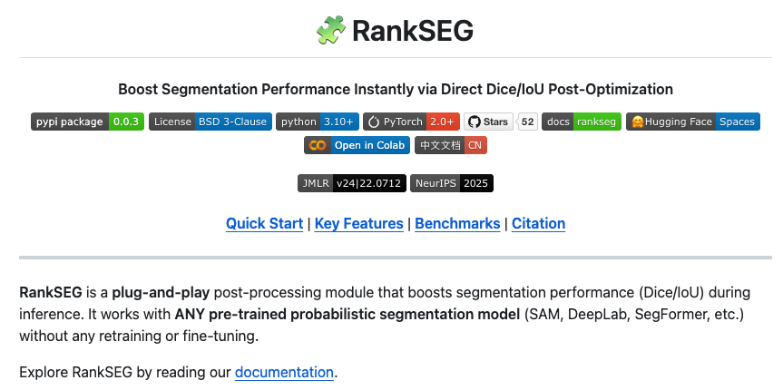
RankSEG
RankSEG


RankSEG
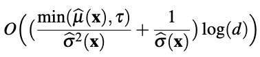
O( d log(d) )
RankSEG
O( d^2 )
RankSEG
$$ \tau^* = \arg\max_{\tau \in \{0,1,\cdots,d\}} \Big( \sum_{j \in J_\tau(\mathbf{x})} \mathbb{E} \big( \frac{2p_j(\mathbf{x})}{\tau + \Gamma_{-j}(\mathbf{x}) + \gamma + 1 } \big) + \gamma \mathbb{E} \big( \frac{1}{\tau + \Gamma + \gamma} \big) \Big) $$
Blind approximation (BA; Dai and Li 2023). In high-D segmentation, the difference in distributions between \(\Gamma(\mathbf{x})\) and \(\Gamma_{-j}(\mathbf{x})\) is negligible.
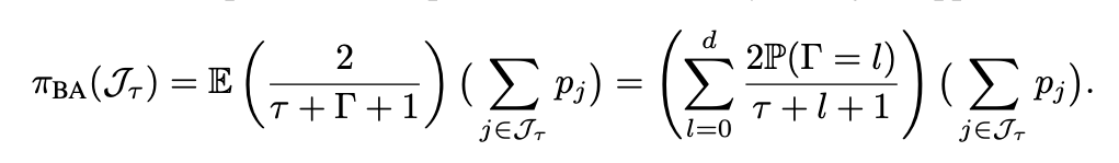
$$ \approx $$
$$\to 0 (d \to \infty)$$
Lemma 5 in Dai and Li (2023)
RankSEG: BA Algo
Blind approximation (BA; Dai and Li 2023). In high-D segmentation, the difference in distributions between \(\Gamma(\mathbf{x})\) and \(\Gamma_{-j}(\mathbf{x})\) is negligible.
$$ \approx $$
$$\to 0 (d \to \infty)$$
Lemma 5 in Dai and Li (2023)
$$ \tau^* = \arg\max_{\tau \in \{0,1,\cdots,d\}} \Big( \sum_{j \in J_\tau(\mathbf{x})} \mathbb{E} \big( \frac{2p_j(\mathbf{x})}{\tau + \Gamma_{-j}(\mathbf{x}) + \gamma + 1 } \big) + \gamma \mathbb{E} \big( \frac{1}{\tau + \Gamma + \gamma} \big) \Big) $$
RankSEG: BA Algo

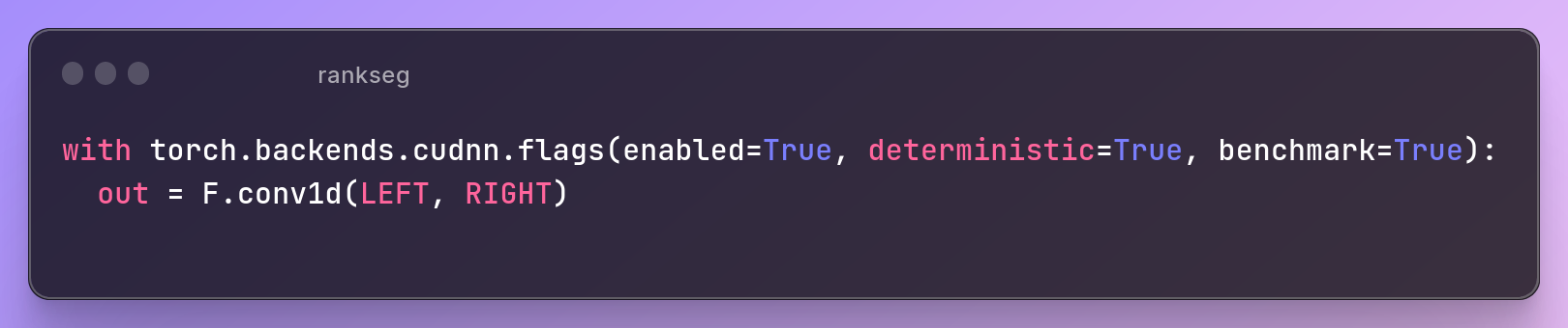
GPU via CUDA
O( d log(d) ) 😄
(approx 100 times slower than T (at 0.5) 🥲)
RankSEG: BA Algo
RankSEG: RMA
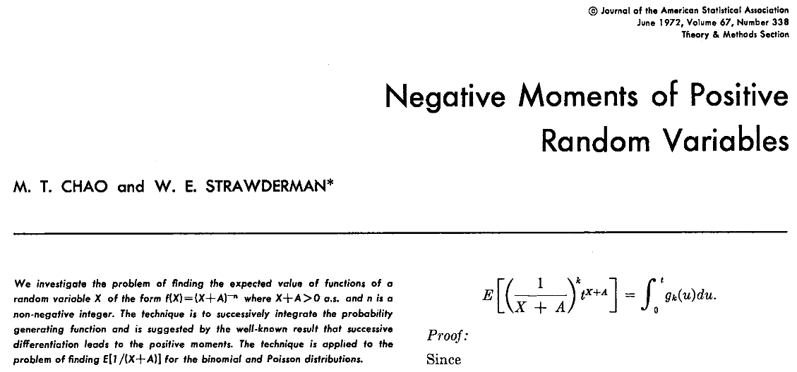
Chao, M. T., & Strawderman, W. E. (1972). JASA
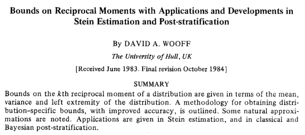
Wooff, David A. (1985) JRSS-b
RankSEG: RMA
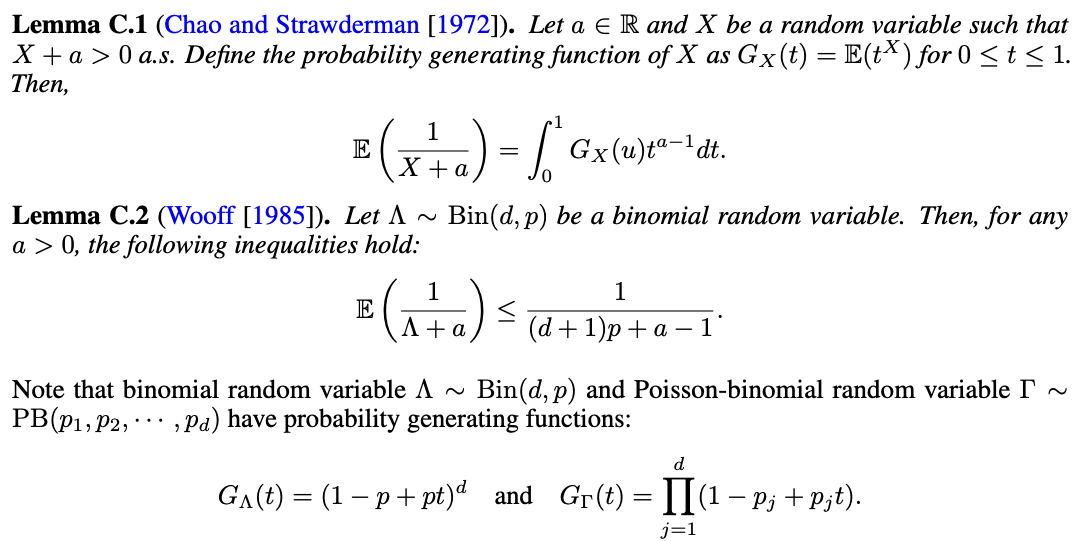
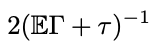
Theorem 2 (Wang and Dai, 2025). (Reciprocal moment approximation to RankSEG). Let \(\Gamma\) be a Poisson-binomial r.v., then for any \(\tau \geq 1\),
$$ (\mathbb{E}\Gamma + \tau)^{-1} \leq \mathbb{E}(\Gamma + \tau)^{-1} \leq \left(\frac{d+1}{d}\mathbb{E}\Gamma + \tau - 1\right)^{-1}. $$

Zixun Wang (CUHK)
$$ \approx $$
$$ \approx $$
$$\to 0 (d \to \infty)$$
Theorem 2 in Wang and Dai (2025)
RankSEG: RMA
$$ \approx $$
$$ \approx $$
$$\to 0 (d \to \infty)$$
Theorem 2 in Wang and Dai (2025)
RankSEG: RMA
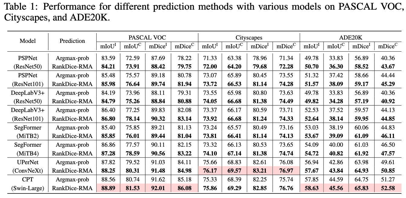
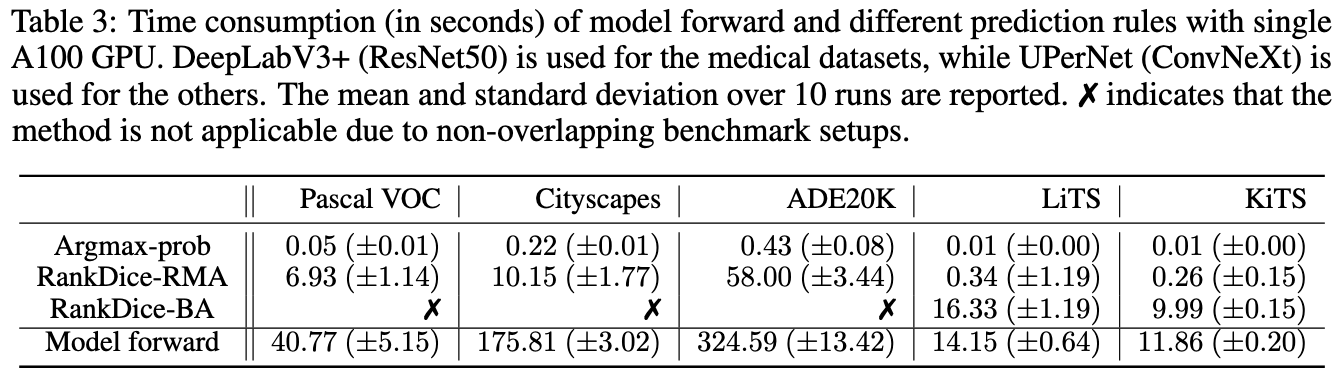
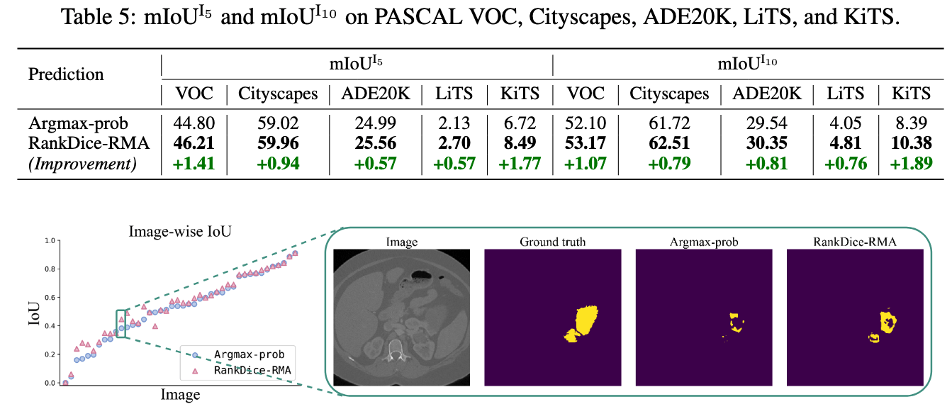
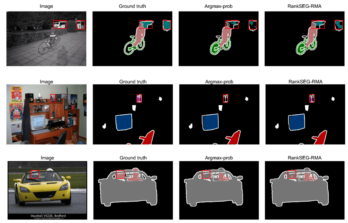
- Three segmentation benchmark: VOC, CityScapes, ADE20K
RankSEG: Experiments

Source: Visual Object Classes Challenge 2012 (VOC2012)
- Three segmentation benchmark: VOC, CityScapes, ADE20K
RankSEG: Experiments
Source: Visual Object Classes Challenge 2012 (VOC2012)

Source: The Cityscapes Dataset: Semantic Understanding of Urban Street Scenes
- Three segmentation benchmark: VOC, CityScapes, ADE20K
RankSEG: Experiments
Source: Visual Object Classes Challenge 2012 (VOC2012)
Source: The Cityscapes Dataset: Semantic Understanding of Urban Street Scenes
Zhou, Bolei, et al. "Semantic understanding of scenes through the ade20k dataset." IJCV
- Three segmentation benchmark: VOC, CityScapes, ADE20K
RankSEG: Experiments
-
Three segmentation benchmarks: VOC, CityScapes, ADE20K
- Standard benchmarks, NOT cherry-picks
- Commonly used models: DeepLab-V3+, PSPNet, SegFormer
- The proposed framework VS. the existing frameworks
- Based on the SAME trained neural networks
- No implementation tricks
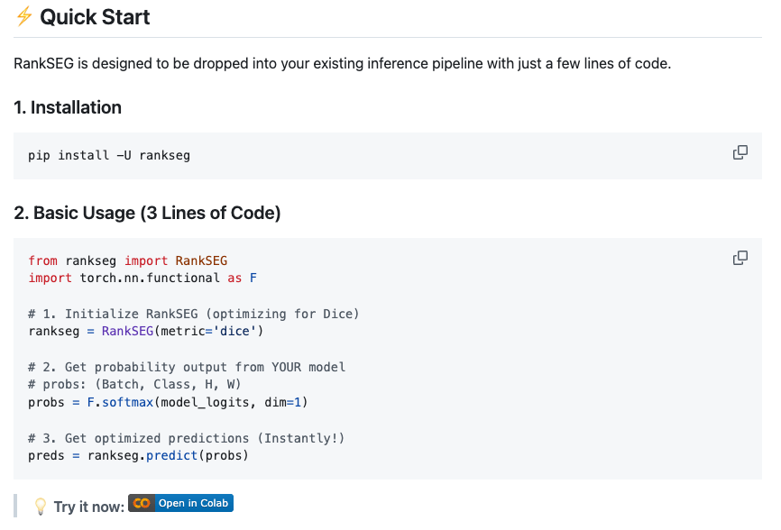
- Open-Source python module and codes for replication
- All trained neural networks available for download
RankSEG: Experiments
RankSEG: Experiments
RankSEG: Experiments

RankSEG: Experiments

RankSEG: Experiments
RankSEG: Experiments
More experimental results in Dai and Li (2023) and Wang and Dai (2025)
RankSEG: Experiments

Fisher consistency or Classification-Calibration
(Lin, 2004, Zhang, 2004, Bartlett et al 2006)
Classification
Segmentation
RankSEG: Theory

RankSEG: Theory

RankSEG: Theory

RankSEG: Theory

RankSEG: Theory
- mRankDice: extension and challenge
- RankIoU
- Simulation
- Probability calibration
- ....
More results
-
To our best knowledge, the proposed ranking-based segmentation framework RankSEG, is a consistent segmentation framework with respect to the Dice/IoU metric.
-
BA and RMA algorithms with GPU parallel execution and are developed to implement the proposed framework in large-scale and high-dimensional segmentation.
-
We establish a theoretical foundation of segmentation with respect to the Dice metric, such as the Bayes rule, Dice-calibration, and a convergence rate of the excess risk for the proposed RankDice framework, and indicate inconsistent results for the existing methods.
-
Our experiments suggest that the improvement of RankSEG over the existing frameworks is significant.
Contribution
Thank you!

If you like RankSEG please star 🌟 our Github repository, thank you for your support!

- Dai, B., & Li, C. (2023). RankSEG: A Consistent Ranking-based Framework for Segmentation. Journal of Machine Learning Research.
- Wang, Z., & Dai, B. (2025). RankSEG-RMA: An Efficient Segmentation Algorithm via Reciprocal Moment Approximation. NeurIPS.