Landmark shape spaces with induced metrics
Stefan Sommer, University of Copenhagen

Faculty of Science, University of Copenhagen
Aarhus University, September 2026
From landmark configurations to shapes
Two approaches:
- Kendall's shape space: Euclidean metric, \(\mathrm{SE}(d)\) quotient, size normalization
- Procrustes pre-alignment + metric induced by right-inviant metric on \(\mathrm{Diff}(\mathrm R^d)\)
Goal: motivation and unification
\(\mathrm{Land}^n(\mathbb R^d)=\{(q_1,\ldots,q_n)|q_i\not=q_j\mathrm{\ for\ }i\not=j\}\)

Shape stochastics, conditional processes, scores and inference
w/ Peter W. Michor, Sarang Joshi, Frank v.d. Meulen, Erlend Grong, Rasmus Nielsen, Christy Hipsley, Sofia Stoustrup, Libby Baker, Gefan Yang, Michael Severinsen, Jingchao Zhou
Villum foundation
Novo nordisk foundation
University of Copenhagen
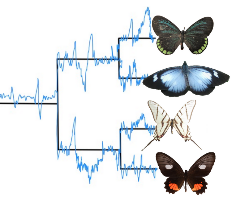

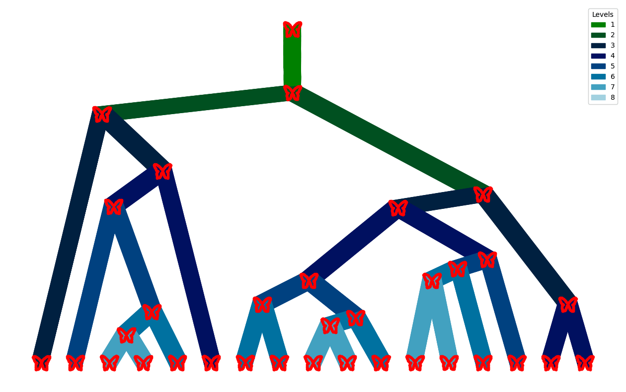
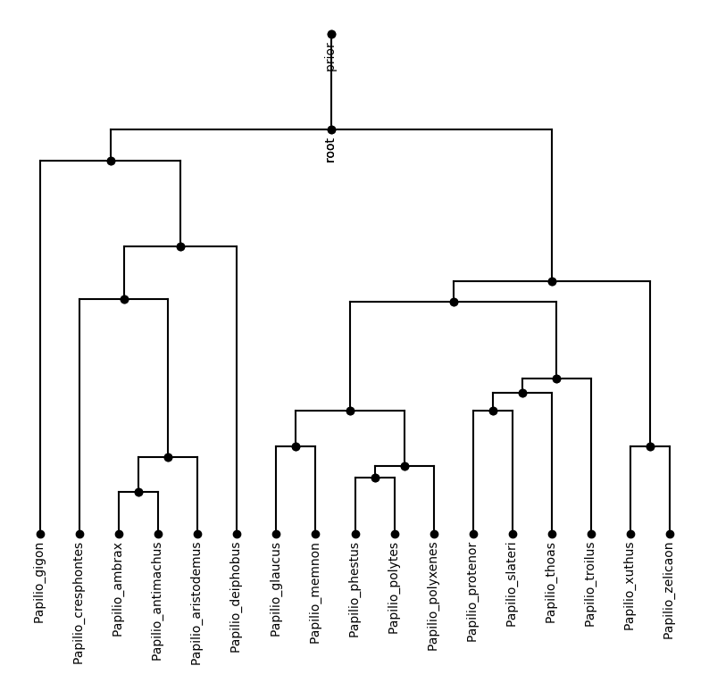
Brownian motion model of trait evolution
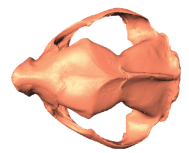
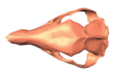
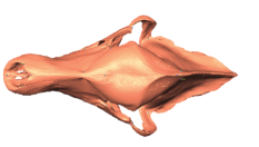
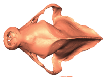
Brown. motion
Brown. motion
Brown. motion
Brown. motion
branch (independent children)
incorporate leaf observations \(x_{V_T}\) into probabilistic model:
\(p(X_t|x_{V_T})\)
Felsenstein's pruning algorithm for shapes
Brown. motion
Brown. motion
Brown. motion
Brown. motion
1) define shape Brownian motion
2) incorporate shape observations in the nonlinear process
3) perform inference in the full model
Stochastics of shapes
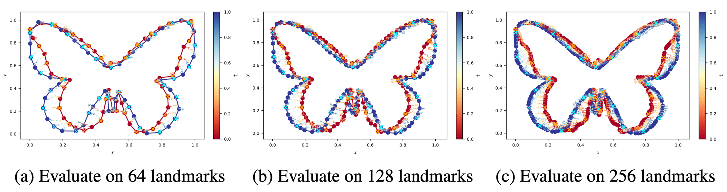
Stochastic processes that
- apply to landmarks, curves, surfaces and images
- are independent of discretization
- preserve shape structure
- equivariant to acting groups
- can be recovered from discretizations
\(\Large\Rightarrow\) - model correlations between points
- are nonlinear
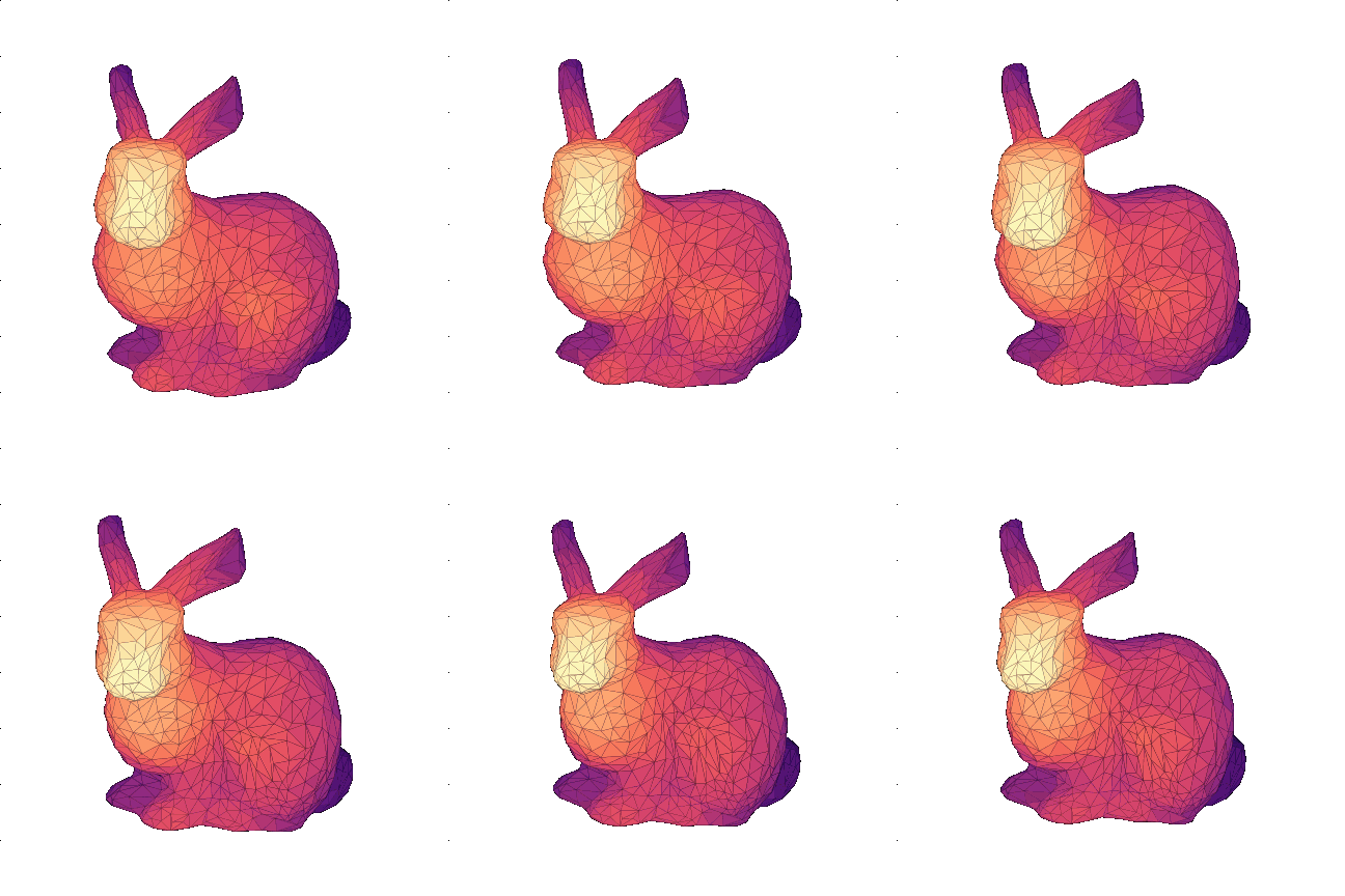
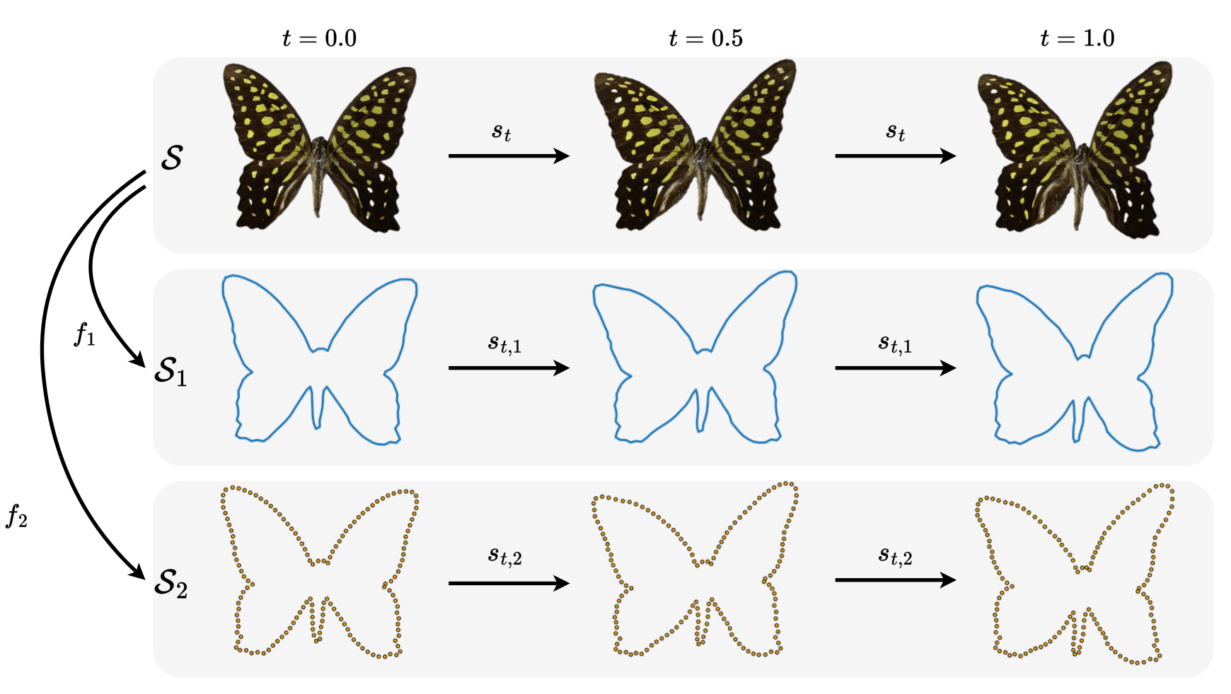
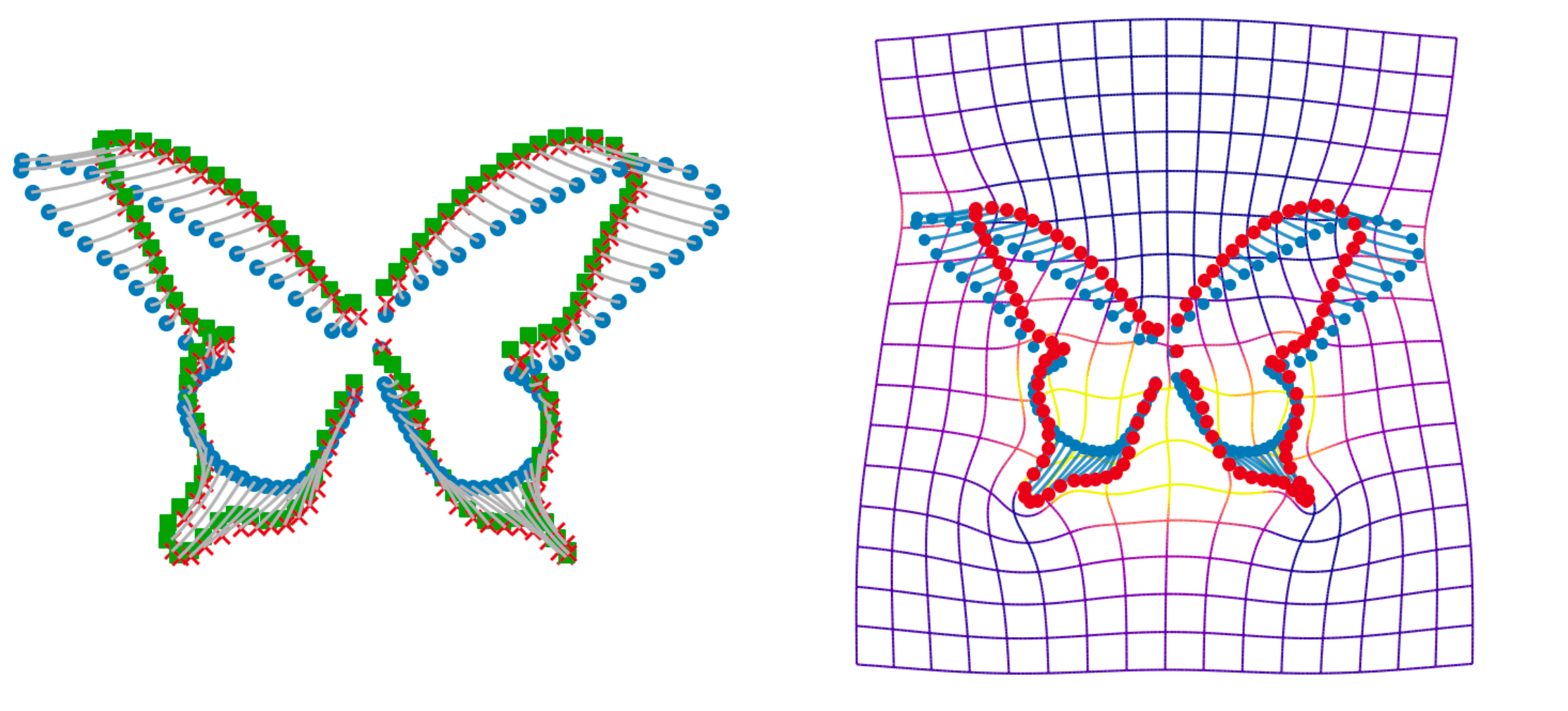
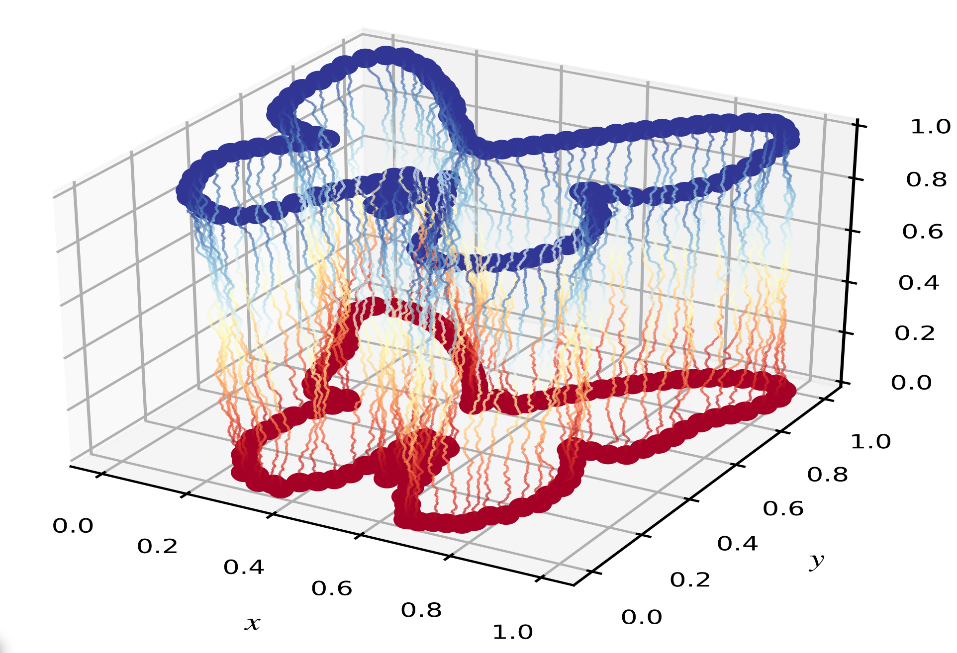
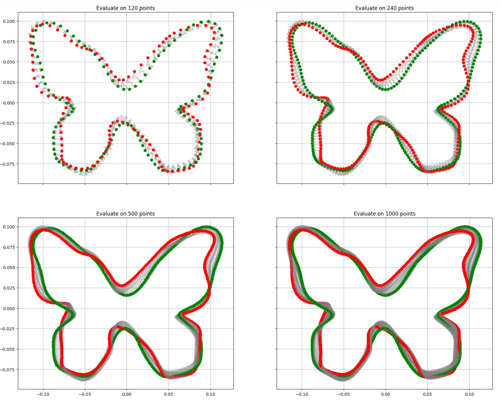
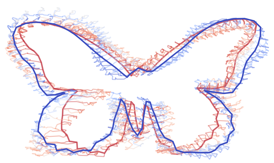
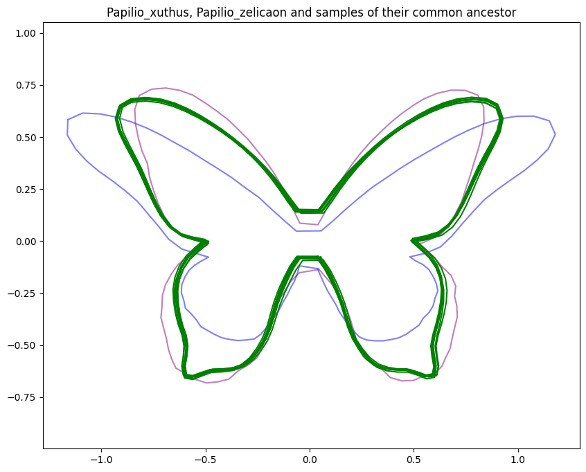
Kunita flows: evolving butterfly
Shapes, deformations and nonlinearity
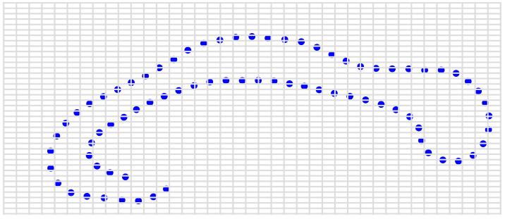
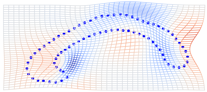
action:
\(\phi.s=\phi\circ s\) (shapes)
\(\phi.s=s\circ\phi^{-1}\) (images)
\( \phi \)
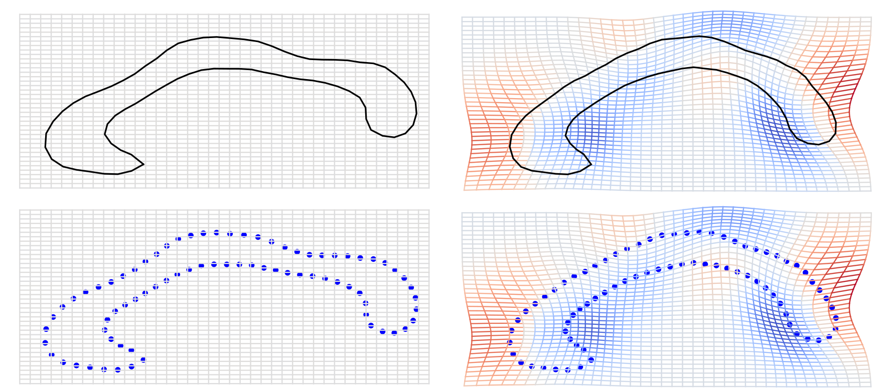
\( \phi \) warp of domain \(\Omega\) (2D or 3D space)
landmarks: \(s=(x_1,\ldots,x_n)\)
curves: \(s: \mathbb S^1\to\mathbb R^2\)
surfaces: \(s: \mathbb S^2\to\mathbb R^3\)
Geometric + metric view
\( \phi_t:[0,T]\to G\subset\mathrm{Diff}(\Omega) \), \(\frac{d}{dt}\phi_t=v\circ\phi_t^{-1}\)
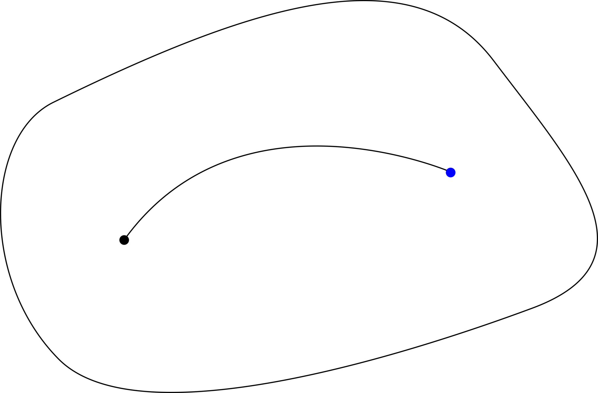
LDDMM: Grenander, Miller, Trouve, Younes, Christensen, Joshi, et al.
Evolution with noise
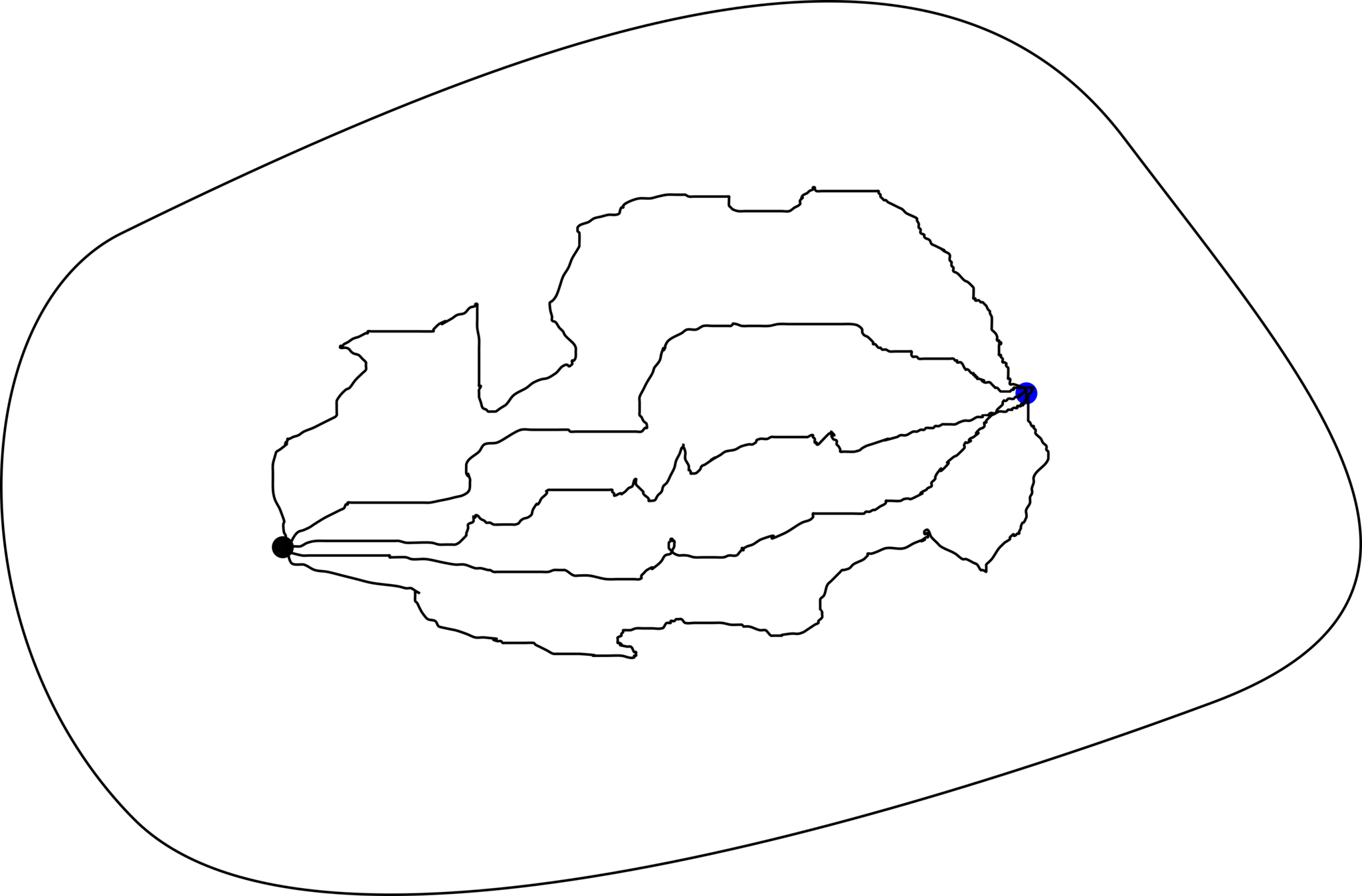
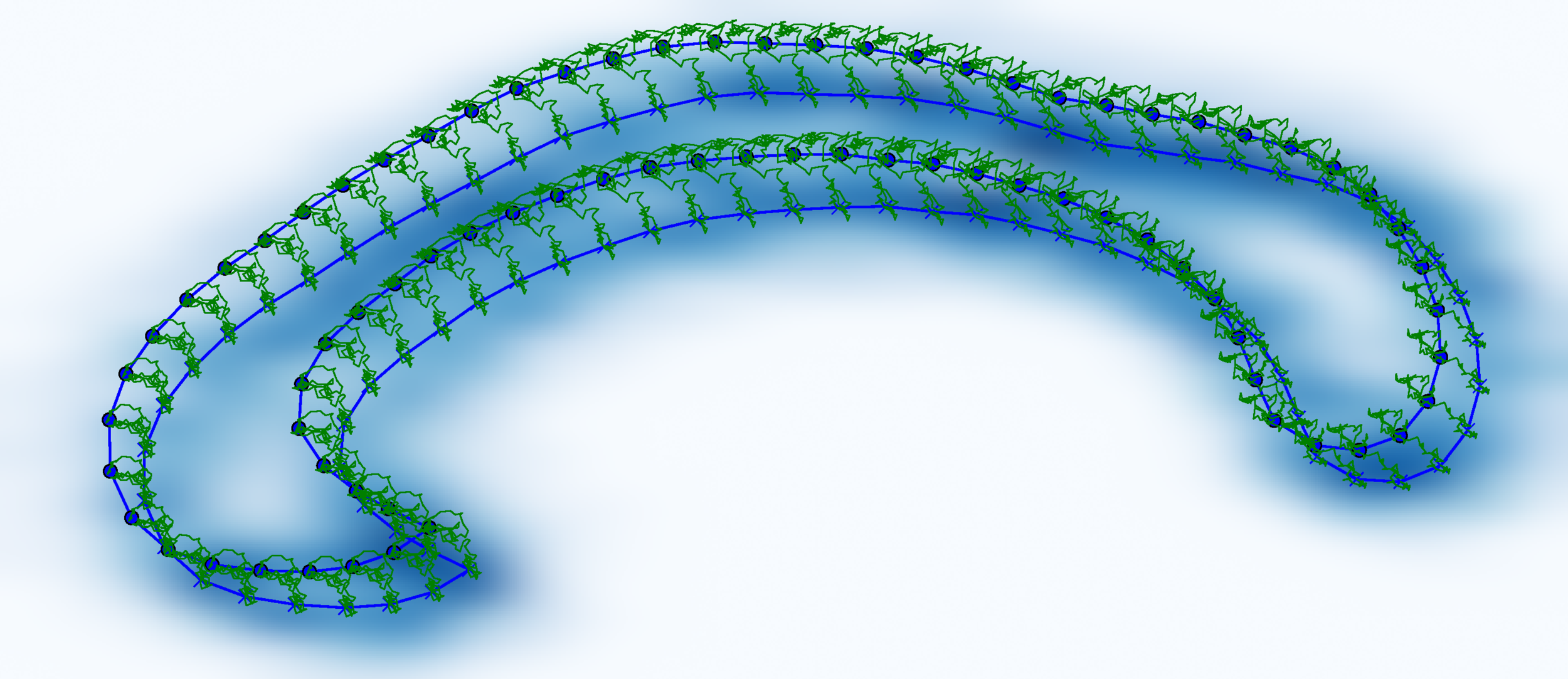
Markussen,CVIU'07; Budhiraja,Dupuis,Maroulas,Bernoulli'10
Trouve,Vialard,QAM'12;Vialard,SPA'13;Marsland/Shardlow,SIIMS'17
Arnaudon,Holm,Sommer,IPMI'17; FoCM'18; JMIV'19
Arnaudon,v.d. Meulen,Schauer,Sommer'21
geodesic ODE
perturbed SDE
Kunita flows
\(\phi_{s,t}:\mathbb{R}^d \times \Omega \to \mathbb{R}^d\), \(0 \le s \le t\) indexed family of random fields s.t. for each \(s,t,\omega\), the map \(\phi_{s,t}(\cdot,\omega):\mathbb{R}^d \to \mathbb{R}^d\) is measurable.
The family is called a stochastic flow if
1. \(s,t,x \mapsto \phi_{s,t}(x)\) is continuous in \(s,t,x\) in probability,
2. \(\phi_{s,s} = \mathrm{Id}_{\mathbb{R}^d}\) for all \(s\),
3. \(\phi_{s,t} \circ \phi_{t,u} = \phi_{s,u}\) for all \(s \le t \le u\).
If increments \(\phi_{t_i,t_{i+1}}\) are independent for any \(0 \le t_0 \le t_1 \le \cdots \le t_n\) and \(\phi_{s,t}(x)\) is continuous in \(t\) a.s., then \(\phi_{s,t}\) is called a Brownian flow.
Local characteristics:
\[b_t(x) = \lim_{h \downarrow 0}\frac{1}{h}\mathbb{E}\big[\phi_{t,t+h}(x)-x\big]\qquad\qquad\qquad\ \]
\[a_t(x,y) = \lim_{h \downarrow 0}\frac{1}{h}\mathbb{E}\Big[(\phi_{t,t+h}(x)-x)(\phi_{t,t+h}(y)-y)^T\Big]\]
Kunita,'86,'97
Flows and stochastic integral
Theorem: With additional assumptions, there exists a a version of \(\phi_{s,t}\) which is a Brownian flow of homeomorphisms.
Theorem: Let \(\phi_{s,t}\) be a Brownian flow of homeomorphisms. If \(b_t\) and \(a_t\) are \(C^l\) in \(x\) and \(y\) with bounded \(l\)th order derivatives in both \(x\) and \(y\) simultaneously, then \(\phi_{s,t}\) is a Brownian flow of \(C^{l-1}\) diffeomorphisms.
Let \(S_t\) be a \(C\)-valued semimartingale. \(S_t\) gives a stochastic differential equation \(d\phi_t=S_{dt}(\phi_t)\) of which a solution satisfies
\[\phi_t(x) = x + \int_s^t S_{dr}(\phi_r(x)) . (*)\] \(\int_s^t S_{dr}(\phi_r(x))\) is the stochastic integral of \(S_t\) with respect to \(\phi_t\).
Theorem: If \(\alpha,\beta\) are Lipschitz continuous with linear growth, then (*) has a unique solution with a modification that is a stochastic flow of diffeomorphisms.
Theorems of Kunita:
Kunita,'86,'97
Outer/Eulerian shape process
Diffeomorphism
\[\phi_t(x)=x+X_t(x)\]Infinite noise Kunita flow:
\[dX_t = Q^{1/2}(X_t) \circ dW_t\]
\(Q^{1/2}(X_t)v(x) =\\\qquad \int_{D} k(\phi_t(x),y) v(y) \, dy\)
Landmark shape process:
\[dX_t=\sqrt{K(X_t)}\circ dW_t\]
Kernel matrix
\[K(X_t)^i_j=a(x_i,x_j)\]encodes landmark covariance
\(X_t\) landmarks at time \(t\):
\[X_t=\begin{pmatrix}x_{1,t}\\y_{1,t}\\\vdots\\x_{n,t}\\y_{n,t}\end{pmatrix}\]
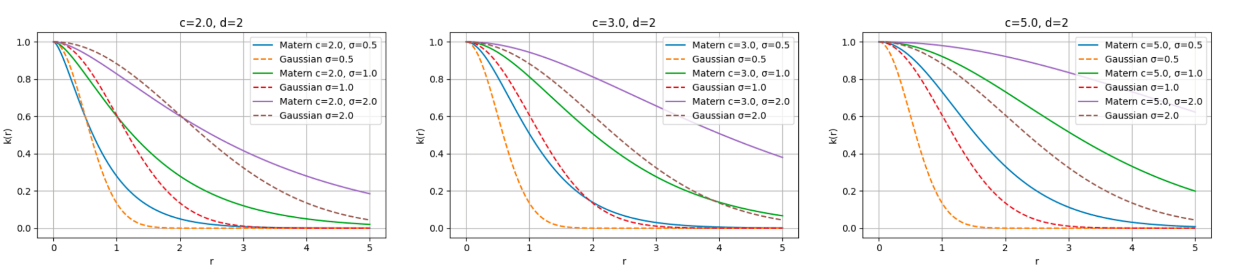
\(L=\alpha^{-1}(\mathrm{Id}-\sigma^2\Delta)^c\) \(k(r)=\alpha\frac{2^{1-\nu}}{\Gamma(\nu)}\left(\frac{r}{\sigma}\right)^\nu K_\nu\left(\frac{r}{\sigma}\right)\)
\(a(r)=\alpha^2 2^{\frac{3d}{2}-2c+1}\pi^{d/2}\sigma^d\frac{\Gamma(c)^2}{\Gamma(c-\frac{d}{2})^2\Gamma(2c)}\left(\frac{r}{\sigma}\right)^{2c-\frac{d}{2}}K_{2c-\frac{d}{2}}\left(\frac{r}{\sigma}\right)\)
Landmark shape spaces
Quotient space:
- stratification
- \(\mathfrak{se}(d)\) tangent action
- covectors and lifts
Metric:
- \(\pi\circ\mathrm{ev}_{s_0}\) a (stratified) Riemannian submersion
- cometric and CPD kernels
- geodesics
- constraint preservation and geodesic completeness
\(G\stackrel{\mathrm{ev}_{s_0}}{\longrightarrow}\mathrm{Land}^n(\mathbb R^d)\stackrel{\pi}{\longrightarrow}\mathrm{Land}^n(\mathbb R^d)/\mathrm{SE}(d)\)
Quotient, covectors, and normalization





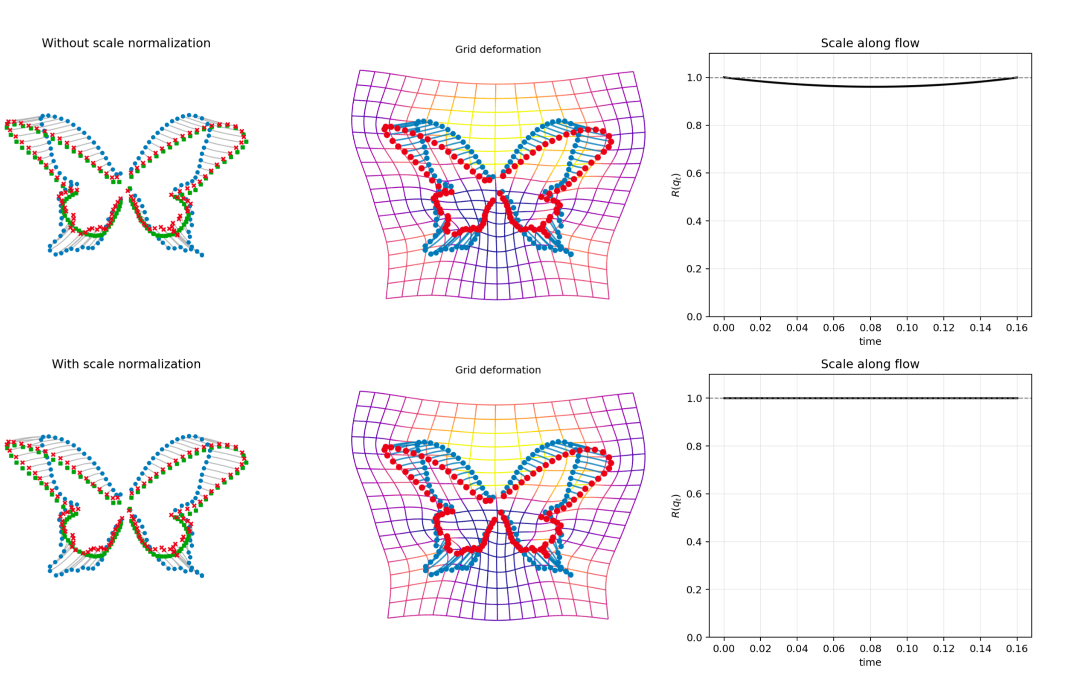
\(n\ge d\): Top stratum \(\mathcal{S}_k\) connected, open and dense
Size normalization:
Metric, screened elasticity
Metric induced by quadratic form \(\int_{\mathbb R^d}\langle Lv,v\rangle dx\) on \(\mathfrak{g}\subset\mathfrak X(\mathbb R^d)\)
- \(L\) equivariant to the action (conjugation) of \(\mathrm{SE}(d)\) on \(\mathrm{Diff}(\mathbb R^d)\)
- \(L\) can have null space \(\subseteq\mathfrak{se}(d)\)

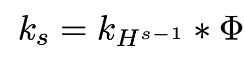

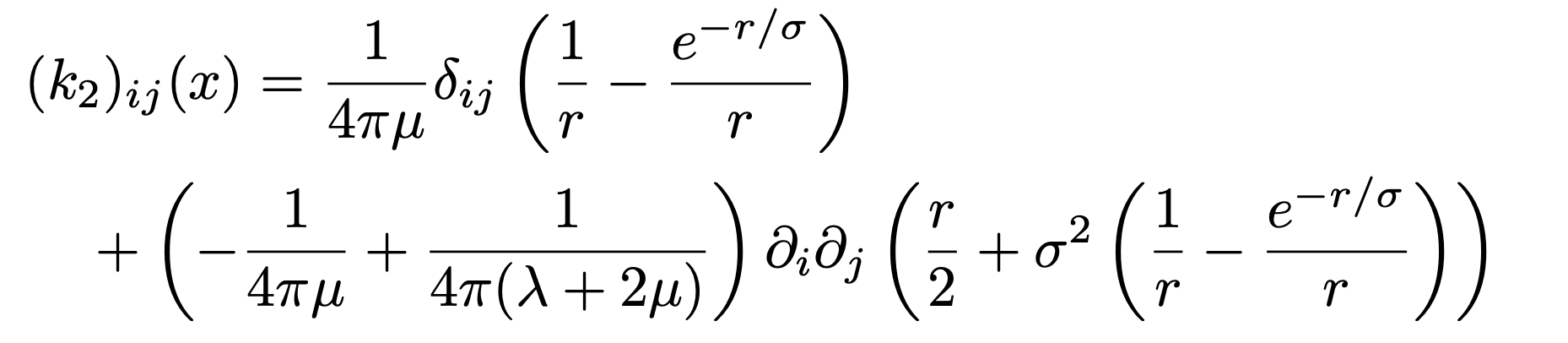
screening elasticity
\(\mathbb R^2\):
\(\mathbb R^3\):
operator:
Green's kernel:
(co-)Metric

Quadratic form
is positive for covectors satisfying
i.e., \(k_s\) is conditionally positive definite wrt. \(\mathfrak{se}(d)\),
positive definite on \(\mathfrak{se}(d)(q)^{\mathrm{ann}}\) and descends to a metric on \(\overline{\mathrm{Land}}^n\)
Lifts to \(\mathfrak{g}\):



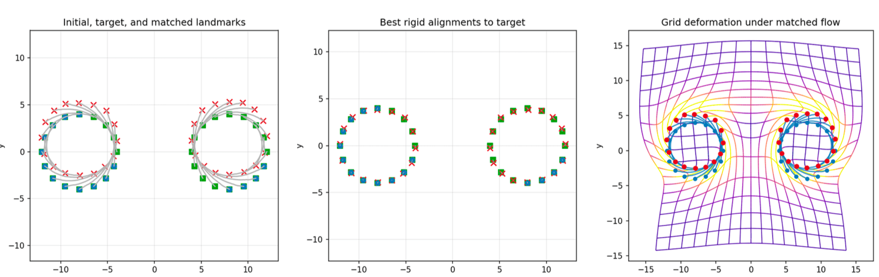
Geodesics

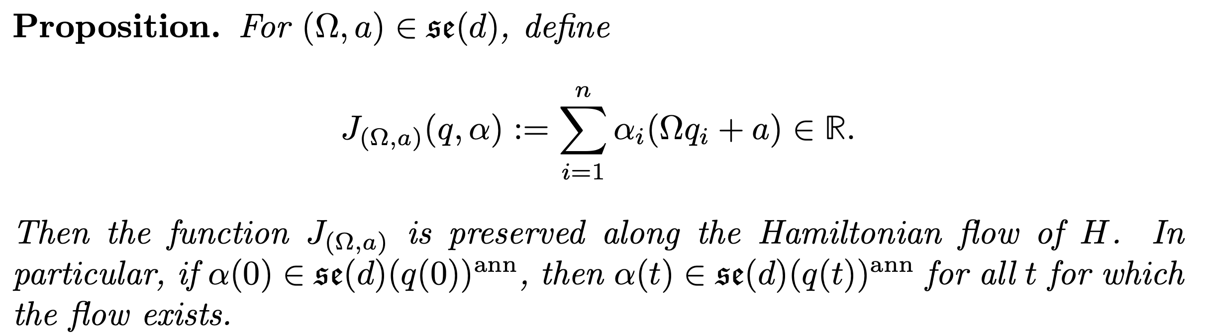

Hamiltonian:
Local rigid motion preservation
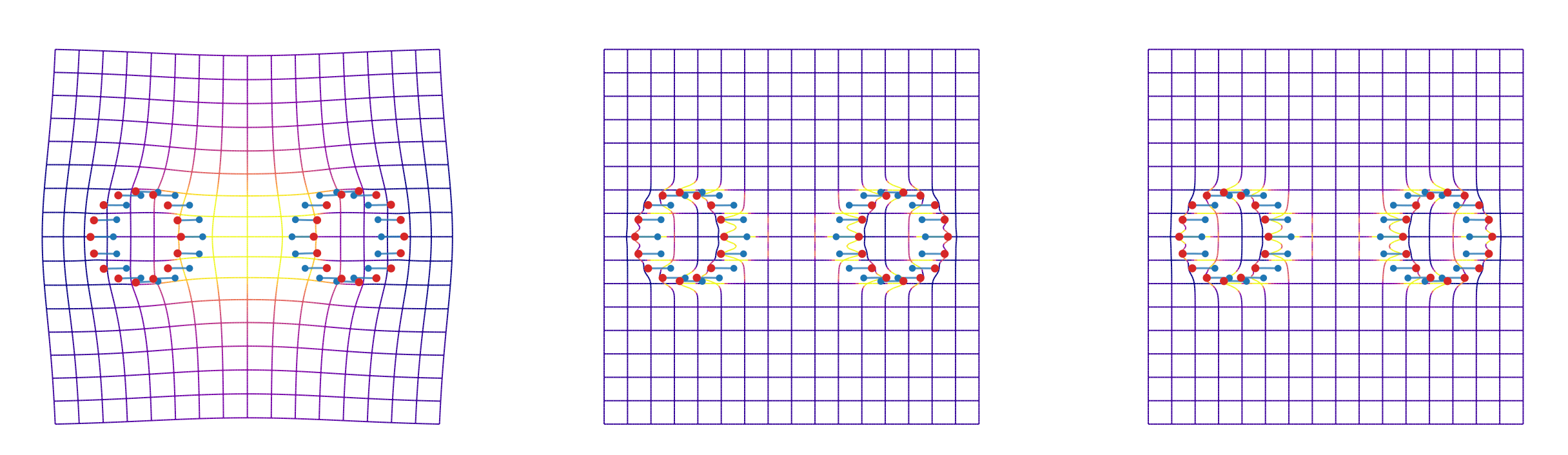
\(k_2\) Matern Gaussian
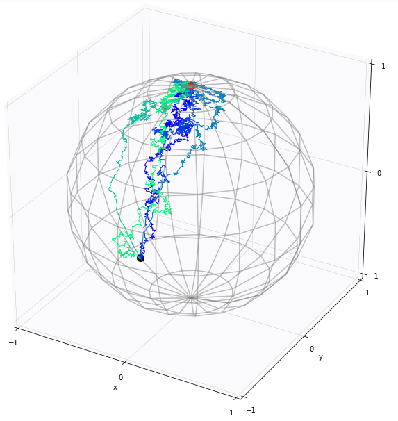
Inference: Data conditional processes
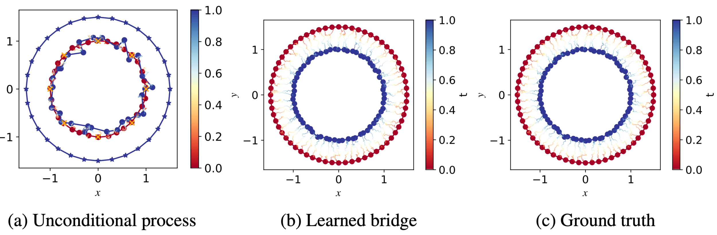
- \(X_t\) generates distribution \(p_t(\cdot|X_0)\)
- given observed shape \(v\), we wish for \(T>0\) to generate \(X_t|X_T=v\) - a bridge
\(X_t\) (no conditioning)
\(X_t|X_T=v\) (conditioned)
Bridges - conditional processes
- forward SDE:
\[dx_t = b(t,x_t)\,dt + \sigma(t,x_t)\,dW_t\] - conditioning to hit \(v\) at time \(T\) gives
new measure \(\mathbb{P}^*\):
\[\frac{d\mathbb{P}^*}{d\mathbb{P}}\Big|_{\mathcal{F}_t}= \frac{p(v,T\mid x_t,t)}{p(v,T\mid X_0,0)}\] - Doob's \(h\)-function: \(h(t,x) = p(v,T \mid x,t)\)
- SDE of \(\mathbb{P}^*\):
\[dx_t = \big[b(t,x_t) +a(t,x_t)\nabla_x \log \rho(x_t,t)\big]dt + \sigma(t,x_t)\,dW_t\]\(a(t,x)=\sigma\sigma^\top(t,x)\), \(\rho(x,t)=p(v,T\mid x,t)\) - the score \(\nabla_x \log \rho(x,t)\) steers trajectories to hit \(v\) at \(T\)
Score learning
- learn the score \( \nabla_x \log p(x,t) \) of the forward diffusion
-
fit neural network \( s_\theta \) to minimize
\[\mathcal{L}(\theta)= \frac{1}{2} \sum_{m=1}^M \int_{t_{m-1}}^{t_m}\left[\big\| s_\theta(t, x_t)-\nabla\log p(x_{t},t\mid x_{t_{m-1}},t_{m-1})\big\|_{a(t,x_t)}^2\right] dt\] -
plug \( s_\theta \) into SDE to sample: \[ dx_t = b(t,x_t)dt +a(t,x_t)s_\theta(t,x_t) dt + \sigma(t,x_t)\,dW_t \]
- +: scalable training from unconditioned data; no bridge likelihoods needed.
- -: can be hard to train in practice, rare-event bridges poorly covered, parameter dependence
Infinite dimensions and score learning
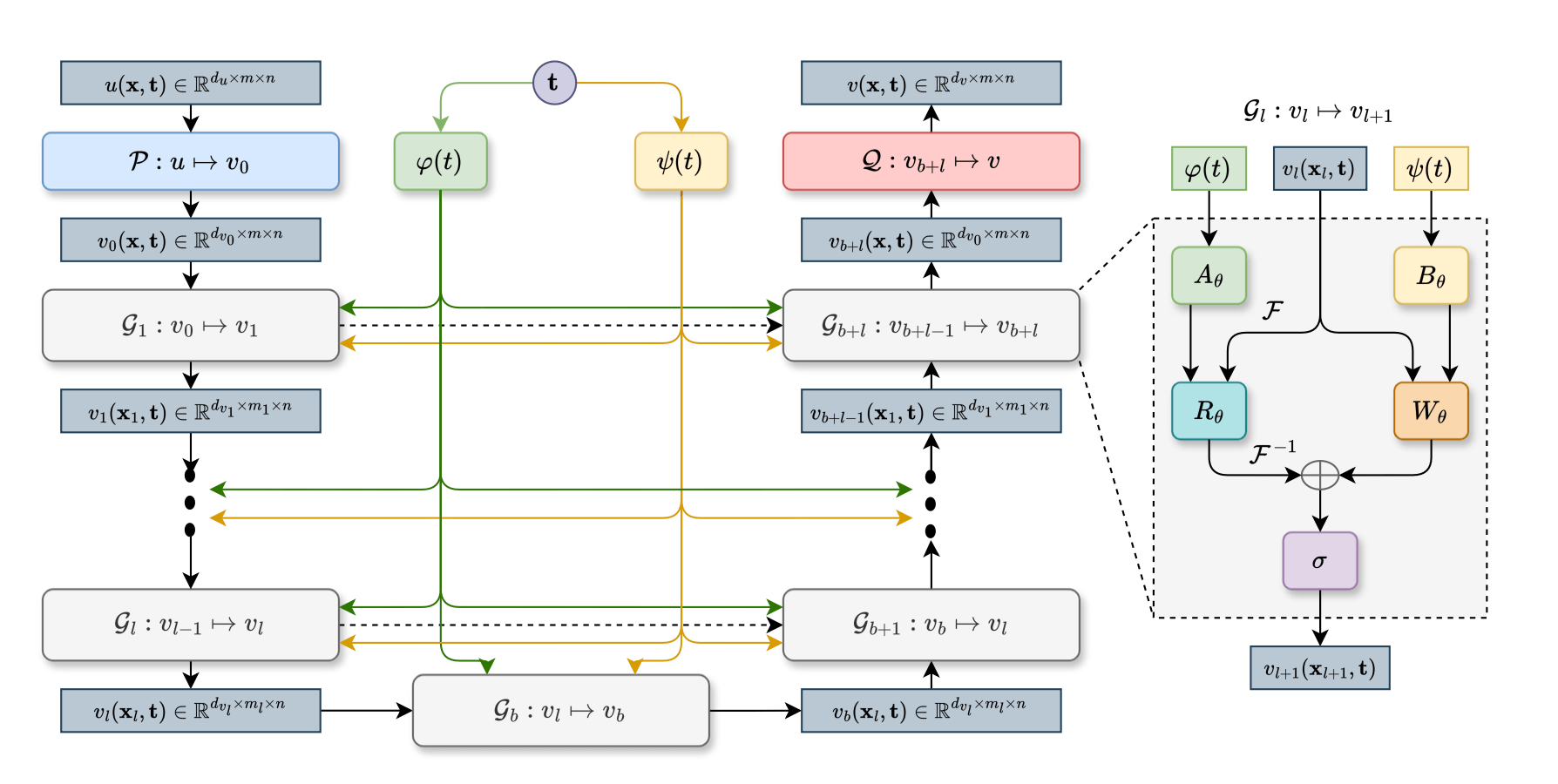
Train a neural network to learn the score in the bridge SDE in inf. dim.
\[dx_t=b(t,x_t)dt+a(t,x_t)\nabla_x\log \rho(t,x_t)dt\\+\sigma(t,x_t)dW_t\]particularly for shape Kunita flows
Auxilary process:
\[d\tilde{x}_t=\tilde{b}(t,\tilde{x}_t)dt+\tilde{\sigma}(t,\tilde{x}_t)dW_t\]
Approximate bridge:
\[dx_t^\circ=b(t,x_t^\circ)dt+a(t,x_t^\circ)\nabla_x\log \tilde{\rho}_t(x_t^\circ)dt\\+\sigma(t,x_t^\circ)dW_t\]
for e.g. linear processes, score \(\nabla_x\log \tilde{\rho}_t\) is known in closed from
(almost) explicitly computable likelihood ratio:
\[\frac{d\mathbb P^*}{d\mathbb P^\circ}=\frac{\tilde{\rho}_T(v)}{\rho_T(v)}\Psi(x_t^\circ)\]
Backward filtering, forward guiding: van der Meulen, Schauer et al.
Ito stochastic process:
\[dx_t=b(t,x_t)dt+\sigma(t,x_t)dW_t\]
Bridge process:
\[dx^*_t=b(t,x^*_t)dt+a(t,x^*_t)\nabla_x\log\rho_t(x^*_t)dt\\+\sigma(t,x^*_t)dW_t\]
Score \(\nabla_x\log \rho_t\) intractable, but ...
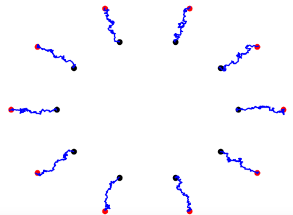
Backwards filtering, forward guiding bridges
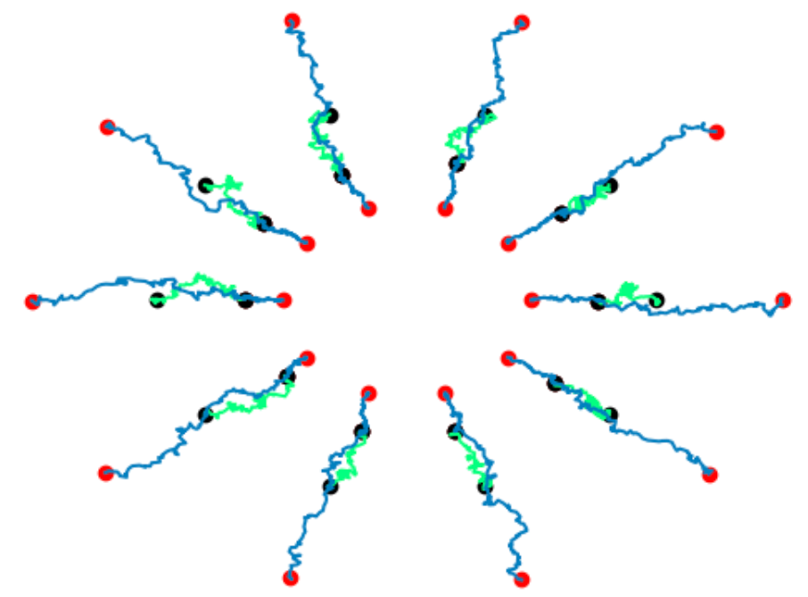
From single edges to trees
Bridge:
Leaf conditioning:
\(x_0\)
\(v\)
\(x_0\)
\(h\)
\(v_1\)
van der Meulen, Schauer'20; van der Meulen'22
Stoustrup, Nielsen, van der Meulen, Sommer
\(v_2\)
recursive,leaves to root
Backwards filter:
root to leaves
Forward guiding:
\(v\)
\(v_1\)
\(v_2\)
\(h\)
\(x_0\)
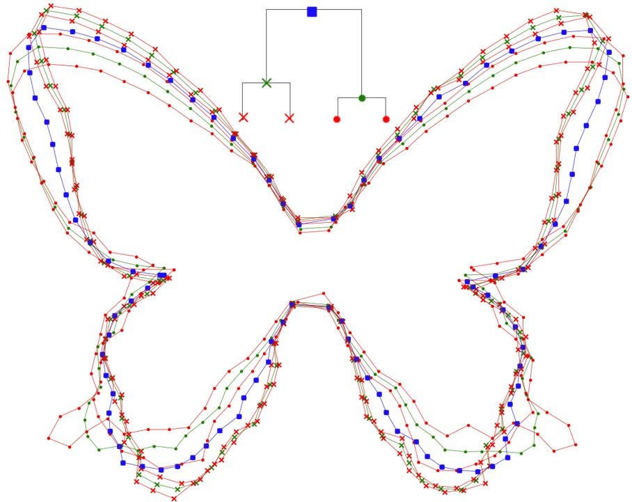
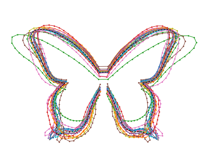
Backwards filtering, forward guiding butterflies
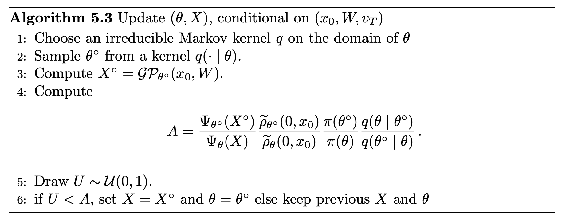
v.d. Meulen,Schauer,Sommer,'25
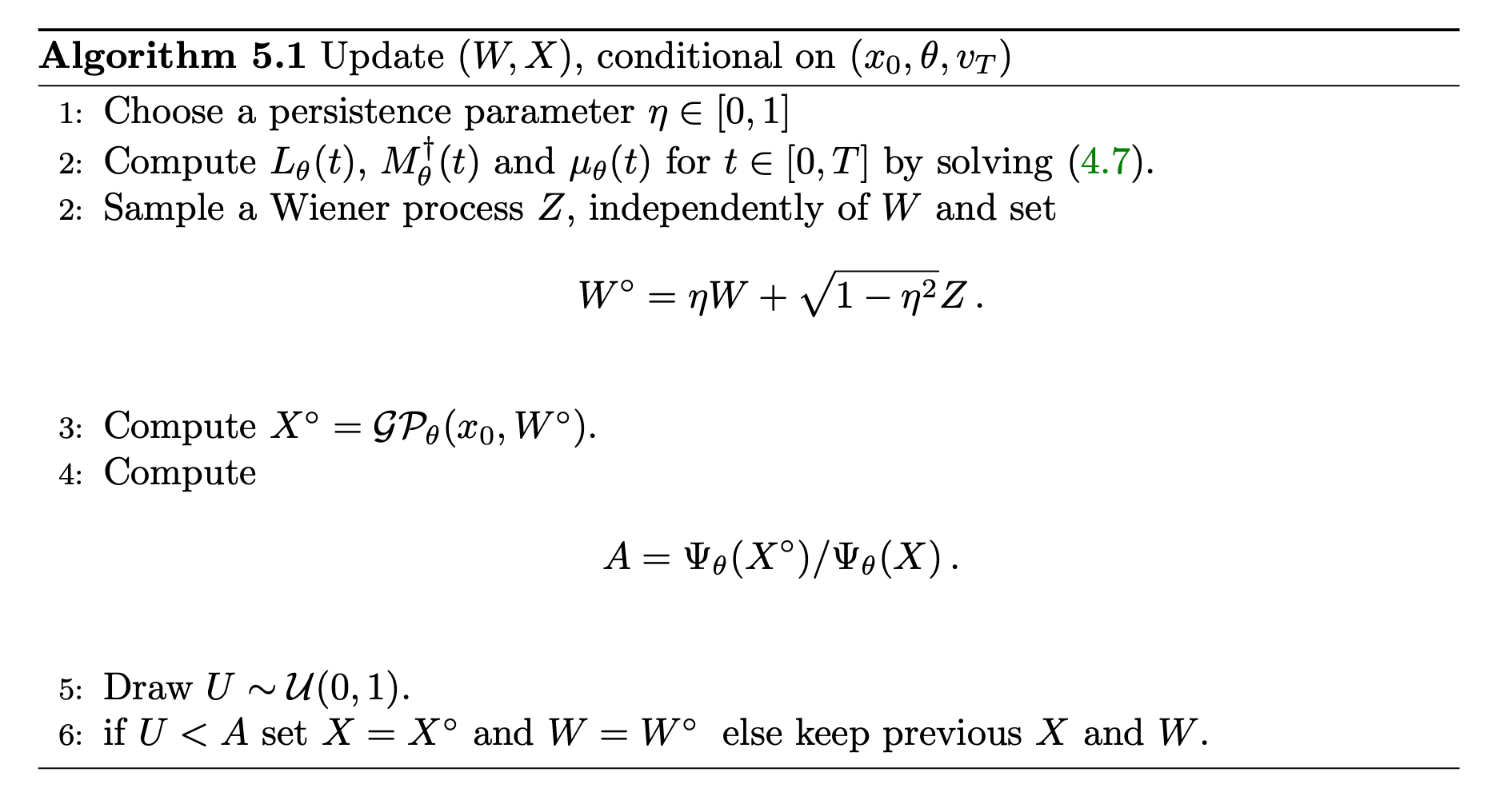
Parameter inference with MCMC
sample parameters (e.g. kernel width, amplitude)
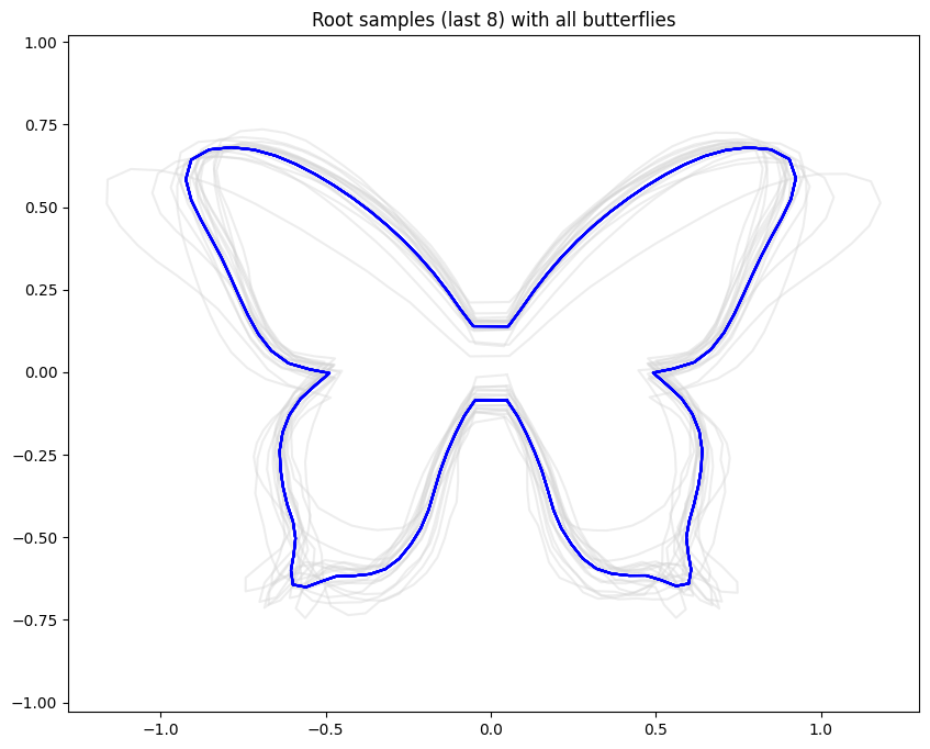
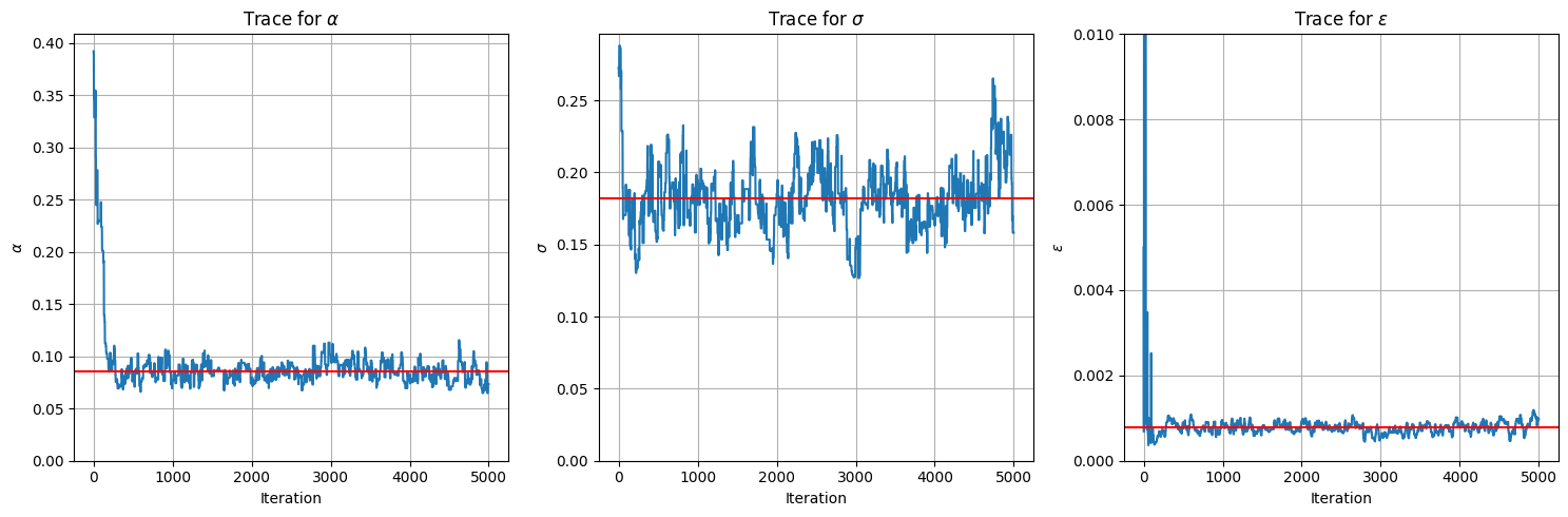
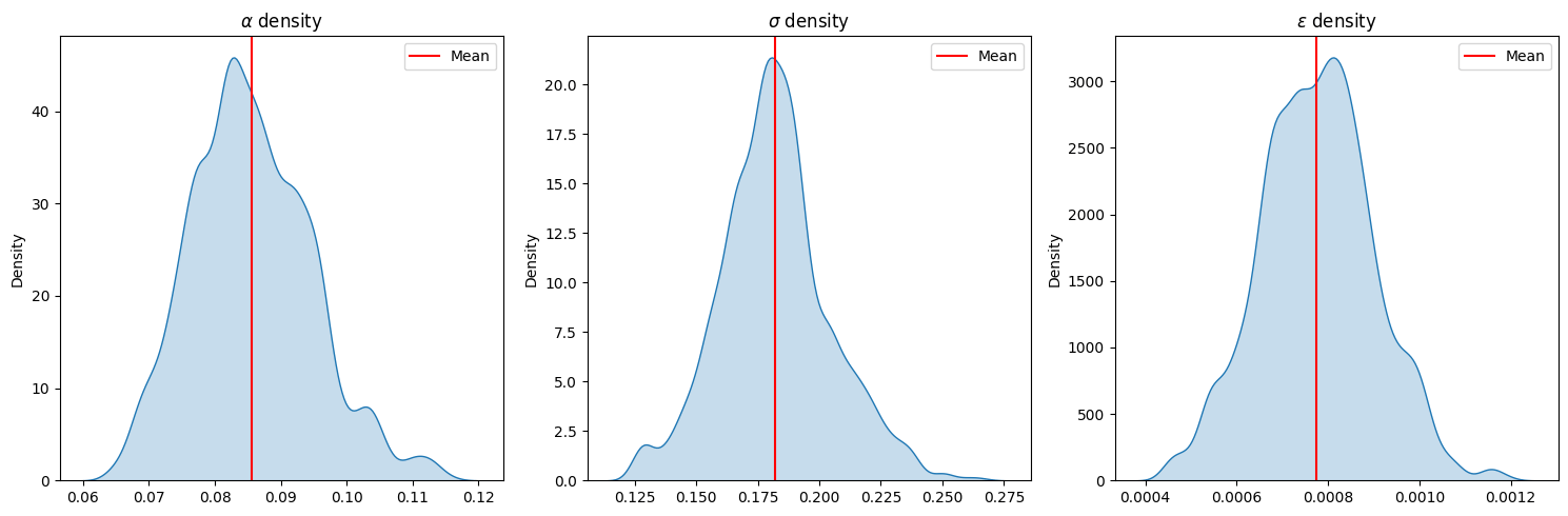
v.d. Meulen,Schauer,Arnaudon,Sommer,SIIMS'22
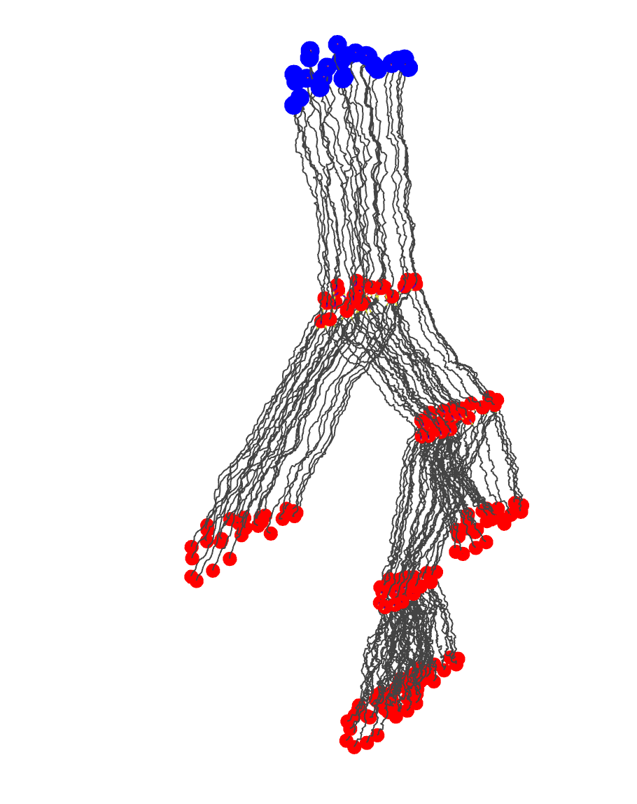
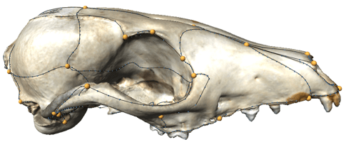
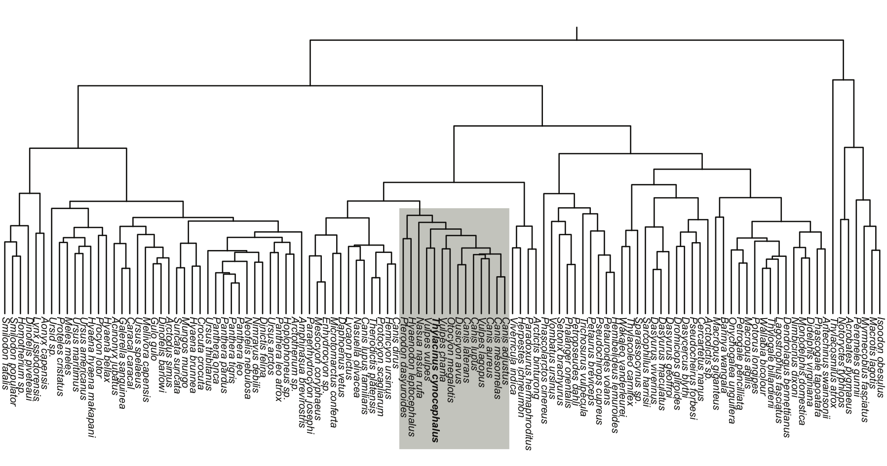
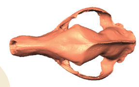
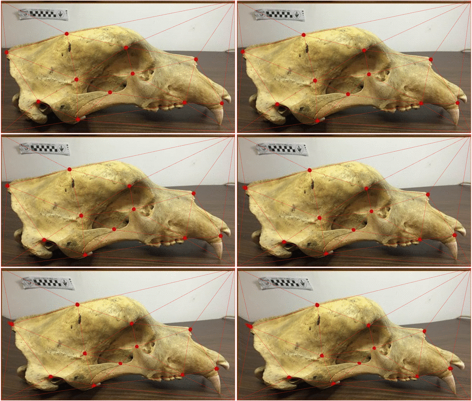
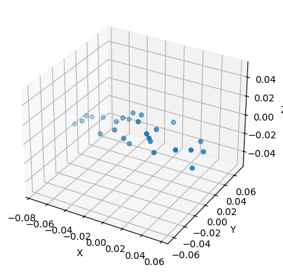
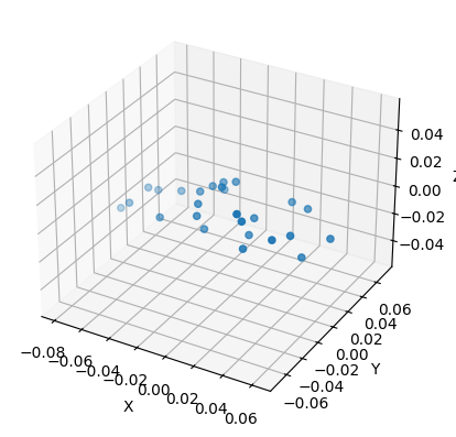
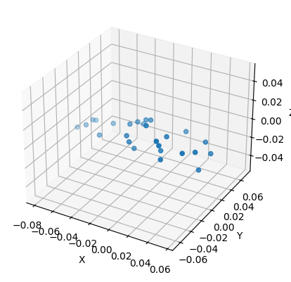
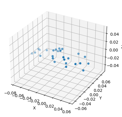
Canidae skulls
Severinsen, Hipsley, Nielsen, Sommer
Neural guided diffusion bridges
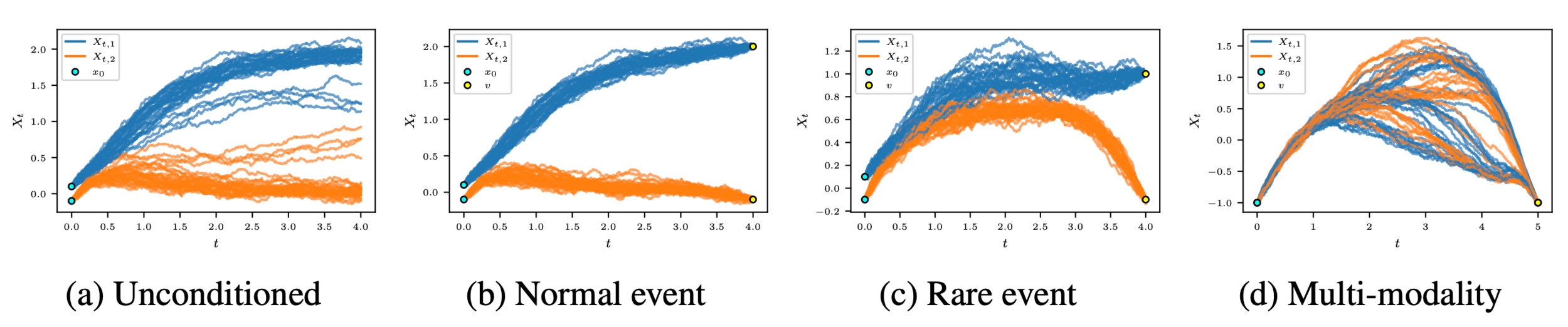
Yang,van der Meulen,Sommer,ICML'25
- in addition to guide \(a(t,x_t)\tilde r(t,x_t)\) to \(b(t,x_t)\), further inject a learnable control \(\sigma(t,x)\vartheta_\theta(t,x)\):
\[dx_t = \big[b(t,x_t) + a(t,x_t)\tilde r(t,x_t) + \sigma(t,x_t)\vartheta_\theta(t,x_t)\big]dt\\ + \sigma(t,x_t)\,dW_t\] - \(\vartheta_\theta\) is a bounded neural net that approximates the missing score-like drift \(r^\star - \tilde r\), steering the guided process toward the exact bridge
- training minimizes the loss
\[L(\theta) = \mathbb{E}\!\int_0^T \left[\tfrac12\|\vartheta_\theta(t,x_t)\|^2 - G(t,x_t)\right]dt,\] where \(G\) encodes drift/diffusion mismatches - when \(L(\theta)\) is minimized, independent bridges draw as cheaply as the forward SDE, no MCMC-based guides or unconditional score learning.
Landmark shape spaces and Kunita flows
JaxGeometry: https://github.com/computationalevolutionarymorphometry/jaxgeometry CCEM: http://www.ccem.dk
Hyperiax: https://github.com/computationalevolutionarymorphometry/hyperiax slides: https://slides.com/stefansommer
References:
- Yang, v. d. Meulen, Sommer: Neural backwards filtering forward guiding, https://arxiv.org/abs/2601.23030
- Sommer, Yang, Baker: Stochastics of shapes and Kunita flows, https://arxiv.org/abs/2512.11676
- Grong, Sommer: Most probable paths for developed processes, https://arxiv.org/abs/2211.15168
- Grong, Sommer: Most probable flows for Kunita SDEs, https://arxiv.org/abs/2209.03868
- Sommer, Schauer, v. d. Meulen: Stochastic flows and shape bridges, Oberwolfach, 2021
- Baker, Besnier, Sommer: A function space perspective on stochastic shape evolution, https://arxiv.org/abs/2302.05382
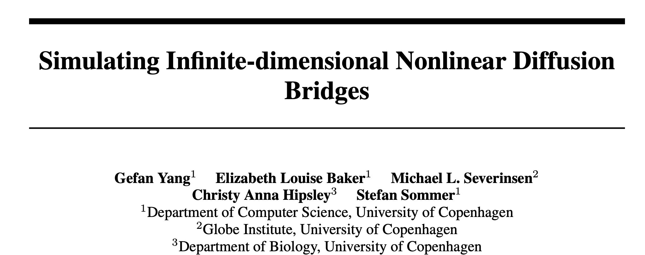
- Yang, Baker, Severinsen, Hipsley, Sommer: Simulating infinite-dimensional nonlinear diffusion bridges, https://arxiv.org/abs/2405.18353
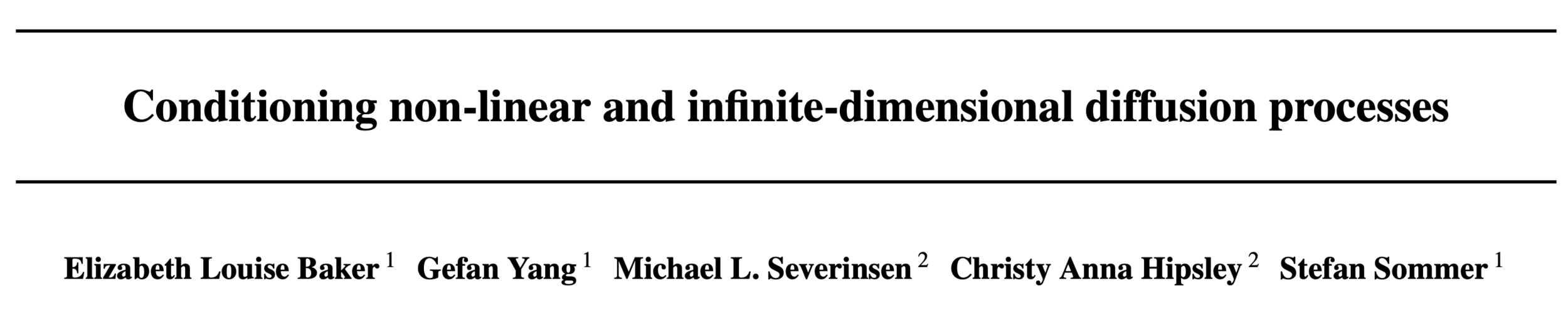
- Baker, Yang, Severinsen, Hipsley, Sommer: Conditioning non-linear and infinite-dimensional diffusion processes, https://arxiv.org/abs/2402.01434
- Hansen, Eltzner, Huckemann, Sommer: Diffusion Means in Geometric Spaces, Bernoulli, 2023, arXiv:2105.12061
- Grong, Sommer: Most probable paths for anisotropic Brownian motions on manifolds, FoCM 2022, arXiv:2110.15634
- Philipp Harms, Peter W. Michor, Xavier Pennec, Stefan Sommer: Geometry of sample spaces, Diff. Geom. and its Appl., 2023, arXiv:2010.08039
- Arnaudon, v.d. Meulen, Schauer, Sommer: Diffusion bridges for stochastic Hamiltonian systems and shape evolutions,SIIMS,2022,arXiv:2002.00885
- Højgaard Jensen, Sommer: Simulation of Conditioned Diffusions on Riemannian Manifolds, 2021, arXiv:2105.13190.
- Arnaudon, Holm, Sommer: A Geometric Framework for Stochastic Shape Analysis, Foundations of Computational Mathematics, 2019, arXiv:1703.09971.
- Sommer, Svane: Modelling Anisotropic Covariance using Stochastic Development and Sub-Riemannian Frame Bundle Geometry, JoGM, 2017, arXiv:1512.08544.
- Arnaudon, Holm, Sommer: A Stochastic Large Deformation Model for Computational Anatomy, IPMI 2017, arXiv:1612.05323.