Linear Systems
Numerical Methods
David Mayerich
Scalable Tissue Imaging and Modeling (STIM) Laboratory
Department of Electrical and Computer Engineering
Cullen College of Engineering
University of Houston
David Mayerich
STIM Laboratory, University of Houston

Linear Equations
David Mayerich
STIM Laboratory, University of Houston
Loop Currents with Kirchhoff's Laws
David Mayerich
STIM Laboratory, University of Houston
Solutions to Linear Systems
-
Linear systems take the form: \(\mathbf{Ax}=\mathbf{b}\)
-
The purely analytical solution is: \(\mathbf{A}^{-1}\mathbf{b}=\mathbf{x}\)
where \(\mathbf{A}^{-1}\) is the inverse of \(\mathbf{A}\) -
Options for solving \(\mathbf{x}\) include:
-
Calculate \(\mathbf{x}\) using a direct method (ex. Gaussian Elimination)
-
Calculate \(\mathbf{x}\) using an indirect (often iterative) method
-
Calculate \(\mathbf{A}^{-1}\) and multiply: \(\mathbf{x} = \mathbf{A}^{-1}\mathbf{b}\)
-
-
We will cover each of these options, starting with direct methods
David Mayerich
STIM Laboratory, University of Houston
Gaussian Elimination
Row Reduction
Algorithm
Back Substitution
David Mayerich
STIM Laboratory, University of Houston
Gaussian Elimination
-
Gaussian elimination is a 2-step algorithm for directly computing \(\mathbf{x}\)
-
Convert the augmented matrix \(\left[\mathbf{A}|\mathbf{b}\right]\) to row-eschelon form
-
Perform back-substitution to calculate the scalar values of \(\mathbf{x}\) from bottom to top
David Mayerich
STIM Laboratory, University of Houston
-
Row-eschelon form:
-
Rows with non-zero elements are above rows with all zeros
-
The leading coefficient of row \(k\) is to the right of the leading coefficient of \(k-1\)
-
All values in a column below a leading coefficient are zero
-
Row Reduction
-
Assuming \(\mathbf{A}\in\mathbb{R}^{n\times n}\) and \(\mathbb{b}\in \mathbb{R}^{N}\), build the augmented matrix \(\mathbf{C} = \left[\mathbf{A}|\mathbf{b}\right] \in \mathbb{R}^{n \times (n+1)}\)
-
For each row \(i \in \mathbb{N}\) in the matrix
- For each row \(\{k\in\mathbb{N}|k>i \land k < n\}\) below row \(i\)
- Calculate a value \(s = \frac{a_{k, p}}{a_{k, k}}\) (used to eliminate the coefficients under \(a_{k, k}\))
- Subtract the scaled row \(i\) from row \(k\): \(r_i \leftarrow r_i - s r_k\)
- For each row \(\{k\in\mathbb{N}|k>i \land k < n\}\) below row \(i\)
David Mayerich
STIM Laboratory, University of Houston
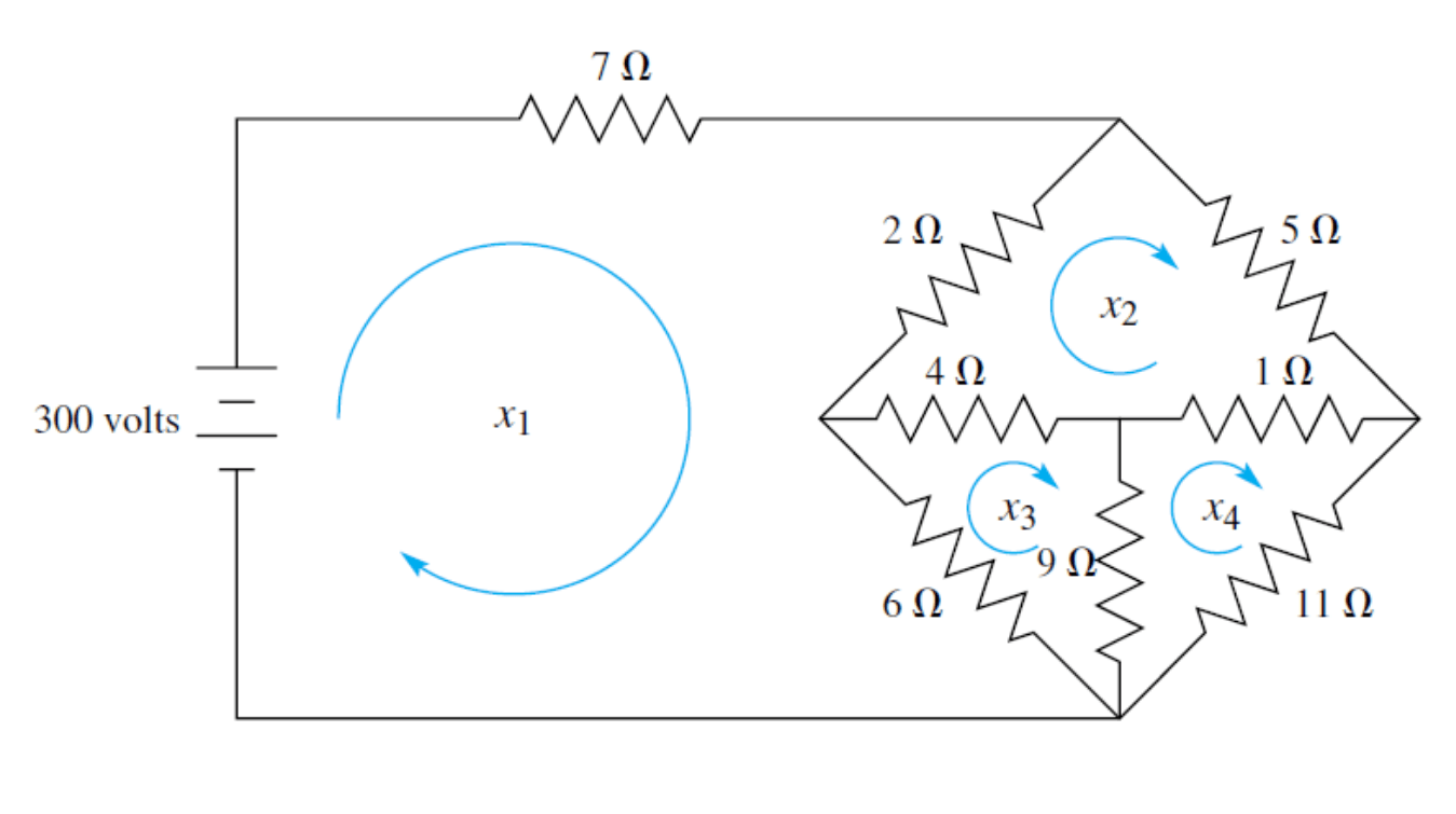
Loop Currents (Row 1)
David Mayerich
STIM Laboratory, University of Houston
Loop Currents (Row 2)
David Mayerich
STIM Laboratory, University of Houston
Loop Currents (Row 3)
David Mayerich
STIM Laboratory, University of Houston
Gaussian Elimination Algorithm
David Mayerich
STIM Laboratory, University of Houston
gaussian(double* A, double* b, int N){
  for(int k=0; k<N-1; k++){ 		// for each pivot
    for(int i=k+1; i<N; i++){ 		// for each equation
      float m=A[i*N+k] / A[k*N+k]; 	// calculate scale
      for(int j=k; j<N; j++){ 		// for each coefficient
        A[i*N+j] -= m * A[k*N+j]; 	// subtract
      }
      b[i] -= m * b[k]; 			// forward elimination
    }
  }
}-
What is the computational complexity?
Back Substitution
David Mayerich
STIM Laboratory, University of Houston
Back Substitution - Algorithm
David Mayerich
STIM Laboratory, University of Houston
backsub(double* A, double* b, double* x, int N){
  x[N-1] = b[n-1] / A[(n-1)*N+n-1];	// calculate 𝑥𝑛
  for(int i=N-2; i>=0; i--){ 		// for each equation
    float sum = b[i]; 				// start a sum
    for(int j=i+1; j<N; j++){ 		// for each coefficient
      sum+=A[i*N+j] * x[j]; 		// add coeffs and knowns
    }
    x[i]=sum/A[i*N+i]; 				// calculate 𝑥𝑖
  }
}-
What is the computational complexity?
-
Total complexity: \(O\left(n^3\right) + O\left(n^2\right) = O\left(n^3\right)\)
Loss of Precision
Testing Gaussian Elimination
Geometric Series
Compounding Errors
David Mayerich
STIM Laboratory, University of Houston
Testing Gaussian Elimination
-
We can test robustness by creating an artificial problem
-
Consider the geometric series:
David Mayerich
STIM Laboratory, University of Houston
-
A geometric series has an analytical solution:
where \(2\leq t \leq n+1\)
-
Try to recover the coefficient \(a\) for an \(n\)th order geometric series given \(n\) equations
-
For each equation:
\(a=1\) and \(t_i=1+i\) where \(i=1\) to \(n\)
Linearized Geometric Series
David Mayerich
STIM Laboratory, University of Houston
Geometric Series Example
-
For \(3\) equations \((n=3)\) and coefficient \(a=1\):
David Mayerich
STIM Laboratory, University of Houston
-
For \(4\) equations \((n=4)\) and coefficient \(a=1\):
Testing Gaussian Elimination
-
Now we can test the robustness of the algorithm by adjusting \(n = 4, 5, 6, 7, \cdots\)
-
Compare the result vector \(x\) to the known values \(\mathbf{x}=[1, 1, \cdots, 1]^T\)
-
Using Gaussian Elimination to solve this system:
-
Precise results up to \(n=9\)
-
At \(n=9\), one result has a relative error \(\epsilon_r = 16,000\%\)
-
-
Next, we will discuss why this happens
David Mayerich
STIM Laboratory, University of Houston
Errors
-
Consider the following linear system:
David Mayerich
STIM Laboratory, University of Houston
-
First step of Gaussian elimination results in division by zero
-
If a numerical method fails for some value, it might be unstable near that value
Rounding Errors
-
Take a linear system involving some small number \(\epsilon\):
David Mayerich
STIM Laboratory, University of Houston
-
What is the correct answer?
-
What will you actually get?
Rounding Errors
-
Row reduction:
David Mayerich
STIM Laboratory, University of Houston
-
Backsubstitution:
-
If \(\frac{1}{\epsilon}\) is large, then both \(\left(2 - \frac{1}{\epsilon}\right)\) and \(\left(1 - \frac{1}{\epsilon}\right)\) approach \(-\frac{1}{\epsilon}\)
Numerical Demonstration
-
Solve the following linear system keeping \(4\) significant figures
David Mayerich
STIM Laboratory, University of Houston
correct values
Rounding Errors - 2nd Example
-
This issue doesn't just happen when one coefficient is small
-
The problem is when one coefficient is small relative to other coefficients in the row
David Mayerich
STIM Laboratory, University of Houston
-
Row reduction:
-
Back substitution:
correct values