Lecture 8:
Continuous Control
Artyom Sorokin | 13 Apr
Continuous Action Spaces

Deep RL Family Tree:
DQN
Many DQN variants
Policy Gradient
A2C/A3C
REINFORCE/PG+
TRPO
PPO
Value-Based
Policy-Based
Deep RL Family Tree:
Off-Policy
DQN
Many DQN variants
Policy Gradient
A2C/A3C
REINFORCE/PG+
TRPO
PPO
Close to On-Policy
On-Policy
Value-Based
Policy-Based
Deep RL Family Tree:
- Off-Policy
DQN
Many DQN variants
Policy Gradient
A2C/A3C
REINFORCE/PG+
TRPO
PPO
- Close to On-Policy
- On-Policy
Value-Based
Policy-Based
Discrete Actions:
Continuous Actions


Where are my off-policy methods for continuous actions?
Problem with Value-Based Methods
Value-Based methods learn to estimate \(Q(s,a)\)
How to get best action action from \(Q\)-values?
huge number of actions \(\rightarrow\) expensive
continuous action space \(\rightarrow\) solve optimization problem at each \(t\)
Why PG-based methods work:
Recall Policy Gradients (A2C version):
No need to estimate for (s, a) pairs
Simplest advantage function estimate:
Select actions from parametrized distribution family, e.g, Gaussian
Many version of PG formula:
Screen from GAE paper(arxiv.org/abs/1506.02438):

Which \(\Psi_{t}\) is suitable for continuous action spaces?
All of them!
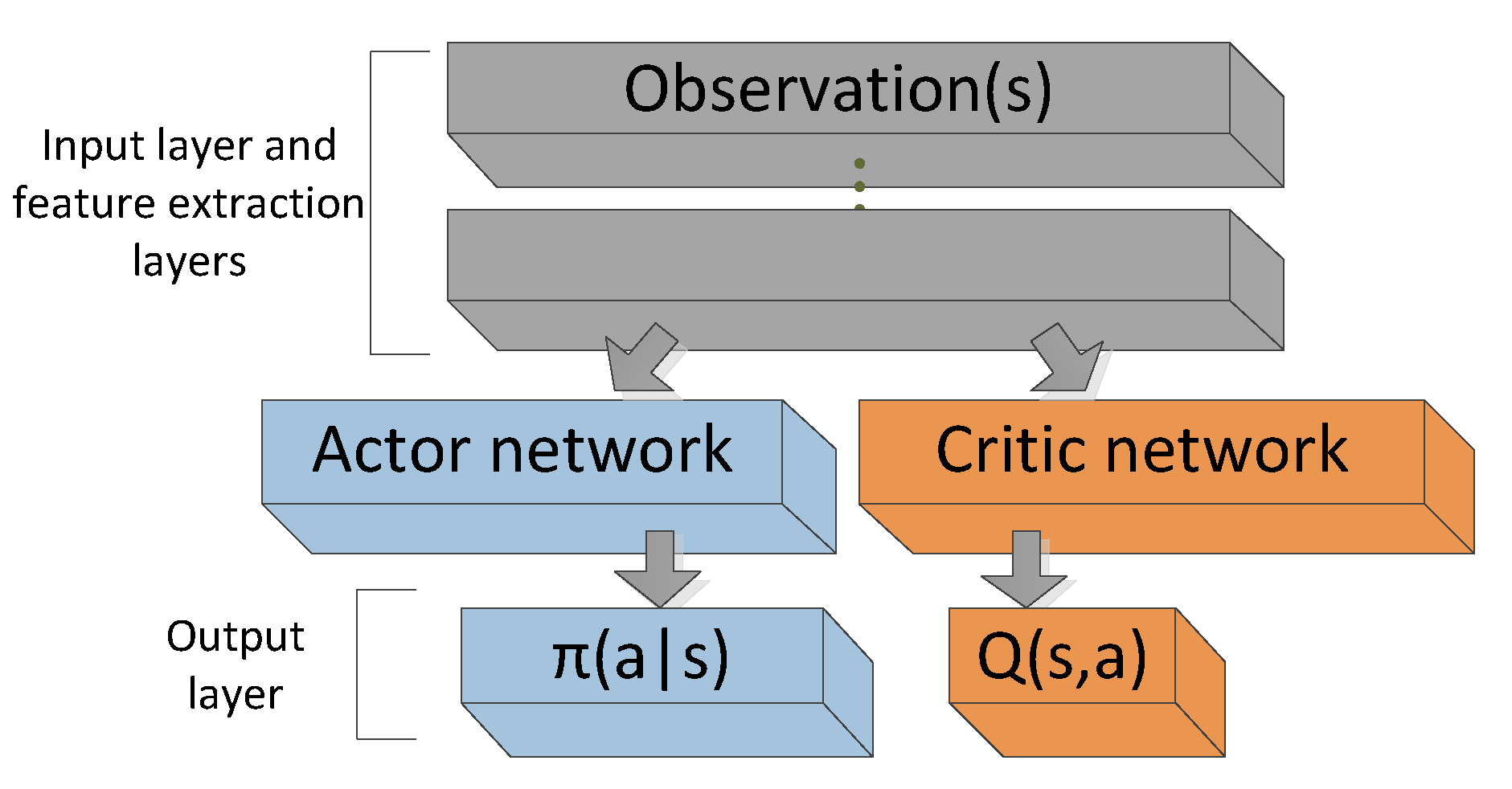
A2C with Q-values
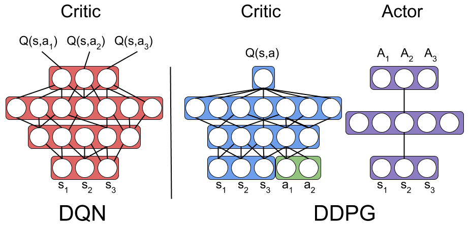
In discrete case we can just output all \(Q(s,a)\):
But we are interested only in \(Q\)-values for particular \(a_t\)!
A2C: Q-values + Continuous Actions
Continuous case: Estimate \(Q\)-values only for the selected action \(a_t\)
Conclusions:
- Explicit policy allows to omit the problem with \(argmax_{a}\) over all actions
- PG theorem proofs that this is a correct algorithm
Continuous case: Estimate \(Q\)-values only for the selected action \(a_t\)
One problem: PG is still on-policy!
DPG: Intro
Idea:
- Learn Q-values off-policy with 1-step TD-updates
- Gradients \(\nabla_{a} Q_{\phi}(s,a)\) tell how to change the action \(a \sim \pi(s)\) to increase \(Q\)-value
- Update actor with these gradients!
Problems:
- Can't flow gradients via sampled actions!
- Do we have any justifications for this?
Use deterministic policy ¯\_(ツ)_/¯
Yes! For deterministic policy :)
Deterministic Policy Gradients:
Now we can rewrite RL objective (Recall PG lecture):
Lets start for new definitions:
- \(\rho_1(s)\): The initial distribution over states
- \(\rho(s \rightarrow s', k, \mu)\): starting from \(s\), the visitation probability density at \(s'\) after moving k steps with policy \(\mu\)
- \(\rho^{\mu}(s')\): Discounted state distribution, defined as:
Deterministic Policy Gradients:
Deterministic Policy Gradient Theorem:
where,
- \(\rho_1(s)\): the initial distribution over states
- \(\rho(s \rightarrow s', k, \mu)\): starting from \(s\), the visitation probability density at \(s'\) after moving k steps with policy \(\mu\)
- \(\rho^{\mu}(s')\): Discounted state distribution, defined as:
Deterministic Policy Gradients:
TODO! Choose one of Two types of Explanation:
Var1:
- DPG theorem proof
Var2:
- PG theorem with "improper" discounted \(\rho^{\pi}(s)\) as it easier
- Show part of DPG Theorem until we start telescoping
- Then DPG is similiar with PG only with integrals
DPG Proof V1

For more details see: DPG paper and supplementary materials
Notice that we also can rewrite \(J(\mu_{\theta})\) as:
And first we want to prove that:


DPG at first step
expectation over s'
V-value at next step
DPG Proof V1

Leibniz integral rule:
swap grad and integral
same
same
DPG Proof V1

linearity of gradients and integration
By Q-value definition!
by definition of \(p(s \rightarrow s', k, \mu_{\theta})\)
Deterministic Policy Gradient V1
This is proven:


Now we can recursively iterate with this formula for all steps:


until all \(\nabla _{\theta}V^{\mu_{\theta}}\) are gone!
Deterministic Policy Gradient V1
Now return to:
And substitute \(\nabla_{\theta} V^{\mu_{\theta}}\) with our new formula:
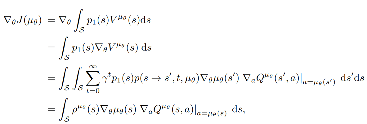
Leibniz integral rule
Fibini's theorem to swap integration order
Deterministic Policy Gradient:
Off-policy Policy Gradient theorem (arxiv.org/abs/1205.4839):
We can learn DPG off-policy:
- DPG version of Off-Policy PG Theorem allows to ignore importance sampling correction
- Learning Q-function with 1-step TD-learning allows to learn critic off-policy

Imporance sampling
recall TRPO, PPO derviations...
Deep Deterministic Policy Gradient
Mods inspired by DQN:
- Add noise(Ornstein-Uhlenbeck or Gaussian) to the sampling policy:
- Replay Buffer as in DQN
- Separate "deep" networks for Actor and Critic
- Target Actor and target Critic
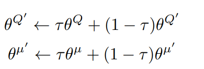
- Update target networks with moving average:
Lets combine DPG with Deep Learning and create DDPG!


DDPG Results
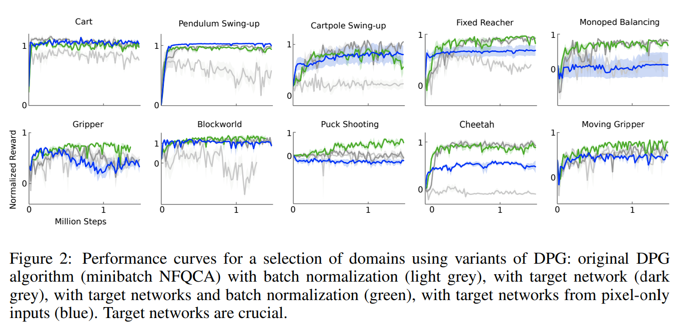
Twin-Delayed DPG
DDPG has many problems! Lets try to fix them!
Fix #1
Clipped Double Q-learning [ this is "twin" part ]:
- Train two Critic networks:
- Fight overestimation bias by taking minimum of the two targets:
DDPG has many problems! Lets try to fix them!


Twin-Delayed DPG
DDPG has many problems! Lets try to fix them!
Fix #2
Delayed update of Target and Policy Networks:
- Problem: policy updates is poor if value estimates are inaccurate
- Update Target Networks and Actor less frequently than Critic
DDPG has many problems! Lets try to fix them!
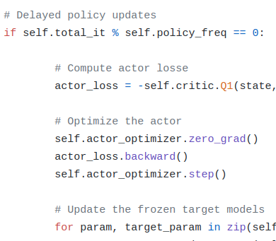
From author's code of TD3:
Twin-Delayed DPG
DDPG has many problems! Lets try to fix them!
Fix #3
Target Policy Smoothing [ No reference in the name :( ]
- Problem: Deterministic policies can overfit to narrow peaks/fluctuations in the value function
- Add noise to the Traget Policy's action to prevent this:
DDPG has many problems! Lets try to fix them!

Twin-Delayed DPG
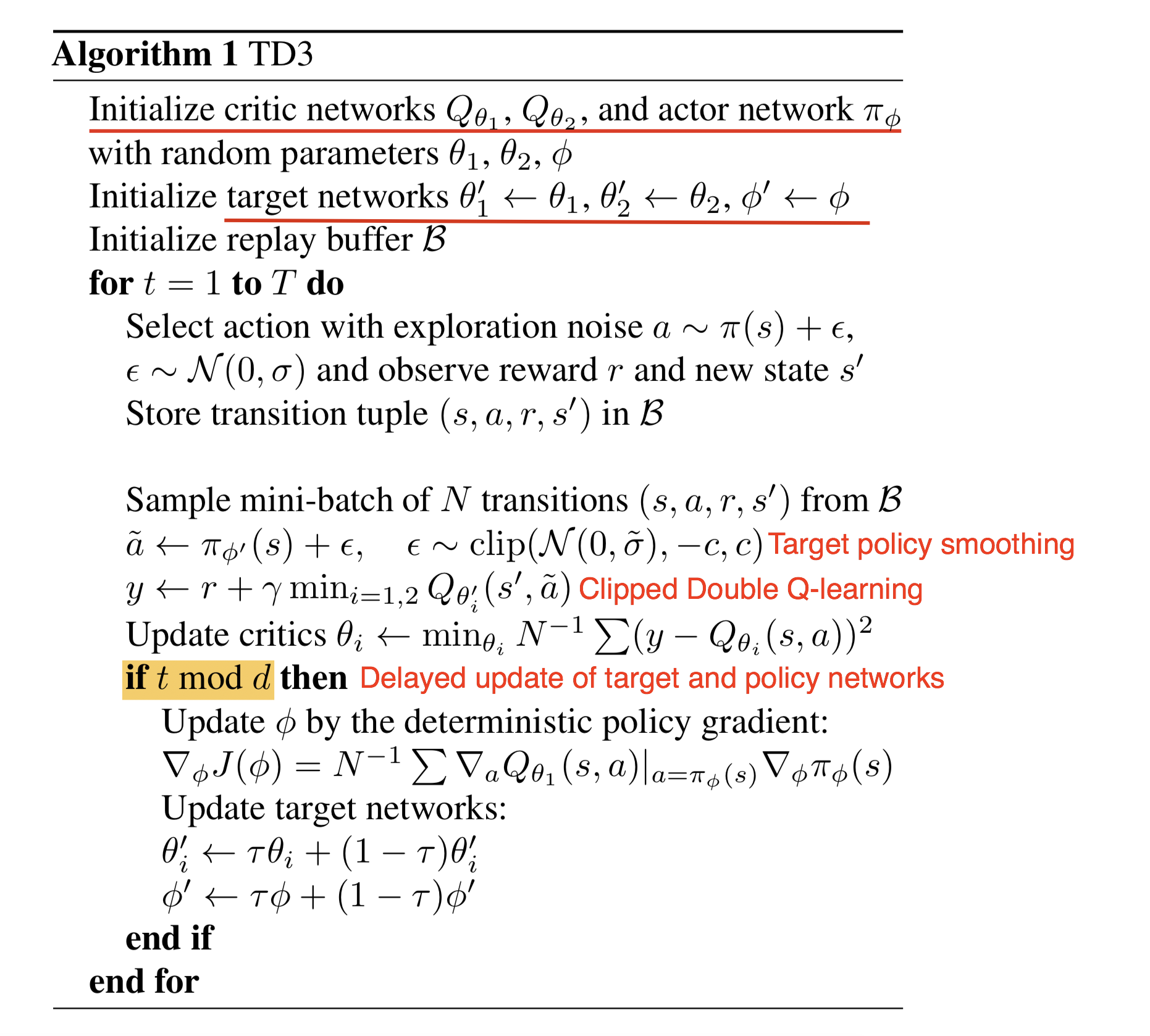
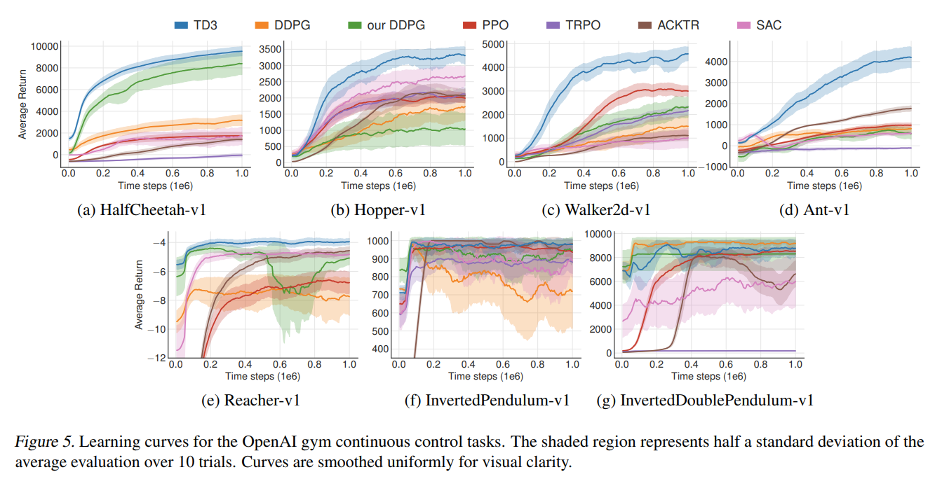
TD3: Results
Maximum Entropy RL
Max Entropy Objective:


Regular RL Objective:
Maximum Entropy RL
Backup Diagram:
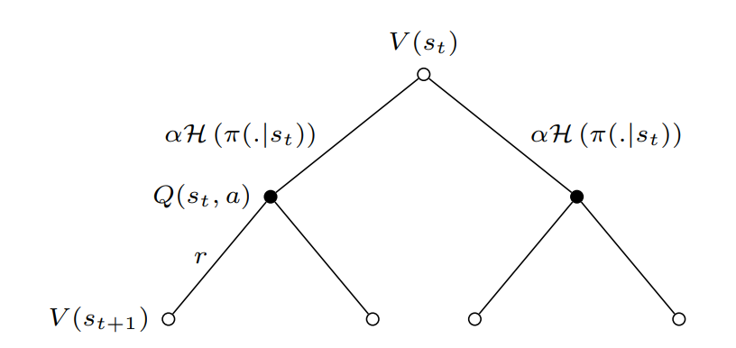

Add \(soft\) for every value function
Maximum Entropy RL
Maximum Entropy Bellman Operator:
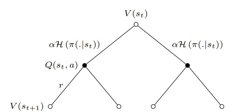

Maximum Entropy RL
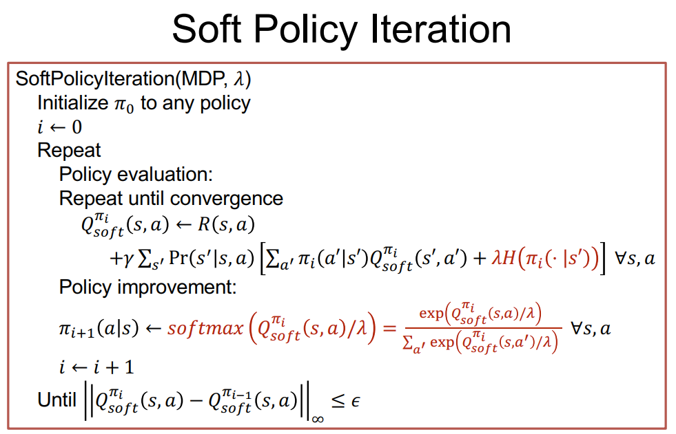
Why softmax over \(Q\)-values imporves policy?
Soft-PI: Intuition for Softmax
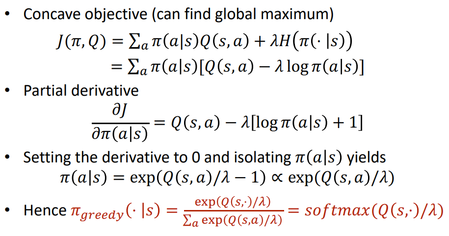
Concave objective (can find global maximum):
Take partial derivative w.t.r. to the action probability:

Set derivative to 0 and find maximum:

The only problem \(\pi(a|s)\) is a probability distribution:

Policy Improvement: Proof
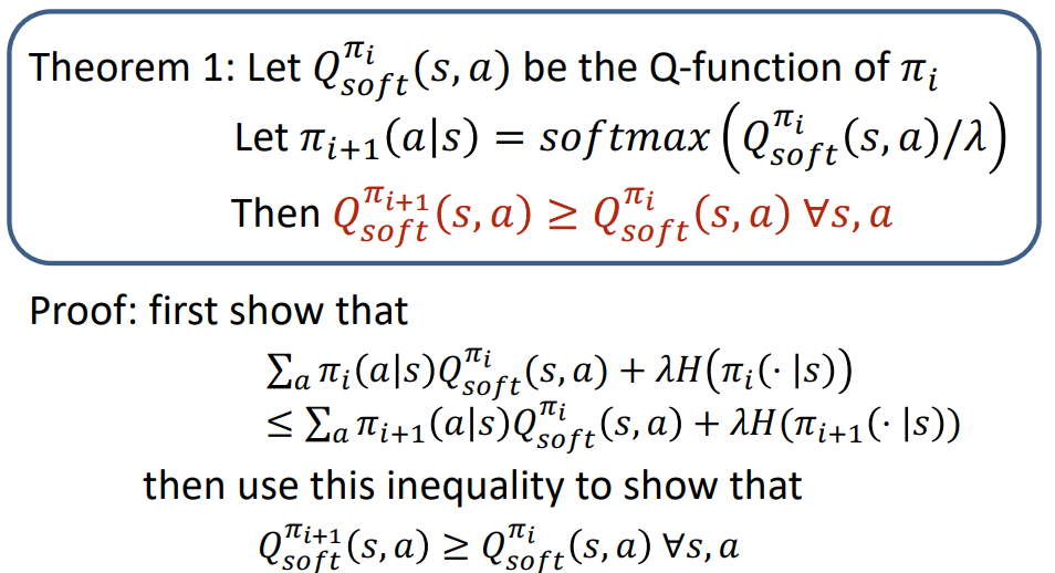
Policy Improvement: Proof
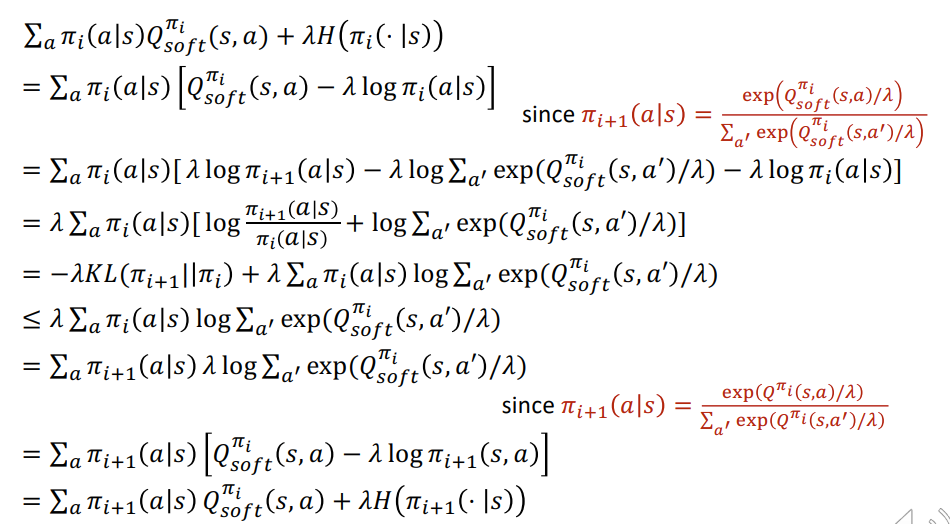
Policy Improvement: Proof
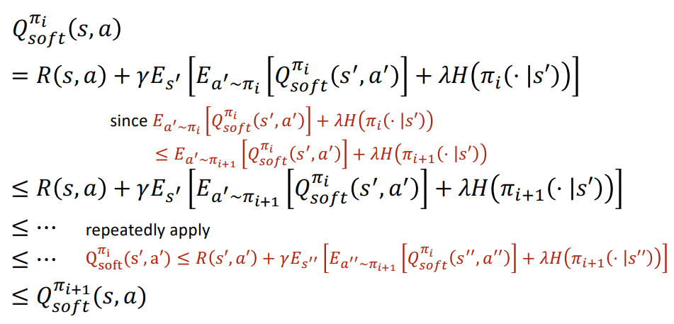
Soft-Actor Critic
Policy Evaluation doesn't need to change:
Lets upgrade Soft Policy iteration for continuous action space!

Policy Improvement step for continuous policy:


Soft-Actor Critic
Critic approximate Policy Evaluation. Trains with MSE:
Actor apporximate Policy Improvement. Trains with the following loss:
where:
SAC evolution:

Soft-Actor Critic
Implementation Details:
- Reparametrization trick for policy:
- Therefore actor loss becomes:
- Twin Critics for Q-value (like in TD3)
- Moving average update for targets (like in TD3, DDPG)
- tanh squashing for outputs: \(a_t = tanh(f_{\phi}(\epsilon_t; s_t)) \)


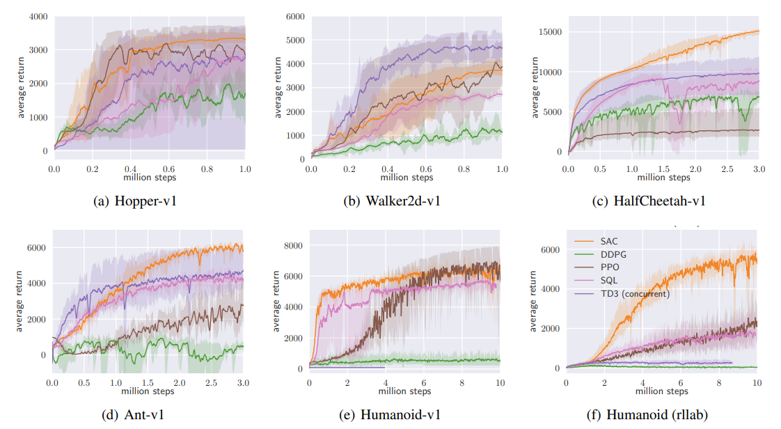
Soft-Actor Critic: Results
Conclusion:
For environments with continual action spaces start from either TD3 or SAC


TD3 graph: TD3 > SAC
SAC graph: SAC > TD3