Non-Euclidean Motion Planning with Graphs of Geodesically-Convex Sets

Thomas Cohn

November 18, 2022
(Broad) Outline
- Motivation
- A Roboticist's Intro to Differential Geometry
- Motion Planning in Non-Euclidean Spaces
Part 1
Motivation
Motion Planning with GCS
- Represent C-Free with convex sets
- Formulate shortest path problem as MICP
- Can solve to optimality (branch and bound)
- In practice, relax and round yields a good result
Shortest Paths in Graphs of Convex Sets, Marcucci et. al.
Motion Planning around Convex Obstacles with Convex Optimization, Marcucci et. al.
What about non-Eucldiean configuration spaces?
What Is a Non-Euclidean Configuration Space?
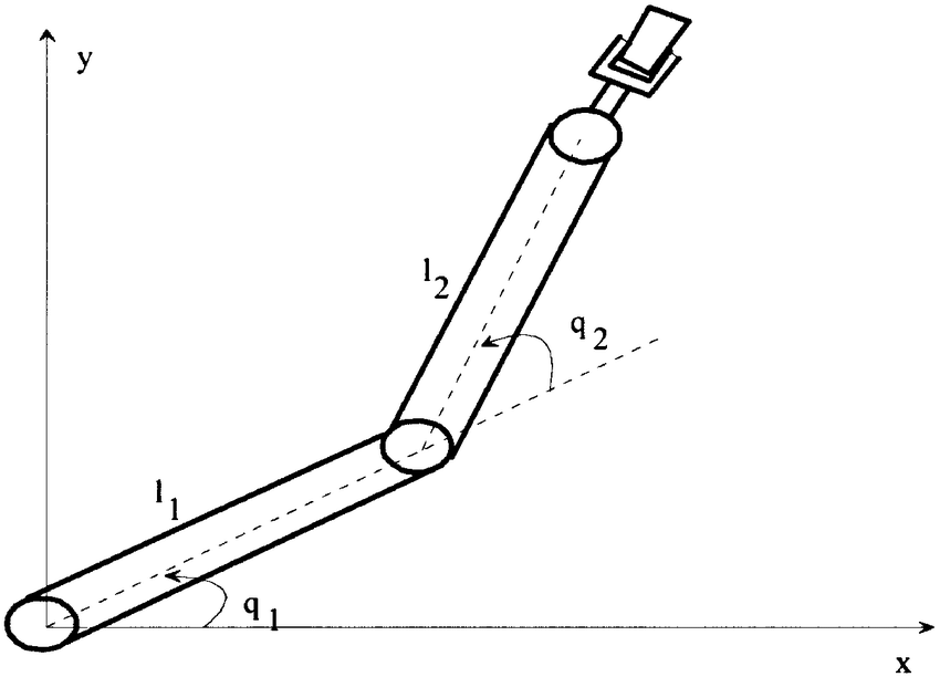
Robust Combined Adaptive and Variable Structure Adaptive Control of Robot Manipulators, Yu
(No joint limits)
"Locally" Euclidean Spaces

?
?
?
?
Manifolds
?
?
?
?
Part 2
A Roboticist's Intro to Differential Geometry
Enter: Manifolds
A manifold is a locally-Euclidean topological space
- Topological Manifolds
- Smooth Manifolds
- Riemannian Manifolds
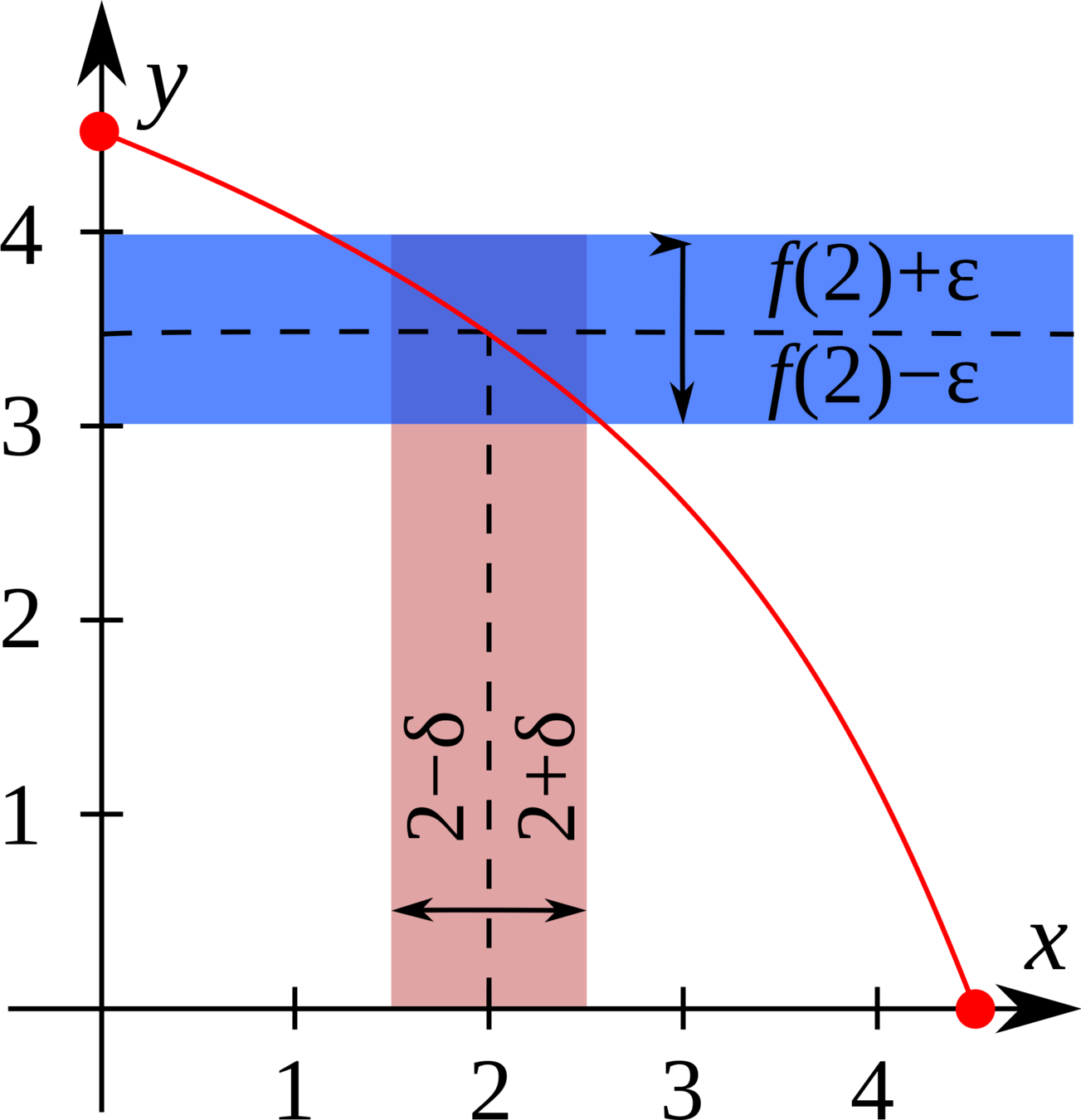
Continuity (Intuition)
Continuous functions take nearby points to nearby points
What is a Topological Space?
A rule for which functions are continuous by defining what "nearby" means
Explicitly: a rule for constructing arbitrarily small* neighborhoods around points
Examples:
(Path) Connectedness
A topological space is path connected if there is a continuous curve joining any two points.
A continuous curve is the image of a function \(f:[0,1]\to X\)
Compactness
A set is compact if every open cover has a finite subcover
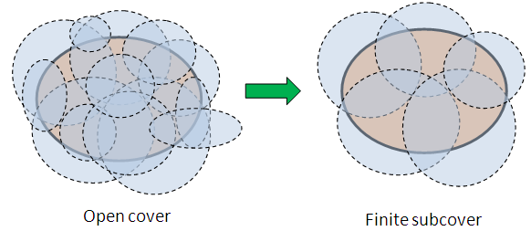
Heine-Borel Theorem: In Euclidean spaces, compact iff closed and bounded
Extreme Value Theorem: Functions over compact sets have max and min values (useful for optimization theory)
Summary
-
Continuity
- Does a function map nearby points to nearby points?
-
Path-Connectedness
- Can one "move" between two points?
-
Compactness
- Do functions have extrema?
Definition of a Manifold
A manifold is a locally-Euclidean topological space
Definition of a Manifold
A manifold is a locally-Euclidean topological space
Introduction to Smooth Manifolds, Lee
Definition of a Manifold
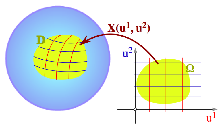
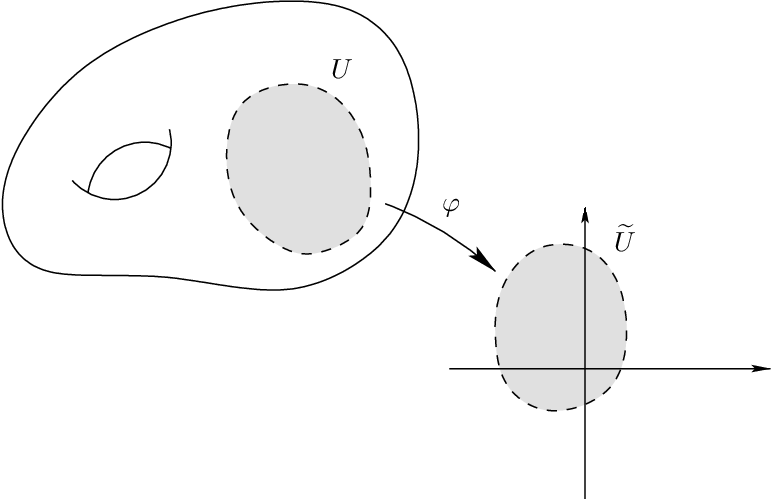
Locally-Euclidean: any \(x\in\mathcal{M}\) is contained in an open set \(U\subseteq\mathcal{M}\) such that \(U\) is homeomorphic to a subset of Euclidean space
Introduction to Smooth Manifolds, Lee
A manifold is a locally-Euclidean topological space
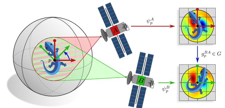
Charts and Atlases
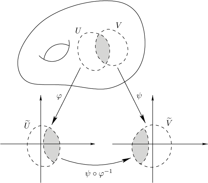
Coordinate chart: An open set (sufficiently small neighborhood) \(U\subseteq\mathcal{M}\) with a homeomorphism \(\psi\)
Atlas: A collection of charts that cover \(\mathcal{M}\)
Transition Map: How to move from one chart to another
Introduction to Smooth Manifolds, Lee
Smooth Manifolds
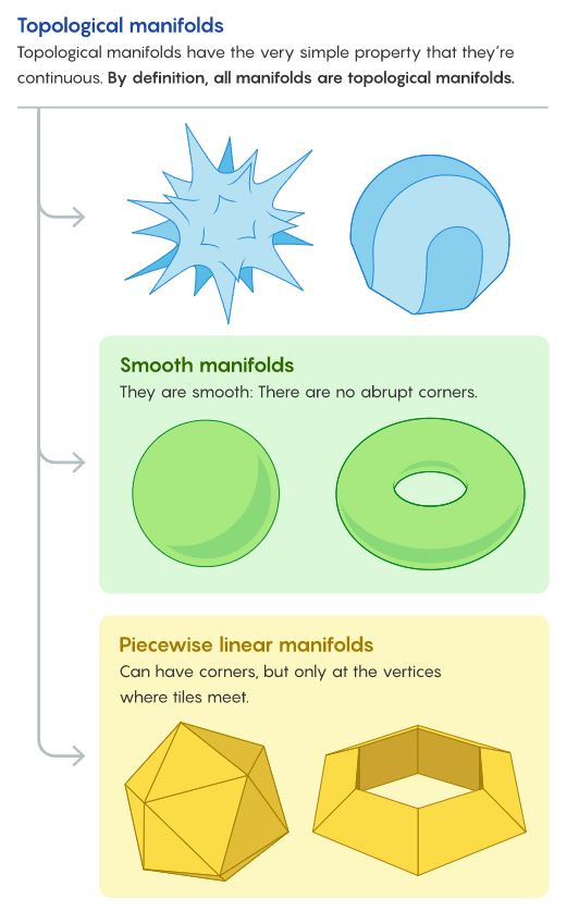
A manifold is smooth if its atlas has smooth transition maps
Intuition: no corners or edges
Can have different levels of smoothness (\(n\)-times continuously-differentiable vs analytic)
Derivatives and Integrals
We can compute directional derivatives for functions
We can take integrals of functions, vector fields, etc.
Interesting, but not relevant for the current project
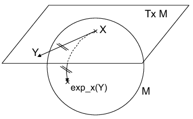
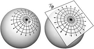
The Tangent Space

Given a point \(x\in M\), we can consider the velocity of curves that pass through \(x\)
This forms a vector space \(T_xM\), called the tangent space
Maps Between Manifolds
Let \(M\) and \(N\) be two manifolds, and \(\phi:M\to N\) a smooth function
We can use \(\phi\) to "move information" between \(M\) and \(N\)
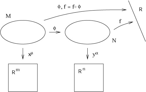
Pushforward
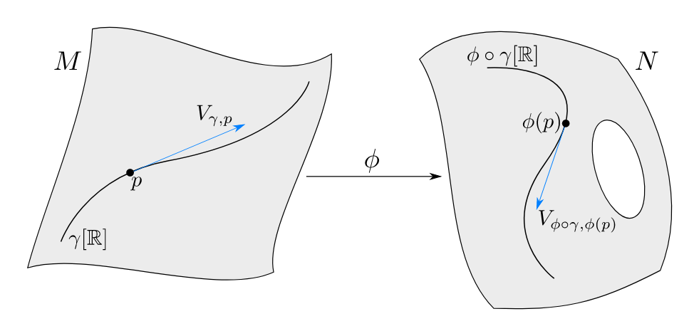
The pushforward \(d\phi\) moves tangent vectors from \(M\) to \(N\)
Pullback
The pullback \(\phi^*\) moves functions from \(N\) to \(M\)
\(\phi^*f=f\circ\phi\)
Application: RMPs
Riemannian Motion Policies use pushforwards and pullbacks to unify controllers across different configuration spaces
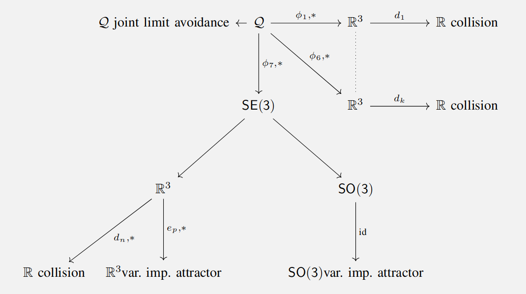
RMPs for Safe Impedance Control in Contact-Rich Maniuplation, Shaw et. al.
Product Manifolds
The Cartesian product of two manifolds is itself a manifold
Lie Groups
What if a manifold is also a group?
Need the group operation and inversion to be smooth maps
Examples: SO(3), SE(3)
Coordiante Independent Convolutional Networks -- Isometry and Gauge Equivariant Convolutions on Riemannian Manifolds, Weiler et. al.
Riemannian Manifolds

Motivation: Distance
Arc length depends on the parameterization of the charts
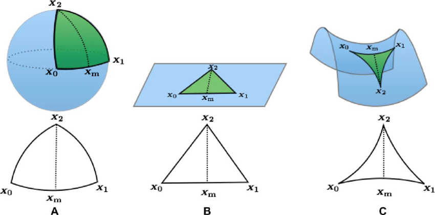
Motivation: Curvature
Triangles and angles look different
Riemannian Metric
A Riemannian Metric assigns an inner product to each tangent space
The inner product must be a positive definite bilinear form, and it must vary smoothly along the manifold
Allows us to define curvature, and compute distances
Curvature
- Describes how the local geometry differs from Euclidean
- Explicitly, a fourth-order tensor (with complex symmetries)
- Intuition: what do angles and triangles look like?
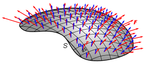
Arc Length
Consider a piecewise-differentiable curve \(\gamma\in\mathcal{C}^{1}_{\operatorname{pw}}([a,b],\mathcal{M})\)
Its arc length is \(\displaystyle L(\gamma)=\int_a^b \sqrt{\left<\gamma'(s),\gamma'(s)\right>^{\mathcal{M}}_{\gamma(s)}}\,ds\)
For any two points \(p,q\in\mathcal{M}\), the distance between them is defined to be
\[\inf\{L(\gamma)\,|\,\gamma\in\mathcal{C}^{1}_{\operatorname{pw}}([0,1],\mathcal{M}),\gamma(0)=p,\gamma(1)=q\}\]
This integral is parameterization-independent
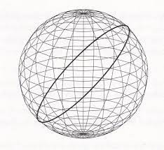
Geodesics
A geodesic is a (locally) length-minimizing curve -- solution to
\[\operatorname{arg}\,\inf\{L(\gamma)\,|\,\gamma\in\mathcal{C}^{1}_{\operatorname{pw}}([0,1],\mathcal{M}),\gamma(0)=p,\gamma(1)=q\}\]
Variational calculus problem -- solution satisfies Euler-Lagrange system of differential equations
As a result, each geodesic is uniquely defined by its initial conditions
Computation: forward integrate the differential equations
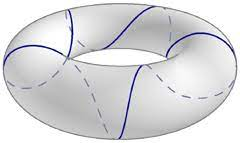
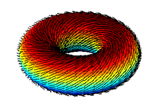
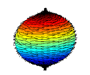
Examples of Geodesics
Exponential Map
Recall: tangent vectors are velocities of curves through a point
Exponential map intuition:
- Can extend a tangent vector to a geodesic
- Length of the vector corresponds to distance along the geodesic
- Yields a coordinate chart, called the "normal" coordinates
Part 3
Motion Planning in Non-Euclidean Spaces
Problem Statement
Configuration space \(\mathcal{Q}\) as a Riemannian manifold
\(\mathcal{M}\subseteq\mathcal{Q}\) is the set of collision free configurations, \(\bar{\mathcal{M}}\) its closure
The shortest path between \(p,q\in\bar{\mathcal{M}}\) is the solution to the optimization problem
\[\begin{array}{rl} \argmin & L(\gamma)\\ \textrm{subject to} & \gamma\in\mathcal{C}^{1}_{\operatorname{pw}}([0,1],\bar{\mathcal{M}})\\ & \gamma(0)=p\\ & \gamma(1)=q\end{array}\]
The Plan...
- Formulate GCS on a Manifold
- Add Structure to the Problem
- Transform to GCS in Euclidean Space
Geodesic Convexity
- Bring the ideas of convexity to Riemannian manifolds
- Enables optimization with strong guarantees
- Young but growing area of study
Re-visiting Riemannian geometry of symmetric positive definite matrices for the analysis of functional connectivity, You et. al.
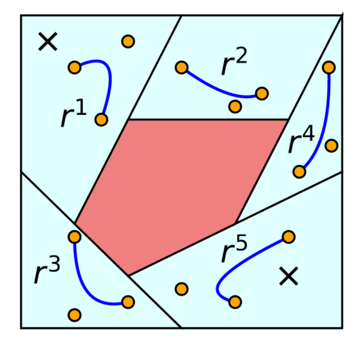
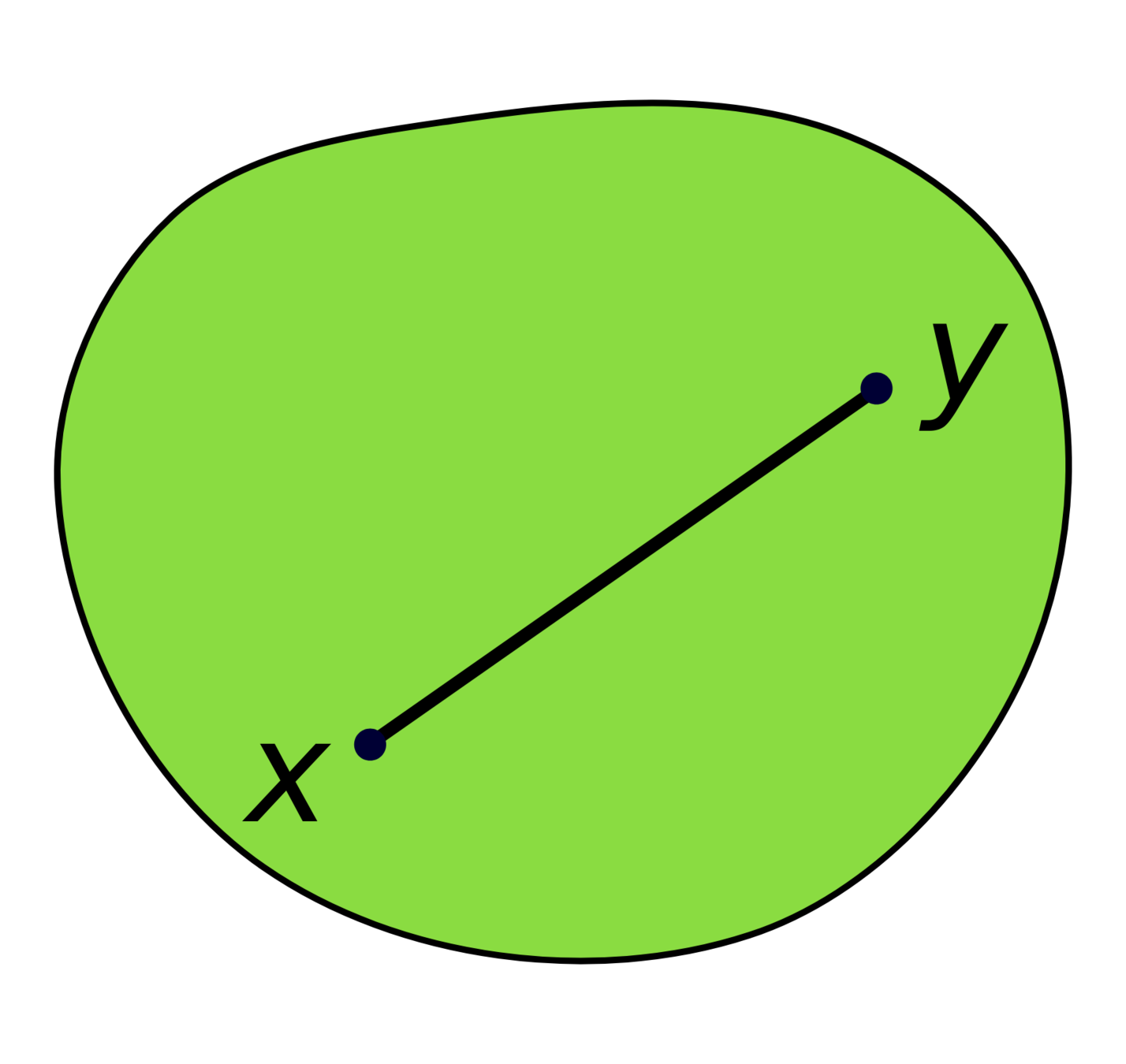
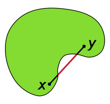
Convex Sets
A set \(X\subseteq\mathbb{R}^n\) is convex if \(\forall p,q\in X\), the line connecting \(p\) and \(q\) is contained in \(X\)
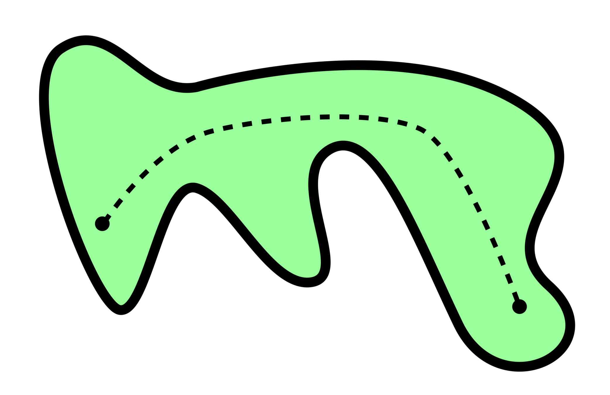
Geodesically Convex Sets
A set \(X\subseteq\mathcal{M}\) is strongly geodesically convex if \(\forall p,q\in X\), there is a unique length-minimizing geodesic (w.r.t. \(\mathcal{M}\)) connecting \(p\) and \(q\), which is completely contained in \(X\).
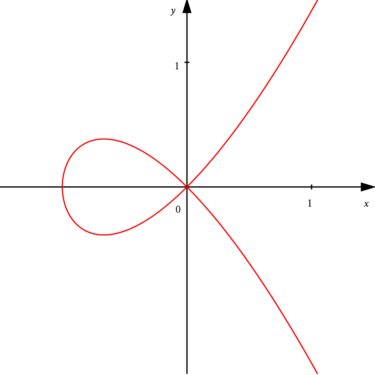
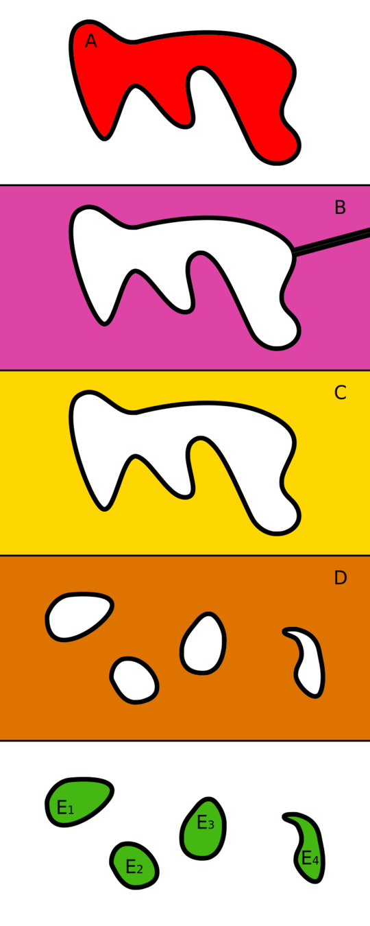
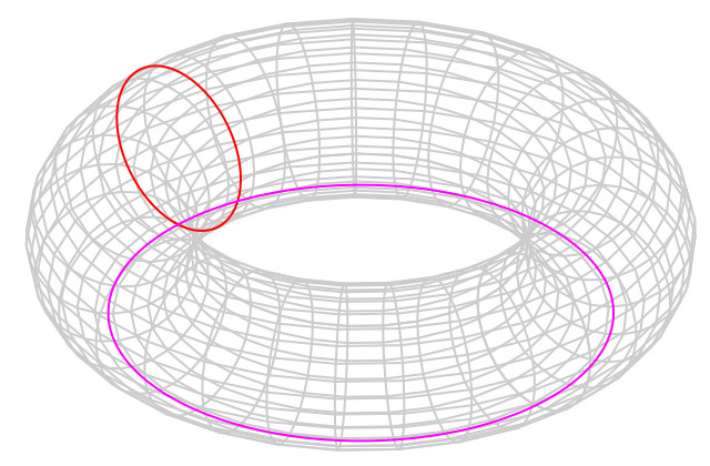
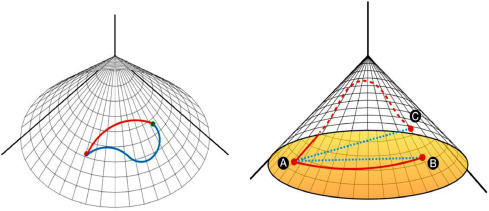
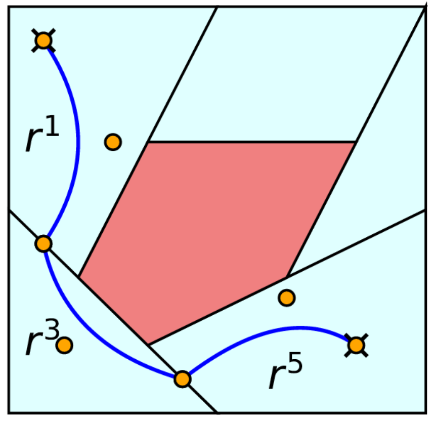
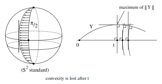
Some Sets Look Convex
(But Aren't)
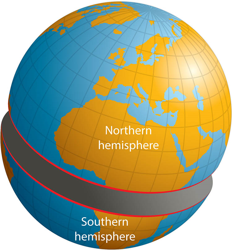
Sets can be convex in local coordinates, but not geodesically-convex on the manifold
Geodesics can go "the wrong way around"
Radius of convexity: how large can a set be and still be convex?
Convex Functions
A function \(f:X\to\mathbb{R}\) is convex if for any \(x,y\in X\) and \(\lambda\in[0,1]\), we have
\(f(\lambda x+(1-\lambda)y)\le\)
\(\lambda f(x)+(1-\lambda) f(y)\)
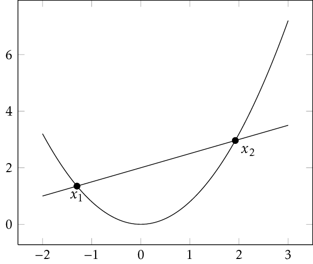
Geodesically Convex Functions
A function \(f:\mathcal{M}\to\mathbb{R}\) is geodesically convex if for any \(x,y\in \mathcal{M}\) and any geodesic \(\gamma:[0,1]\to\mathcal{M}\) such that \(\gamma(0)=x\) and \(\gamma(1)=y\), \(f\circ\gamma\) is convex
Convex Functions
Geodesically Convex Functions

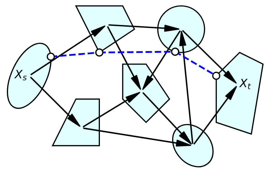
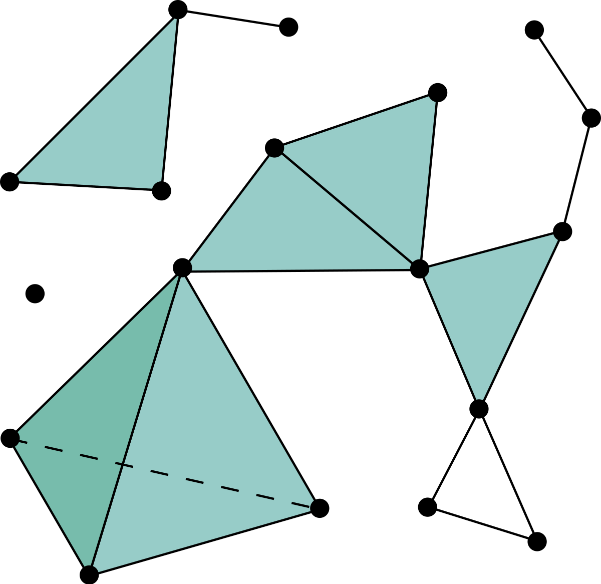
A Graph of Geodesically Convex Sets (GGCS)
A directed graph \(G=(V,E)\)
- For each vertex \(v\in V\), there is a strongly geodesically convex manifold \(\mathcal{Y}_v\)
- For each edge \(e=(u,v)\in E\), there is a cost function \(\ell_e^\mathcal{Y}:\mathcal{Y}_u\times\mathcal{Y}_v\to\mathbb{R}\)
- \(\ell_e^\mathcal{Y}\) must be geodesically convex with respect to the product metric on \(\mathcal{Y}_u\times\mathcal{Y}_v\)
GCS

GGCS

Shortest Paths in GGCS
Mixed-Integer Riemannian Optimization? No existing literature.
Better option: transform into a GCS problem
Pullback of Sets and Edges

Shortest Paths in GGCS
For each \(v\in V\), let \(\psi_v:\mathcal{Y}_v\to\mathbb{R}^n\) be a coordinate chart
Define \(X_v=\psi_v(\mathcal{Y}_v)\)
For each \(e=(u,v)\in E\), new edge cost:
\[\ell_e(x_u,x_v)=\ell_e^\mathcal{Y}(\psi_u^{-1}(x_u),\psi_v^{-1}(x_v))\]
If all \(X_v\) and \(\ell_e\) are convex, we have a valid GCS problem
Mixed-Integer Riemannian Optimization? No existing literature.
Better option: transform into a GCS problem
Problem Statement
Configuration space \(\mathcal{Q}\) as a Riemannian manifold
\(\mathcal{M}\subseteq\mathcal{Q}\) is the set of collision free configurations, \(\bar{\mathcal{M}}\) its closure
The shortest path between \(p,q\in\bar{\mathcal{M}}\) is the solution to the optimization problem
\[\begin{array}{rl} \argmin & L(\gamma)\\ \textrm{subject to} & \gamma\in\mathcal{C}^{1}_{\operatorname{pw}}([0,1],\bar{\mathcal{M}})\\ & \gamma(0)=p\\ & \gamma(1)=q\end{array}\]
Additional Requirements
\(\mathcal{Q}\) is zero-curvature
- Negative-curvature manifolds not common in robotics
- Distance metric on positive curvatures is nonconvex 😡
Zero-Curvature is Still Useful
- All 1-dimensional manifolds
- Continuous revolute joints
- \(\operatorname{SO}(2)\), \(\operatorname{SE}(2)\)
- Products of flat manifolds
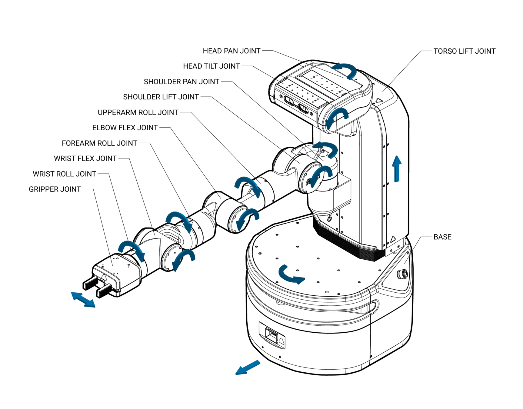
Fetch Robot Configuration
Space: \(\operatorname{SE}(2)\times \mathbb{T}^3\times \mathbb{R}^7\)
Additional Requirements
\(\mathcal{Q}\) is zero-curvature
- Negative-curvature manifolds not common in robotics
- Distance metric on positive curvatures is nonconvex
\(\mathcal{A}=\{(X_v,\psi_v)\}_{v\in V}\) is a finite atlas of \(\mathcal{M}\), with each \(X_v\) strongly geodesically convex, and each \(\psi_v\) an isometry
- Necessary for computation
- Leads to nice theoretical results
Reminder: Transition Maps
How to move from one chart to another
Introduction to Smooth Manifolds, Lee
Reformulating as GCS
Decision variables:
\(\forall v\in V\), we have \(x_v=(x_{v,0},x_{v,1})\in\psi_v(X_v)^2\)
Edge costs:
\[\ell_e(x_u,x_v)=||x_{u,0}-x_{u,1}||_2,\quad\forall e=(u,v)\in E\]
Edge constraints:
\[\tau_{u,v}(x_{u,1})=x_{v,0},\quad\forall e=(u,v)\in E\]
(\(\tau_{u,v}\) is the transition map from \(X_u\) to \(X_v\))
Motion Planning around Obstacles with Convex Optimization, Marcucci et. al.
Why Transition Maps?
Want all equations to live in Euclidean coordinates
Equivalent conditions:
\[\psi_u^{-1}(x_{u,1})=\psi_v^{-1}(x_{v,0})\;\;\Leftrightarrow\;\;\tau_{u,v}(x_{u,1})=x_{v,0}\]
Motion Planning around Obstacles with Convex Optimization, Marcucci et. al.
Nice Theoretical Results?
- There is a shortest path \(\gamma\) connecting \(p\) to \(q\) through \(\bar{\mathcal{M}}\) such that
- \(\gamma\) is piecewise geodesic
- Each geodesic segment is contained in some \(\bar{X}_u\)
- \(\gamma\) passes through each \(\bar{X}_u\) at most once
-
Ensures that a shortest path is feasible for GGCS
- Transition maps are affine functions (in particular, they are an orthogonal transformation plus a translation)
- Formal equivalence of GGCS and transformed GCS problem
Results
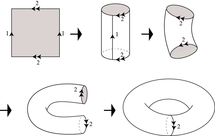
"Asteroids" World
Square with opposite edges identified
Configuration Space: \(\mathbb{T}^2\)
Planar Arm
A robot arm with 5 continuous revolute joints in the plane
Configuration Space: \(\mathbb{T}^5\)
(No self collisions)

(Modified) Kuka iiwa Arm
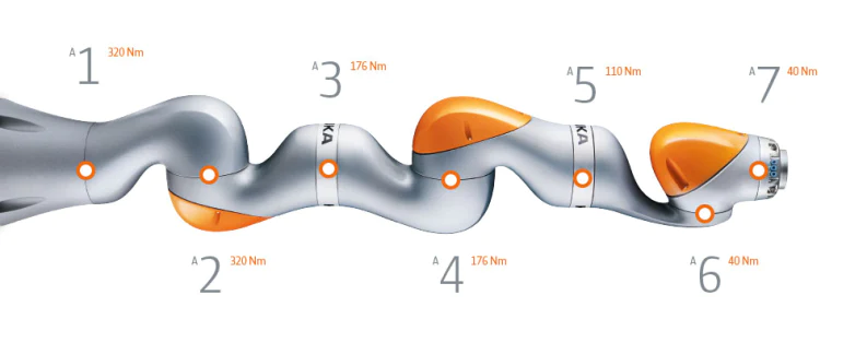
Modified to be a continuous revolute joint
Practicum
Generating Atlases
Key idea: generate within a chart in the first place
Use IRIS in configuration space, add bounds on the diameter of the set to preserve strong convexity
A Panoramic View of Riemannian Geometry, Berger
Further Motion Planning
All Bézier curve constructions also hold on the manifold
For higher-order continuity constraints, want tangent vectors to be equal. Use the pushforward!
Higher Order Continuity
Order \(0\) continuity, order \(k\) splines:
\[\tau_{u,v}(x_{u,k})=x_{v,0}\quad\forall e=(u,v)\in E\]
Order \(m\) continuity, order \(k\) splines:
\[(\tau_{u,v})_*(x^{(m)}_{u,k})=x^{(m)}_{v,0}\quad\forall e=(u,v)\in E\]
If \(\tau_{u,v}\) is an isometry, then \(\tau_{u,v}(x)=R(x)+T(x)\) for \(R\in\operatorname{O}(n)\) and \(T\in\operatorname{E}(n)\). Thus, \((\tau_{u,v})_*=R\).
Globally-Aligned Coordinates
In some (most?) cases, we can align the coordinate systems
If so, we have \(\tau_{u,v}\in \operatorname{T}(n)\) and \((\tau_{u,v})_*=I_n\), \(\forall e=(u,v)\in E\)
Non-Euclidean Motion Planning with Graphs of Geodesically-Convex Sets
Thomas Cohn
November 18, 2022