Motion Planning in Minimal Coordinates for Kinematically-Constrained Systems
Thomas Cohn
September 23, 2026
Presentation for the MIT REx Lab group meeting


Robot Locomotion Group
Which Kinematically-Constrained Systems?
Motion Planning in Minimal Coordinates for Kinematically-Constrained Systems
Thomas Cohn, Robot Locomotion Group, MIT CSAIL
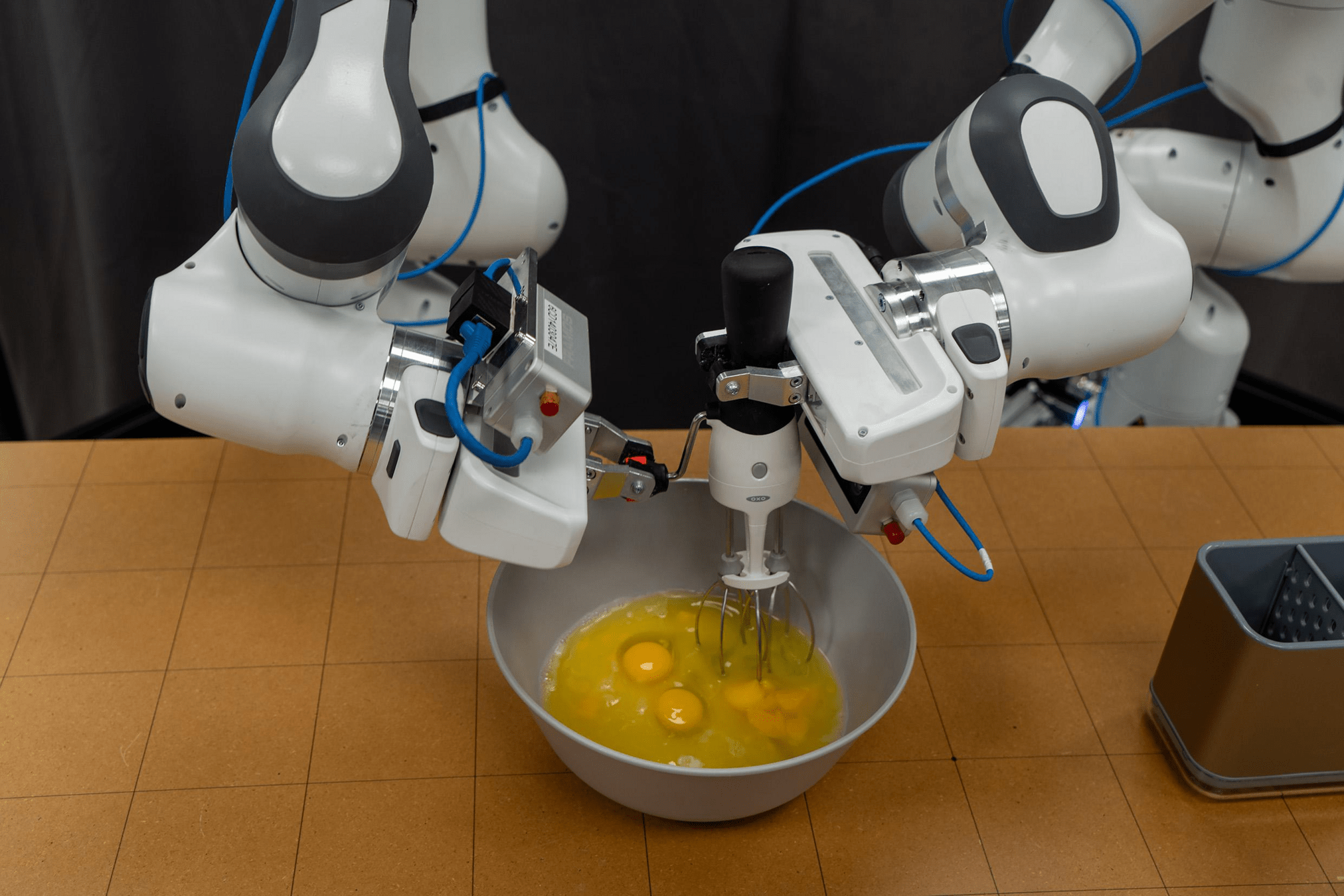
Toyota Research Institute
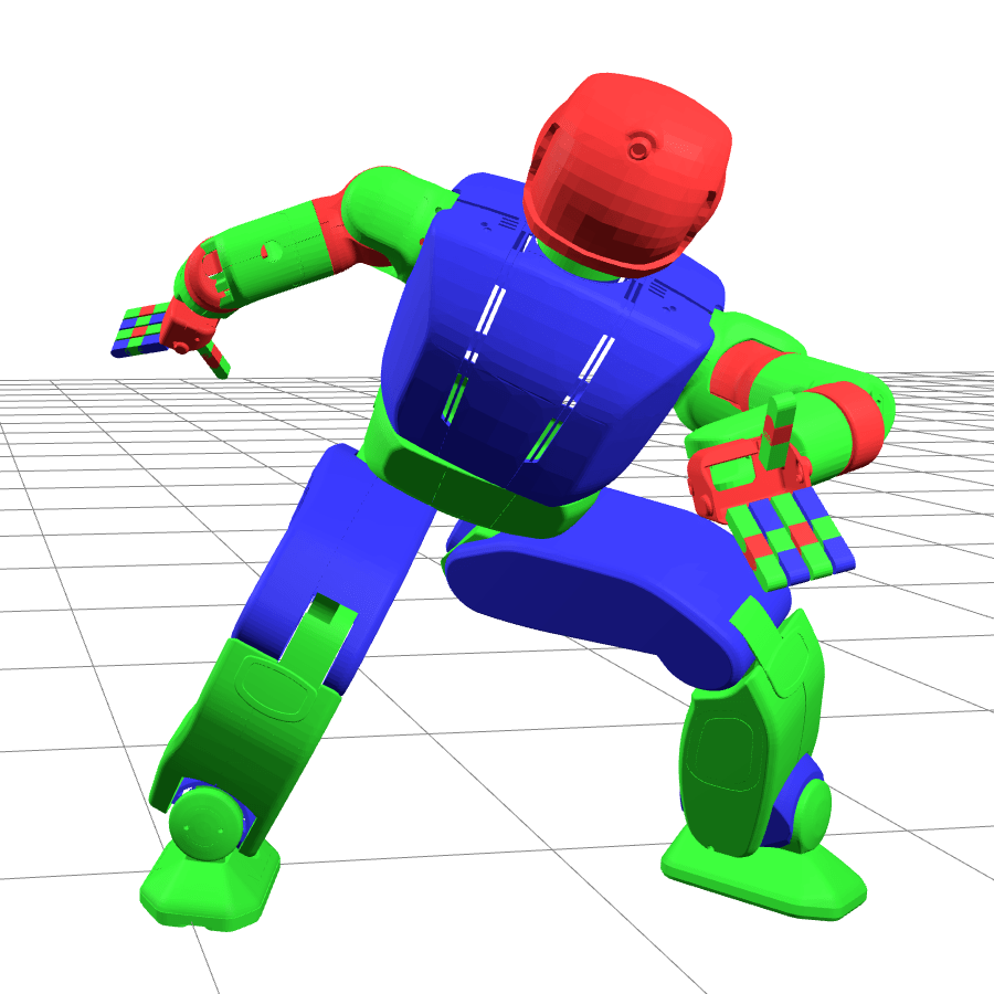
Boston Dynamics
The Configuration-Space Picture
Motion Planning in Minimal Coordinates for Kinematically-Constrained Systems
Learning the Metric of Task Constraint Manifolds for Constrained Motion Planning, Zha et al. 2018
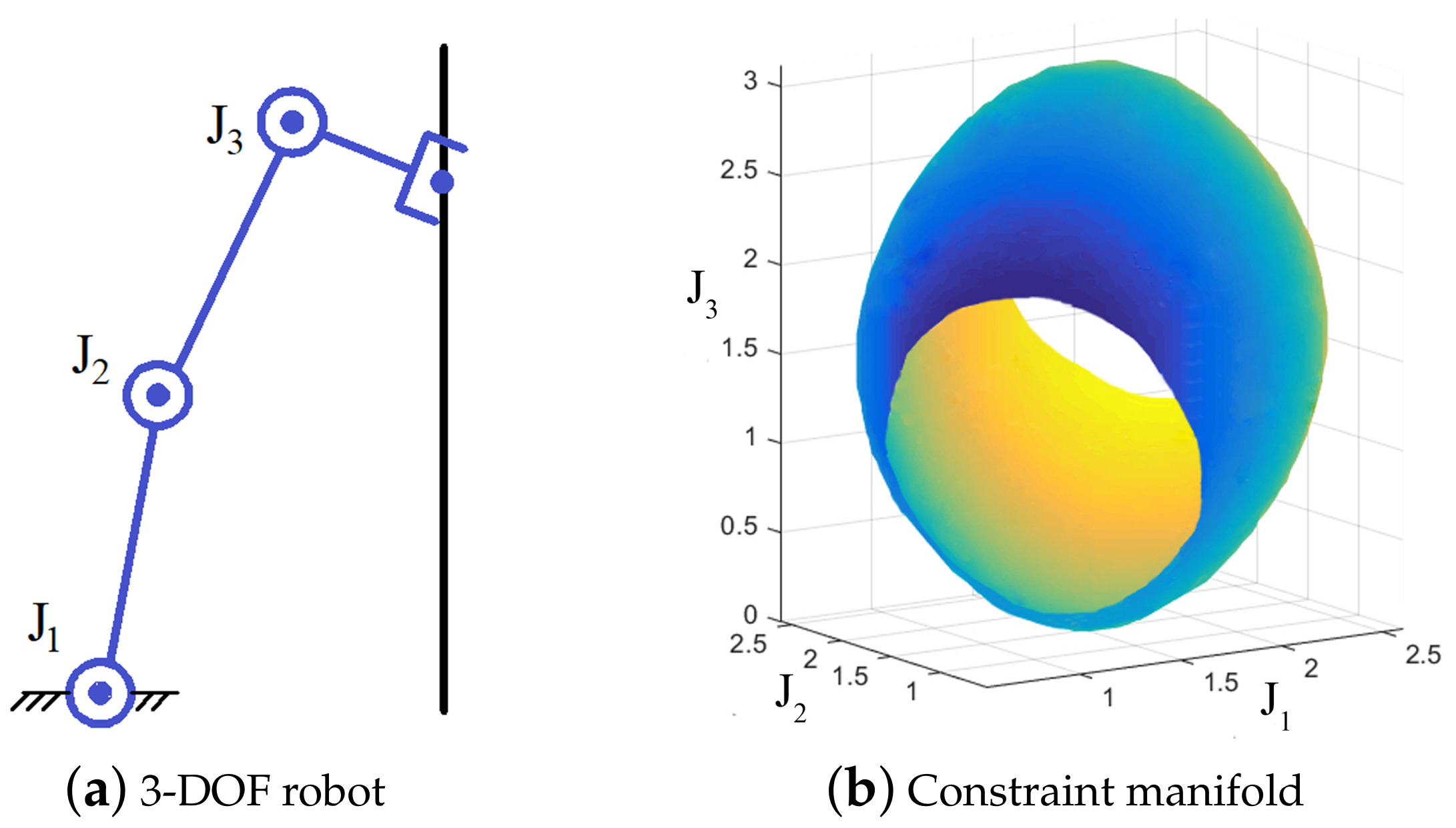
Thomas Cohn, Robot Locomotion Group, MIT CSAIL
The Predominant, "Extrinsic" Approach
Motion Planning in Minimal Coordinates for Kinematically-Constrained Systems
Sampling-Based Methods for Motion Planning with Constraints, Kingston et al. 2018
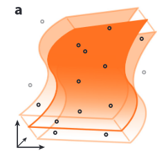
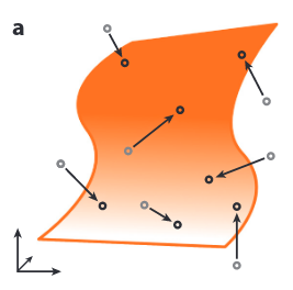
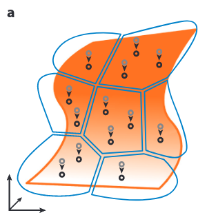
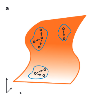
Sampling-Based Planners
Trajectory Optimizers
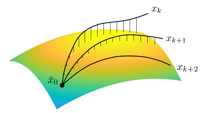
Trajectory Optimization on Manifolds: A Theoretically-Guaranteed Embedded Sequential Convex Programming Approach, Bonalli et al. 2019
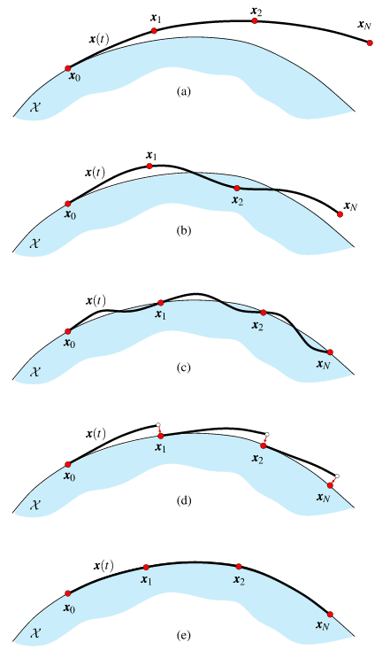
Direct Collocation Methods for Trajectory Optimization in Constrained Robotic Systems, Bordalba et al. 2022
Thomas Cohn, Robot Locomotion Group, MIT CSAIL
An "Intrinsic" Alternative?
Motion Planning in Minimal Coordinates for Kinematically-Constrained Systems
Thomas Cohn, Robot Locomotion Group, MIT CSAIL
"Would be great if we could do it, but difficult or impossible in practice"
Paraphrased from the textbooks of LaValle, Latombe, Siciliano and Khatib, Lynch and Park.
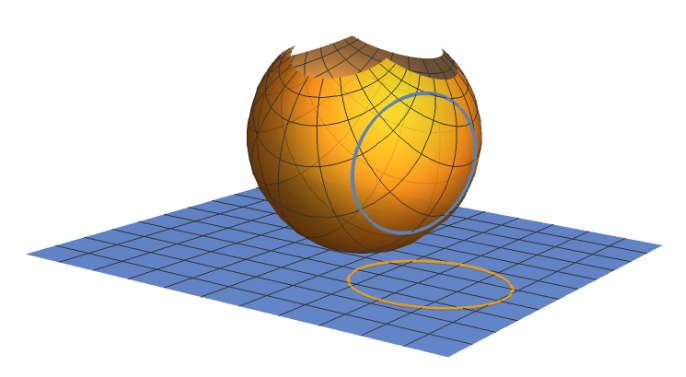
Trajectory Optimization On Manifolds with
Applications to \(SO(3)\) and \(\mathbb{R}^3 \times S^2\), Watterson et al. 2018
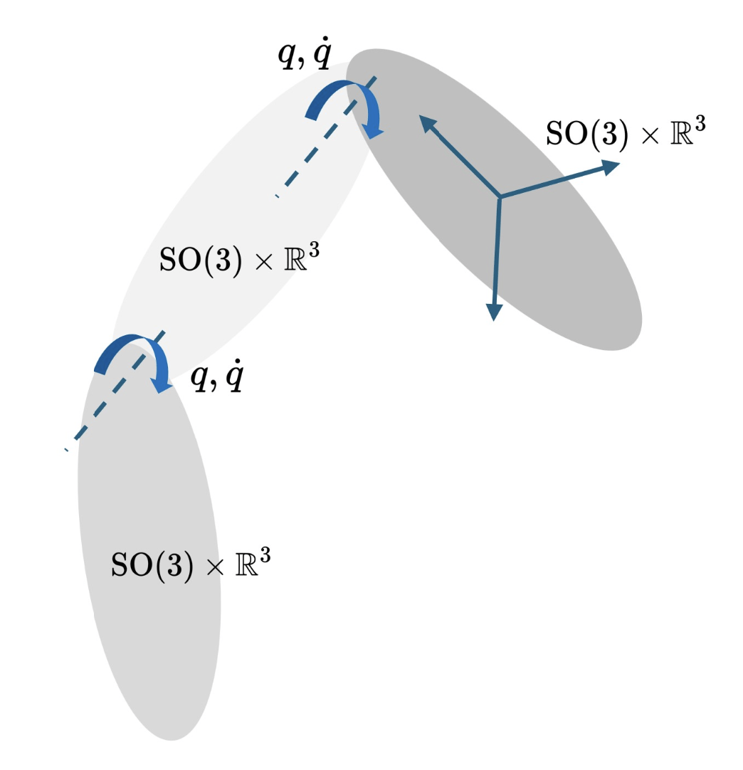
Riemannian Direct Trajectory Optimization of Rigid Bodies on Matrix Lie Groups, Teng et al. 2025
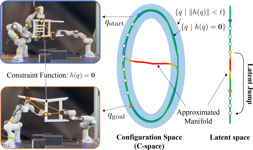
A Constrained Motion Planning Method Exploiting Learned Latent Space for High-Dimensional State and Constraint Spaces, Park et al. 2024
- Planning with Parameterizations
- Change of Variables with Analytic IK
- Resolving the "many-to-one" problem
- Reachability constraints: describing the domain
- Gradients through IK Solvers (without Introspection)
- The inverse function theorem
- Domain extensions and boundary reachability
- The Benchmark Suite: Where the Solvers Struggle
- Next Steps: a Trust-Region Solver?
Outline for the Remainder of the Talk
Motion Planning in Minimal Coordinates for Kinematically-Constrained Systems
Thomas Cohn, Robot Locomotion Group, MIT CSAIL
Collision-Free Motion Planning Problem:
\[\begin{array}{rl}\min_\gamma & L(\gamma)\\ \operatorname{s.t.} & \gamma:[0,1]\to\mathbb R^n\\ & \gamma(0)=q_0,\gamma(1)=q_1\\ & g(\gamma(t))\le 0,\forall t\in[0,1]\end{array}\]
Constrained Collision-Free Motion Planning Problem:
\[\begin{array}{rl}\min_\gamma & L(\gamma)\\ \operatorname{s.t.} & \gamma:[0,1]\to\mathbb R^n\\ & \gamma(0)=q_0,\gamma(1)=q_1\\ & g(\gamma(t))\le 0,\forall t\in[0,1]\\ & h(\gamma(t))=0,\forall t\in[0,1]\end{array}\]
The Constrained Planning Problem
Thomas Cohn, Robot Locomotion Group, MIT CSAIL
Motion Planning in Minimal Coordinates for Kinematically-Constrained Systems
Constrained Collision-Free Motion Planning Problem:
\[\begin{array}{rl}\min_\gamma & L(\gamma)\\ \operatorname{s.t.} & \gamma:[0,1]\to\mathbb R^n\\ & \gamma(0)=q_0,\gamma(1)=q_1\\ & g(\gamma(t))\le 0,\forall t\in[0,1]\\ & h(\gamma(t))=0,\forall t\in[0,1]\end{array}\]
- Constraint manifold \(\mathcal M=\{q\in\mathbb R^n:h(q)=0\}\)
- Parameterization \(\phi:\mathbb R^m\to\mathbb R^n\), reachable domain \(\mathcal V\subseteq\mathbb R^m\)
- Require:
- \(\phi(\mathcal V)\subseteq\mathcal M\)
- \(\phi\) is differentiable almost everywhere
Assume a Parameterization
Thomas Cohn, Robot Locomotion Group, MIT CSAIL
Motion Planning in Minimal Coordinates for Kinematically-Constrained Systems
\[\begin{array}{rl}\min_\gamma & L(\gamma)\\ \operatorname{s.t.} & \gamma:[0,1]\to\mathbb R^n\\ & \gamma(0)=q_0,\gamma(1)=q_1\\ & g(\gamma(t))\le 0,\forall t\in[0,1]\\ & h(\gamma(t))=0,\forall t\in[0,1]\end{array}\]
- Constraint manifold \(\mathcal M=\{q\in\mathbb R^n:h(q)=0\}\)
- Parameterization \(\phi:\mathbb R^m\to\mathbb R^n\), reachable domain \(\mathcal V\subseteq\mathbb R^m\)
- Require:
- \(\phi(\mathcal V)\subseteq\mathcal M\)
- \(\phi\) is differentiable almost everywhere
\[\begin{array}{rl}\min_{\tilde\gamma}& L(\phi\circ\tilde\gamma)\\ \operatorname{s.t.} & \tilde\gamma:[0,1]\to\mathcal V\\ & \tilde\gamma(0)=\tilde q_0,\tilde\gamma(1)=\tilde q_1\\ & g((\phi\circ\tilde\gamma)(t))\le 0,\forall t\in[0,1]\\ & h((\phi\circ\tilde\gamma)(t))=0,\forall t\in[0,1]\end{array}\]
The Parameterized Planning Problem
Thomas Cohn, Robot Locomotion Group, MIT CSAIL
Motion Planning in Minimal Coordinates for Kinematically-Constrained Systems
\[\begin{array}{rl}\min_{\tilde\gamma}& L(\phi\circ\tilde\gamma)\\ \operatorname{s.t.} & \tilde\gamma:[0,1]\to\mathcal V\\ & \tilde\gamma(0)=\tilde q_0,\tilde\gamma(1)=\tilde q_1\\ & g((\phi\circ\tilde\gamma)(t))\le 0,\forall t\in[0,1]\\ & h((\phi\circ\tilde\gamma)(t))=0,\forall t\in[0,1]\end{array}\]
"Reachability Constraint"
Assume we can construct \(\tilde q_i\) such that \(\phi(\tilde q_i)=q_i\), \(i\in\{0,1\}\).
Becomes more Complicated
Eliminated by Construction: \(\tilde\gamma(t)\in\mathcal V\Rightarrow h((\phi\circ\tilde\gamma)(t))=0\)
The Parameterized Planning Problem
Thomas Cohn, Robot Locomotion Group, MIT CSAIL
Motion Planning in Minimal Coordinates for Kinematically-Constrained Systems
Planning Examples
Thomas Cohn, Robot Locomotion Group, MIT CSAIL
Motion Planning in Minimal Coordinates for Kinematically-Constrained Systems
Trajectory Optimization
Sampling-Based Planning
Graphs of Convex Sets
Parameterizing Kinematic Graphs
Motion Planning in Minimal Coordinates for Kinematically-Constrained Systems
Thomas Cohn, Robot Locomotion Group, MIT CSAIL
Key idea (Han and Amato 2001; Xie and Amato 2004):
- Split into active and passive chains
- Specify active chains as input
- Solve for passive chains with IK
Parameterizing Kinematic Graphs
Motion Planning in Minimal Coordinates for Kinematically-Constrained Systems
Thomas Cohn, Robot Locomotion Group, MIT CSAIL
Key idea (Han and Amato 2001; Xie and Amato 2004):
- Split into active and passive chains
- Specify active chains as input
- Solve for passive chains with IK
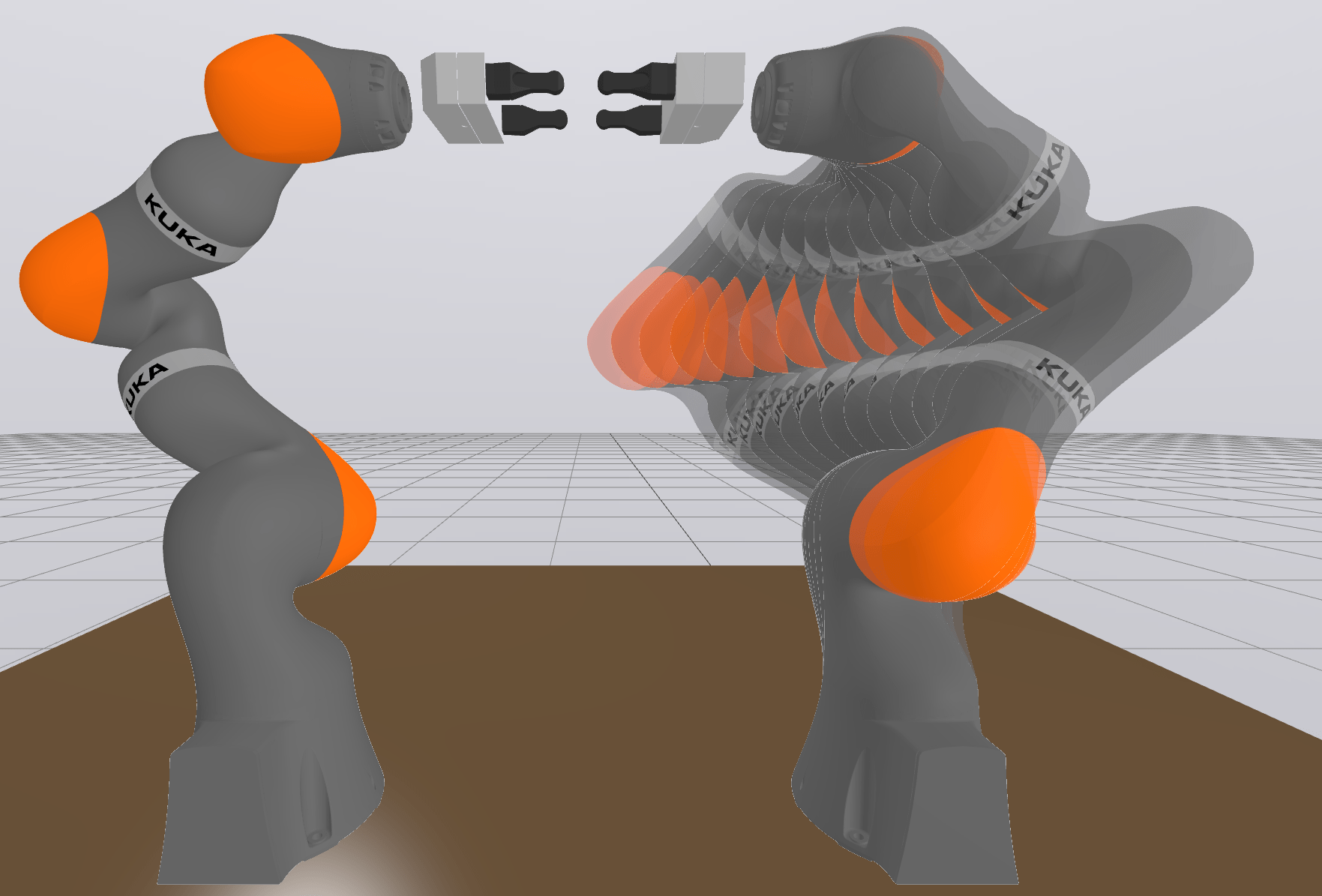
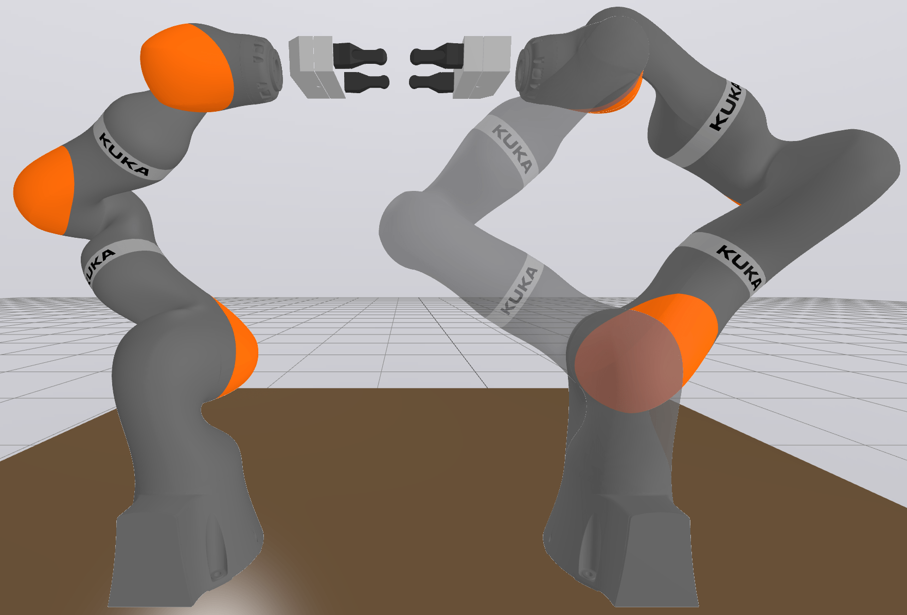
A Worked Example: Bimanual
Motion Planning in Minimal Coordinates for Kinematically-Constrained Systems
Thomas Cohn, Robot Locomotion Group, MIT CSAIL
\(\phi(q_c,\psi_s)=\big(q_c,\ \operatorname{IK}({}^W\!X^{E_s}(q_c),\psi_s)\big)\): 7 controlled joints + 1 self-motion parameter \(\mapsto\) 14 joint angles
Analytic Inverse Kinematics and Self-Motion
Motion Planning in Minimal Coordinates for Kinematically-Constrained Systems
Thomas Cohn, Robot Locomotion Group, MIT CSAIL
Analytic IK can be written as a function
\[\operatorname{IK}:\operatorname{SE}(3)\times\Psi\times\mathscr{K}\to\mathbb{R}^n,\]
where \(\Psi\) are continuous redundancy parameters and \(\mathscr{K}\) are discrete redundancy parameters.
Choosing \(\psi\in\Psi\) and \(\kappa\in\mathscr{K}\) uniquely specifies an IK solution, resolving the "many-to-one" problem.
Reachability Constraints
Motion Planning in Minimal Coordinates for Kinematically-Constrained Systems
Thomas Cohn, Robot Locomotion Group, MIT CSAIL
- For most robots, \(\operatorname{IK}\) is not defined on all of \(\operatorname{SE}(3)\)
- (Obvious example: a robot arm bolted to a table has limited reach)
- Our framework really requires two key ingredients
- A parameterization (i.e. an IK function)
- An optimization-amenable description of its domain
- What does "optimization-amenable" entail?
- Return a value outside the domain
- Gradient signal back towards the domain
A Straightforward Domain Extension
Motion Planning in Minimal Coordinates for Kinematically-Constrained Systems
Thomas Cohn, Robot Locomotion Group, MIT CSAIL
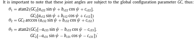
The analytic IK function will have domain limited functions
- \(\arccos(\cdot):[-1,1]\to\mathbb{R}\)
- \(\sqrt{\cdot}:[0,\infty)\to\mathbb{R}\)
Position-based kinematics for 7-DoF serial manipulators with global configuration control, joint limit and singularity avoidance, Faria et al. 2018
Replace with domain-extended versions, e.g.,
\[\arccos(\pi(t))=\left\{\begin{array}{ll}\arccos(-1) & t <=-1\\ \arccos(t) & -1<t<1\\ \arccos(1) & t\ge 1\end{array}\right.\]
\[\sqrt{\pi(t)}=\left\{\begin{array}{ll}\sqrt{0} & t\le 0\\ \sqrt{t} & 0 < t\end{array}\right.\qquad\qquad\]
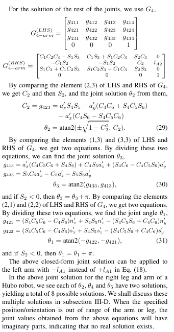
Closed-Form Inverse Kinematic Joint Solution for Humanoid Robots, Ali et al. 2010
"Direct" Reachability Constraint
Motion Planning in Minimal Coordinates for Kinematically-Constrained Systems
Thomas Cohn, Robot Locomotion Group, MIT CSAIL
This extends the domain of \(\operatorname{IK}\) to all of \(\operatorname{SE}(3)\times\Psi\times\mathscr K\), but now it is "incorrect" for nonreachable poses.
Impose the constraint
\[\|\operatorname{FK}(\operatorname{IK}(X,\psi,\kappa))-X\|=0\]
Some properties:
- Positive-measure feasible set
- Always active at a feasible \((X,\psi,\kappa)\) -- even if this isn't on the boundary of the reachable set!
"Probing" Reachability Constraint
Motion Planning in Minimal Coordinates for Kinematically-Constrained Systems
Thomas Cohn, Robot Locomotion Group, MIT CSAIL
Position-based kinematics for 7-DoF serial manipulators with global configuration control, joint limit and singularity avoidance, Faria et al. 2018
Closed-Form Inverse Kinematic Joint Solution for Humanoid Robots, Ali et al. 2010
The analytic IK function will have domain limited functions
- \(\arccos(\cdot):[-1,1]\to\mathbb{R}\)
- \(\sqrt{\cdot}:[0,\infty)\to\mathbb{R}\)
Define probing functions
\[\mathcal{D}_k:\operatorname{SE}(3)\times\Psi\times\mathscr K\to\mathbb R\]
such that
\[\mathcal{D}_k\ge 0,\forall k\Leftrightarrow \textrm{reachable}\]
Constraint only active on boundary: much better for optimization!
Does the Reachability Constraint Matter?
Motion Planning in Minimal Coordinates for Kinematically-Constrained Systems
Thomas Cohn, Robot Locomotion Group, MIT CSAIL
Same chart, same autodiff gradients, same solver (SNOPT)
| Reachability constraint | IrisNp2 (s) | Trajopt (s) |
|---|---|---|
| Direct \(\|\operatorname{FK}(\operatorname{IK}(X,\psi))-X\|=0\) | 1.14 | 1.54 |
| Probing \(\mathcal D_k\ge0\) | 1.03 | 0.98 |
| Boundary (coming up) | 1.08 | 1.24 |
Active everywhere ⇒ 10% slower regions, 50% slower trajopt
Planning with Graphs of Convex Sets
Motion Planning in Minimal Coordinates for Kinematically-Constrained Systems
Thomas Cohn, Robot Locomotion Group, MIT CSAIL
Convex Regions along the Manifold (IRIS-NP2)
Motion Planning in Minimal Coordinates for Kinematically-Constrained Systems
Thomas Cohn, Robot Locomotion Group, MIT CSAIL
The Catch: You Need a Bespoke IK Function
Motion Planning in Minimal Coordinates for Kinematically-Constrained Systems
Thomas Cohn, Robot Locomotion Group, MIT CSAIL
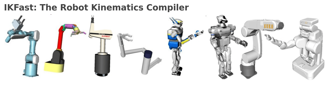
- We want to use our method with all the robots
- We want to allow people to use any IK function they have
- Main target: codegen tools like IKFast
- What do we lose?
- Autodiff support
- Reachability probing functions
The Inverse Function Theorem
Motion Planning in Minimal Coordinates for Kinematically-Constrained Systems
Thomas Cohn, Robot Locomotion Group, MIT CSAIL
Intuition: to differentiate through inverse kinematics, we just need to differentiate through forward kinematics!
(Spivak 1965) Suppose that \(f:\mathbb{R}^n\to\mathbb{R}^n\) is continuously differentiable in an open set containing \(a\), and \(\det f'(a)\ne 0\). Then there is an open set \(V\) containing \(a\) and an open set \(W\) containing \(f(a)\) such that \(f:V\to W\) has a continuous inverse \(f^{-1}:W\to V\) which is differentiable and for all \(y\in W\) satisfies \((f^{-1})'(y)=[f'(f^{-1}(y))]^{-1}\).
Gradients from the IFT
Motion Planning in Minimal Coordinates for Kinematically-Constrained Systems
Thomas Cohn, Robot Locomotion Group, MIT CSAIL
Rough procedure:
- Compute value \(q=\operatorname{IK}({}^W\!X^G,\psi)\)
- Compute augmented Jacobian \(J_A=D\operatorname{FK}_A(q)\)
- Solve \(J_A\,\frac{\partial q}{\partial y}=\big(\frac{\partial X}{\partial y},\frac{\partial\psi}{\partial y}\big)^T\)
Augmented FK \(\operatorname{FK}_A:q\mapsto({}^W\!X^G,\psi)\) is invertible, and
\[D\operatorname{FK}_A=\begin{bmatrix}D\operatorname{FK}\\ D\operatorname{FK}_\psi\end{bmatrix},\qquad D\operatorname{FK}_\psi=[\ldots,0,1,0,\ldots]\ \text{if}\ \psi\ \text{is a joint angle}\]
Direct Numerical Comparison
Motion Planning in Minimal Coordinates for Kinematically-Constrained Systems
Thomas Cohn, Robot Locomotion Group, MIT CSAIL
Procedure:
- Sample reachable configurations
- Sample random partial derivative vectors
- Compute derivatives via autodiff and IFT, compare


Domain Extensions (More Rigorously)
Motion Planning in Minimal Coordinates for Kinematically-Constrained Systems
Thomas Cohn, Robot Locomotion Group, MIT CSAIL
Suppose we write
\[\widehat{\operatorname{IK}}({}^W\!X^G,\psi)=\arg\min_{q}\ \big\|\operatorname{FK}_A(q) - ({}^W\!X^G,\psi)\big\|^2\]
Note: this is not actually what our extensions are doing.
- Our clipping is a greedy projection in some space
- IK-Geo does an iterative least squares projection
- Worst-case naive strategy: bisection to a canonical reachable configuration
We only need a vaguely reasonable answer.
Derivative via Sensitivity Analysis
Motion Planning in Minimal Coordinates for Kinematically-Constrained Systems
Thomas Cohn, Robot Locomotion Group, MIT CSAIL
Suppose we write
\[\widehat{\operatorname{IK}}({}^W\!X^G,\psi)=\arg\min_{q}\ \big\|\operatorname{FK}_A(q) - ({}^W\!X^G,\psi)\big\|^2\]
- Obtain gradient \[D\widehat{\operatorname{IK}}({}^W\!X^G,\psi)=\left(J_A^TJ_A+\sum_{i=1}^nr_iH_i\right)^{-1}J_A^T,\] \(J_A=D\operatorname{FK}_A(q)\), \(H_i=D_q[J_A]_i\), \(r_i\) is the \(i\)th component of the residual \(r=\operatorname{FK}_A(q)-({}^W\!X^G,\psi)\)
- If reachable, \(r_i=0\), so we recover the inverse function theorem when \(J_A\) is nonsingular \[D\widehat{\operatorname{IK}}({}^W\!X^G,\psi)=\left(J_A^TJ_A\right)^{-1}J_A^T=J_A^\dagger=J_A^{-1}\]
Amenable to approximation (Levenberg-Marquardt, residual damping, etc.)
Boundary Reachability
Motion Planning in Minimal Coordinates for Kinematically-Constrained Systems
Thomas Cohn, Robot Locomotion Group, MIT CSAIL
Recall:
- Direct reachability is always active
⮑ Difficult for optimizers to use! - Probing reachability requires privileged information
⮑ Incompatible with black-box IFT treatment
Fun fact:
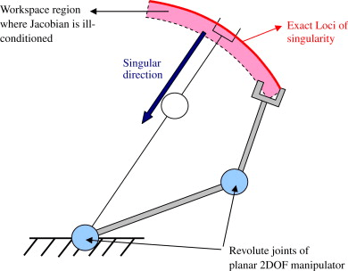
Configurations in the preimage of the workspace boundary have a singular Jacobian!
(Result follows by the open mapping corollary of the IFT.)
Singularity robust algorithm in serial manipulators, Oetomo and Ang 2009
Boundary Reachability
Motion Planning in Minimal Coordinates for Kinematically-Constrained Systems
Thomas Cohn, Robot Locomotion Group, MIT CSAIL
Fun fact:
Configurations in the preimage of the workspace boundary have a singular Jacobian!
(Result follows by the open mapping corollary of the IFT.)
Singularity robust algorithm in serial manipulators, Oetomo and Ang 2009
- Enforce \(-\log\det(J(q)J(q)^T+\epsilon I)\le\tau\) for problem-dependent constants \(\epsilon,\tau\).
- Only active on the boundary (like probing reachability), no IK internals needed
Boundary Reachability in Action
Motion Planning in Minimal Coordinates for Kinematically-Constrained Systems
Thomas Cohn, Robot Locomotion Group, MIT CSAIL
Boundary Reachability Results
Motion Planning in Minimal Coordinates for Kinematically-Constrained Systems
Thomas Cohn, Robot Locomotion Group, MIT CSAIL
| Gradient method (bimanual iiwa) | IrisNp2 (s) | Trajopt (s) |
|---|---|---|
| Autodiff baselines (bespoke IK) | ||
| Autodiff, direct reachability | 1.14 | 1.54 |
| Autodiff, probing reachability | 1.03 | 0.98 |
| Autodiff, boundary reachability | 1.08 | 1.24 |
| IFT, direct reachability | ||
| Zero gradients | 4.11 | 1.35 |
| Pseudoinverse | 4.12 | 1.31 |
| LM constant | 3.12 | 1.42 |
| LM SVT | 2.22 | 1.49 |
| Residual damping | 1.58 | 1.76 |
| Anisotropic damping | 1.72 | 2.52 |
| Full Newton | 1.71 | 1.43 |
| IFT, boundary reachability | ||
| Zero gradients | 1.64 | 1.20 |
| Pseudoinverse | 1.75 | 1.23 |
| LM constant | 2.51 | 1.31 |
| LM SVT | 1.29 | 1.21 |
| Residual damping | 1.15 | 1.24 |
| Anisotropic damping | 1.15 | 1.23 |
| Full Newton | 1.17 | 1.20 |
- IrisNp2 is a reachability optimization "challenge" problem
- Can match autodiff performance, with
- IFT gradients
- Boundary reachability
- Gradient regularization
Box Pickup with Stability Constraints
Motion Planning in Minimal Coordinates for Kinematically-Constrained Systems
Thomas Cohn, Robot Locomotion Group, MIT CSAIL
The Benchmark Suite
Motion Planning in Minimal Coordinates for Kinematically-Constrained Systems
Thomas Cohn, Robot Locomotion Group, MIT CSAIL
Optimization IK
- Framework suite: 5 robots × 3 solvers
- UR5e grasp selection (EAIK)
Planning
- IRIS-NP2 counterexample search
- iiwa bimanual trajopt (autodiff / IFT)
- RB-Y1 constrained trajopt (IKFast)
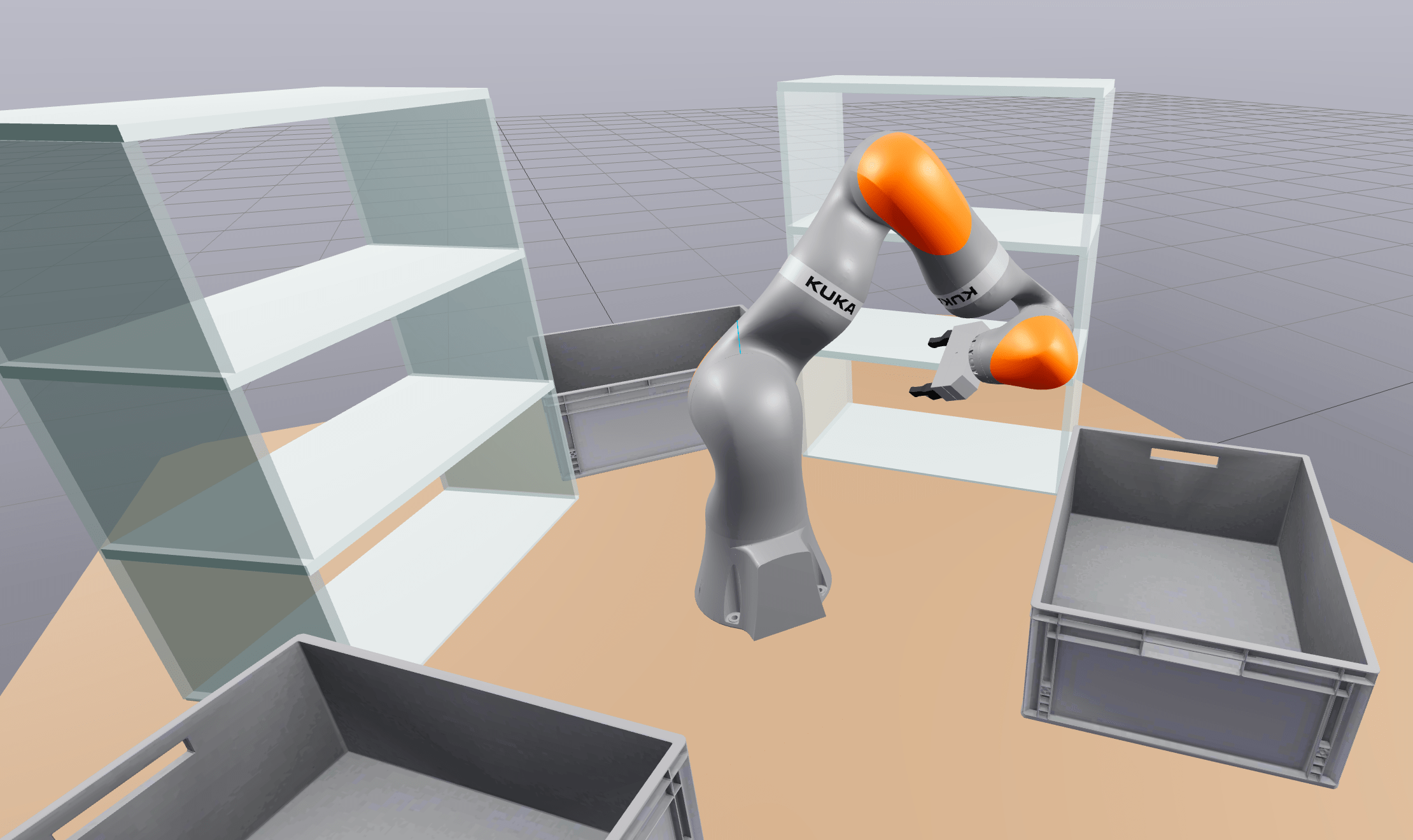
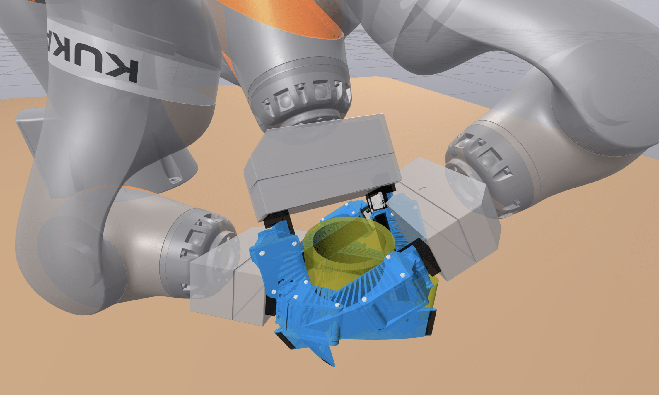
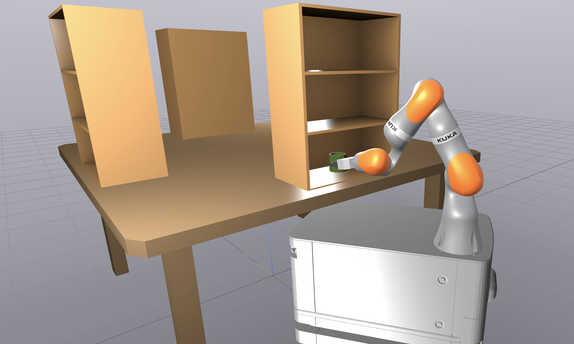
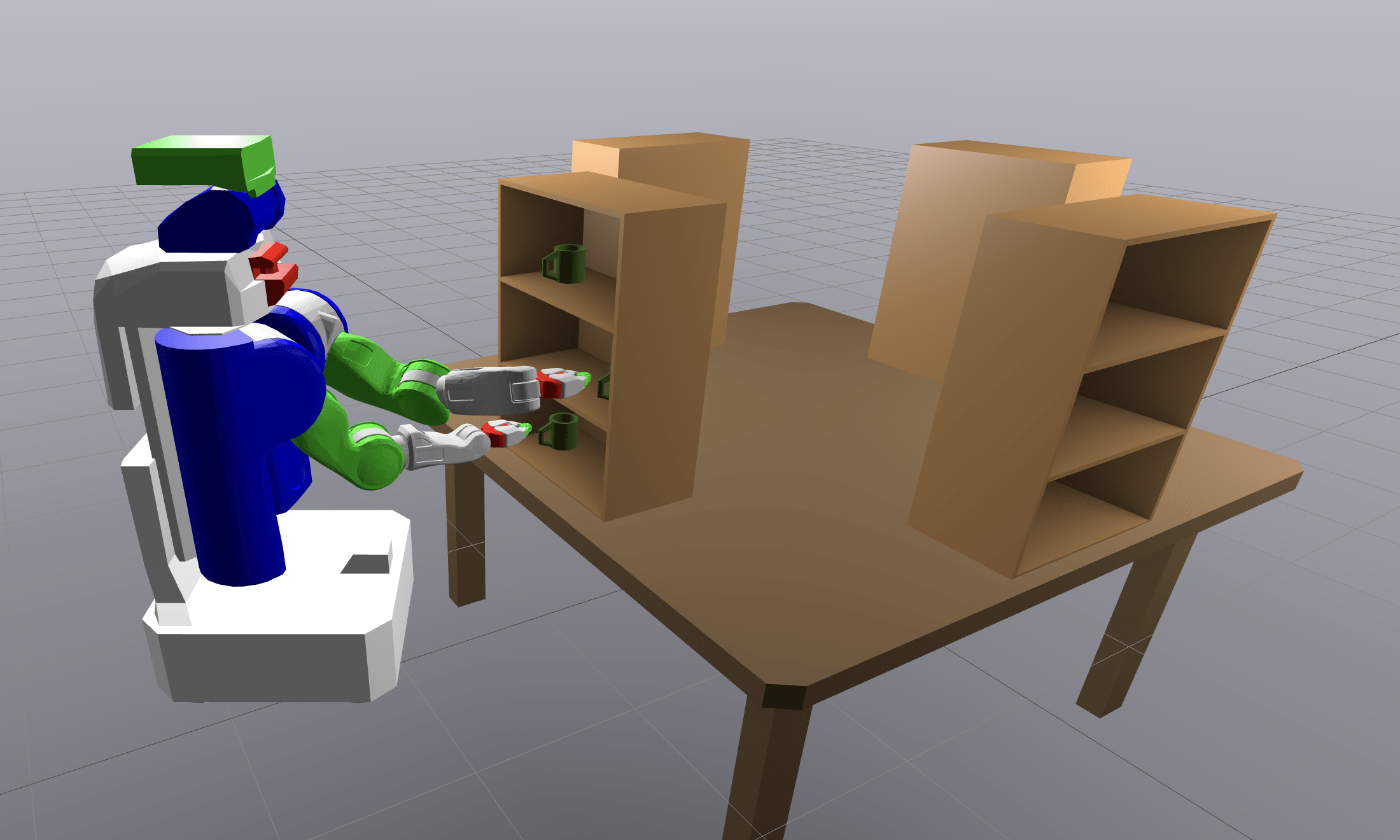
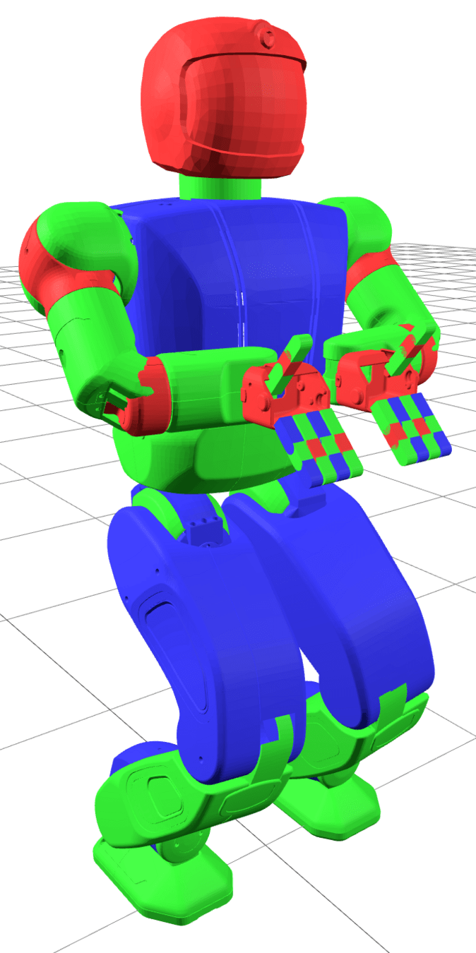

Arm on a table · grasp selection · mobile manipulator · bimanual mobile manipulator · humanoid stability · UR5e grasp selection (EAIK)
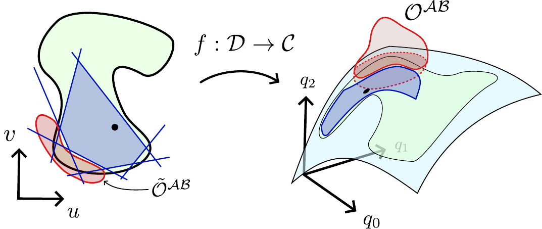


IRIS-NP2 regions · iiwa bimanual · RB-Y1 box pickup
Highlight 1: IRIS-NP2 Counterexample Search
Motion Planning in Minimal Coordinates for Kinematically-Constrained Systems
Thomas Cohn, Robot Locomotion Group, MIT CSAIL
- Finding nearby constraint violations and wall them off with a hyperplane
- Must work outside the reachable set
| Gradient outside the reachable set | IrisNp2 (s) |
|---|---|
| Bespoke autodiff, probing reach | 1.03 |
| IFT, zero gradient, direct reach | 4.11 |
| IFT, pseudoinverse, direct reach | 4.12 |
| IFT, residual damping, direct reach | 1.58 |
| IFT, residual damping, boundary reach | 1.15 |
4× from the gradient choice alone
Highlight 2: UR5e Grasp IK (EAIK)
Motion Planning in Minimal Coordinates for Kinematically-Constrained Systems
Thomas Cohn, Robot Locomotion Group, MIT CSAIL

- Collision-free grasp on a mug
- Black-box IK (EAIK), 6 variables
- 100 targets × 10 guesses, SNOPT
| Formulation | Success (1 init) | Success (3 init) | Mean cost | Mean t (s) | Median t (s) |
|---|---|---|---|---|---|
| C-space baseline | 46.5% | 86% | 12.68 | 0.357 | 0.105 |
| IFT, direct reach. | 61.4% | 93% | 13.30 | 0.719 | 0.100 |
| IFT, boundary reach. | 63.2% | 90% | 13.53 | 0.776 | 0.110 |
- +15 pp success, same median time, 2× mean time
- Failures hit the iteration limit, not the clock
Also: other IK setups (arm on a table, mobile manipulator, bimanual mobile manipulator, humanoid stability)
Highlight 3: Bimanual Trajopt vs. Tolerances
Motion Planning in Minimal Coordinates for Kinematically-Constrained Systems
Thomas Cohn, Robot Locomotion Group, MIT CSAIL
- Bimanual iiwa, autodiff gradients (best case)
- 137 variables, 1,217 constraint rows
| Solver / setting | Converged | Feasible | Time (s) | Cost |
|---|---|---|---|---|
| SNOPT, optimality tol 1e-1 … 1e-3 | yes | yes | 2.0 | 1.59 |
| SNOPT, optimality tol 1e-6 (default) | no | yes | 19.4 | 1.36 |
| IPOPT, penalty line search | yes | yes | 40.9 | 1.36 |
| IPOPT, default (filter line search) | no | yes | 60.1 | 1.38 |
- Feasible throughout; optimality is what can't be certified
- Hacky SNOPT-in-a-box probe: ~1.2 s at any tolerance. Suggestive, not trusted.
Why Trust Regions?
Motion Planning in Minimal Coordinates for Kinematically-Constrained Systems
Thomas Cohn, Robot Locomotion Group, MIT CSAIL
- Outside the reachable set:
value from a cheap projection, gradient from the idealized \(\widehat{\operatorname{IK}}\) - Inexact gradients by construction
- Line searches stall
| Instance | Symptom |
|---|---|
| iiwa trajopt (SNOPT) | tol 1e-3: 2 s → tol 1e-6: 19 s, not converged |
| RB-Y1 trajopt (SNOPT) | 52 failures: 42 time limit, 8 iteration limit, 0 infeasible |
| UR5e IK (SNOPT) | iteration-limit exits 177 / 137 / 114 per 1,000; clock: 1 |
| IRIS-NP2 (SNOPT) | 4.11 s vs 1.15 s from the gradient choice alone |
Thanks to My Collaborators on this Project
Motion Planning in Minimal Coordinates for Kinematically-Constrained Systems
Thomas Cohn, Robot Locomotion Group, MIT CSAIL











Motion Planning in Minimal Coordinates for Kinematically-Constrained Systems
Thomas Cohn
September 23, 2026
Presentation for the MIT REx Lab group meeting
Robot Locomotion Group