Parameterizing Constraint Manifolds with the Inverse Function Theorem

Thomas Cohn

May 1, 2026
Task-Space Constraints
Learning the Metric of Task Constraint Manifolds for Constrained Motion Planning, Zha et. al.
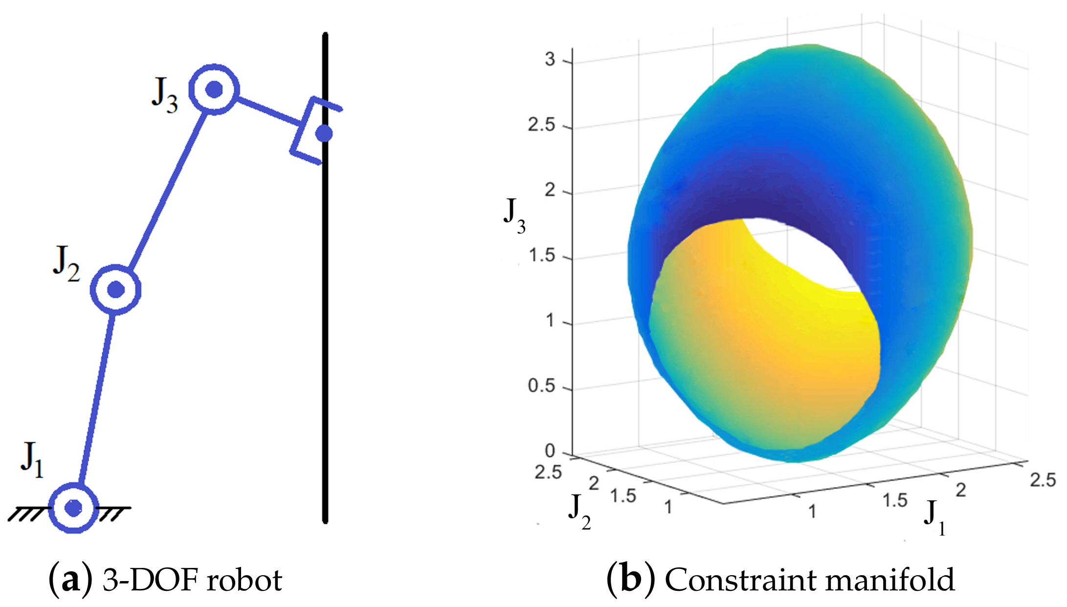
Planning with Kinematic Constraints
Collision-Free Motion Planning Problem:
\[\begin{array}{rl}\min_\gamma & L(\gamma)\\ \operatorname{s.t.} & \gamma:[0,1]\to\mathbb R^n\\ & \gamma(0)=q_0,\gamma(1)=q_1\\ & g(\gamma(t))\le 0,\forall t\in[0,1]\end{array}\]
Constrained Collision-Free Motion Planning Problem:
\[\begin{array}{rl}\min_\gamma & L(\gamma)\\ \operatorname{s.t.} & \gamma:[0,1]\to\mathbb R^n\\ & \gamma(0)=q_0,\gamma(1)=q_1\\ & g(\gamma(t))\le 0,\forall t\in[0,1]\\ & h(\gamma(t))=0,\forall t\in[0,1]\end{array}\]
Some Additional Structure
Constrained Collision-Free Motion Planning Problem:
\[\begin{array}{rl}\min_\gamma & L(\gamma)\\ \operatorname{s.t.} & \gamma:[0,1]\to\mathbb R^n\\ & \gamma(0)=q_0,\gamma(1)=q_1\\ & g(\gamma(t))\le 0,\forall t\in[0,1]\\ & h(\gamma(t))=0,\forall t\in[0,1]\end{array}\]
- Constraint manifold \(\mathcal M=\{q\in\mathbb R^n:h(q)=0\}\)
- Parametrization \(\xi:\mathbb R^m\to\mathbb R^n\), reachable domain \(\mathcal U\subseteq\mathbb R^m\)
- Require:
- \(\xi\) is differentiable almost everywhere
- \(\xi(\mathcal U)\subseteq\mathcal M\)
Parameterized Planning Problem
\[\begin{array}{rl}\min_\gamma & L(\gamma)\\ \operatorname{s.t.} & \gamma:[0,1]\to\mathbb R^n\\ & \gamma(0)=q_0,\gamma(1)=q_1\\ & g(\gamma(t))\le 0,\forall t\in[0,1]\\ & h(\gamma(t))=0,\forall t\in[0,1]\end{array}\]
- Constraint manifold \(\mathcal M=\{q\in\mathbb R^n:h(q)=0\}\)
- Parametrization \(\xi:\mathbb R^m\to\mathbb R^n\), reachable domain \(\mathcal U\subseteq\mathbb R^m\)
- Require:
- \(\xi\) is differentiable almost everywhere
- \(\xi(\mathcal U)\subseteq\mathcal M\)
\[\begin{array}{rl}\min_{\tilde\gamma}& L(\xi\circ\tilde\gamma)\\ \operatorname{s.t.} & \tilde\gamma:[0,1]\to\mathcal U\\ & \tilde\gamma(0)=\tilde q_0,\tilde\gamma(1)=\tilde q_1\\ & g((\xi\circ\tilde\gamma)(t))\le 0,\forall t\in[0,1]\\ & h((\xi\circ\tilde\gamma)(t))=0,\forall t\in[0,1]\end{array}\]
Parameterized Planning Problem
\[\begin{array}{rl}\min_{\tilde\gamma}& L(\xi\circ\tilde\gamma)\\ \operatorname{s.t.} & \tilde\gamma:[0,1]\to\mathcal U\\ & \tilde\gamma(0)=\tilde q_0,\tilde\gamma(1)=\tilde q_1\\ & g((\xi\circ\tilde\gamma)(t))\le 0,\forall t\in[0,1]\\ & h((\xi\circ\tilde\gamma)(t))=0,\forall t\in[0,1]\end{array}\]
"Reachability Constraint"
Assume we can construct \(\tilde q_i\) such that \(\xi(\tilde q_i)=q_i\), \(i\in\{0,1\}\).
Becomes more Complicated
Eliminated by Construction: \(\tilde\gamma(t)\in\mathcal U\Rightarrow h((\xi\circ\tilde\gamma)(t))=0\)
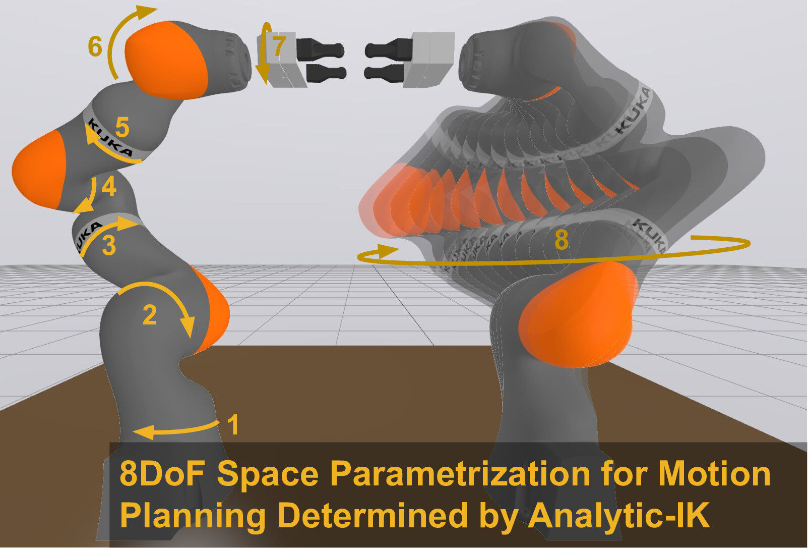
Building Parametrizations with Analytic IK
Analytic IK can be written as a function
\[\operatorname{IK}:\operatorname{SE}(3)\times\mathcal{C}\times\mathcal{D}\to\mathbb{R}^n,\]
where \(\mathcal{C}\) are continuous redundancy parameters and \(\mathcal{D}\) are discrete redundancy parameters.
Forward kinematics can be written as a function
\[\operatorname{FK}:\mathbb{R}^n\to\operatorname{SE}(3)\]
Note: we often have \(n>6\), so \(\operatorname{FK}\) is not locally invertible.
Redundancy Parameterization
Analytic IK can be written as a function
\[\operatorname{IK}:\operatorname{SE}(3)\times\mathcal{C}\times\mathcal{D}\to\mathbb{R}^n,\]
where \(\mathcal{C}\) are continuous redundancy parameters and \(\mathcal{D}\) are discrete redundancy parameters.
\(\mathcal{C}\) and \(\mathcal{D}\) parameterize the self-motion of a robot arm:
Specialized Redundancy Parameterizations
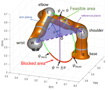
Safety-Enhanced Human-Robot Interaction Control of Redundant Robot for Teleoperated Minimally Invasive Surgery, Su et al.
Redundancy parameterization and inverse kinematics of 7-DOF revolute manipulators, Elias and Wen.
General Redundancy Parameterizations
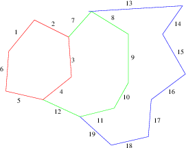
Key idea:
- Solve some (length-6) chains with IK
- All remaining joint angles are self-motion parameters
A kinematics-based probabilistic roadmap method for high DOF closed chain systems, Xie and Amato.
Differentiating through IK
Reminder: we want to solve
\[\begin{array}{rl}\min_{\tilde\gamma}& L(\xi\circ\tilde\gamma)\\ \operatorname{s.t.} & \tilde\gamma:[0,1]\to\mathcal U\\ & \tilde\gamma(0)=\tilde q_0,\tilde\gamma(1)=\tilde q_1\\ & g((\xi\circ\tilde\gamma)(t))\le 0,\forall t\in[0,1]\end{array}\]
To use gradient-based optimization, need to compute \(D\xi\)
If you implement analytic IK by hand, easy to make it compatible with an autodiff framework
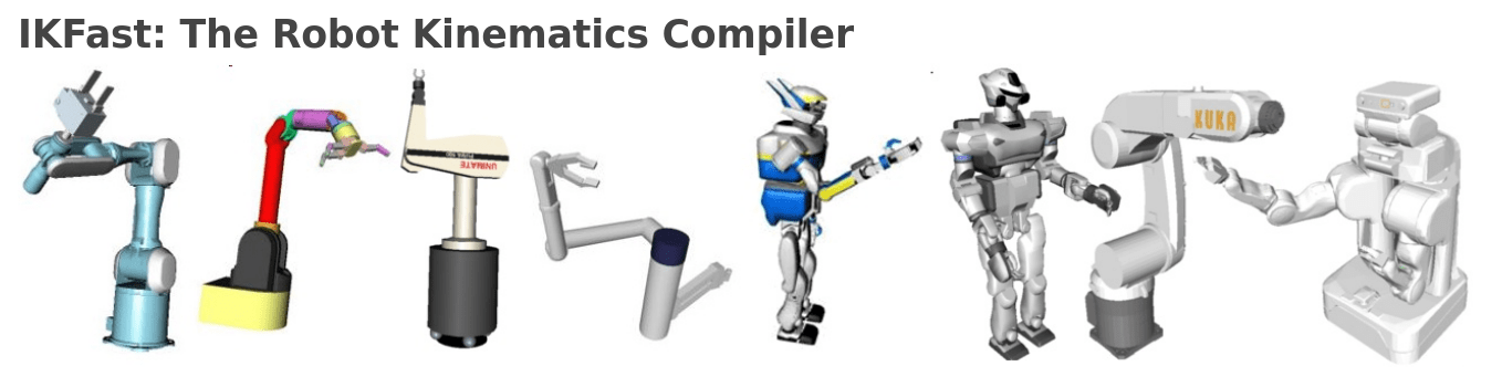
Black-Box IK Functions
- We want to use our method with all the robots
- We want to allow people to use any IK function they have
- Main target: codegen tools like IKFast
- Modifying to support autodiff is a major task!
The Inverse Function Theorem
Intuition: to differentiate through inverse kinematics, we just need to differentiate through forward kinematics!
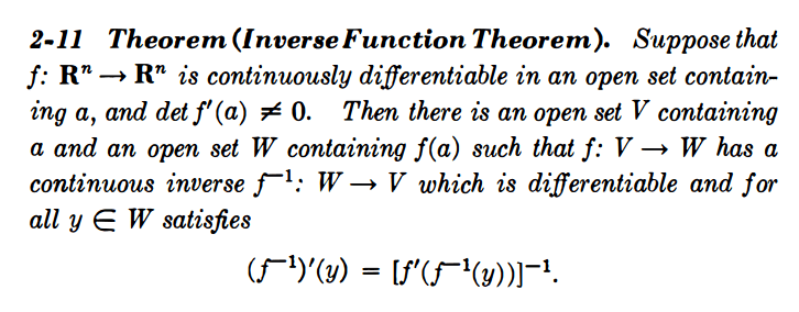
Calculus on Manifolds, Michael Spivak
Rough procedure:
- Compute value \(q=\operatorname{IK}({}^W\!X^G)\)
- Compute Jacobian \(J=D\operatorname{FK}(q)\)
- Invert: \(D\operatorname{IK}({}^W\!X^G)=J^{-1}\)
Augmented Forward Kinematics
For invertibility, need the augmented forward kinematics
\[\operatorname{FK}_A:q\mapsto({}^W\!X^G,\psi),\]
which returns the end-effector pose and the self-motion parameters.
Augmented Forward Kinematics
We want the output partials
\[\frac{\partial q}{\partial y}=D\operatorname{IK}({}^W\!X^G,\psi)\frac{\partial ({}^W\!X^G,\psi)}{\partial y}=(D\operatorname{FK}_A(q))^{-1}\frac{\partial ({}^W\!X^G,\psi)}{\partial y}\]
Suppose \(q=\operatorname{IK}({}^W\!X^G,\psi)\), and we're given partials \(\frac{\partial ({}^W\!X^G,\psi)}{\partial y}\).
To avoid the matrix inversion, we solve the linear system
\[D\operatorname{FK}_A(q)\frac{\partial q}{\partial y}=\frac{\partial ({}^W\!X^G,\psi)}{\partial y}\]
Augmented Forward Kinematics
Remember, we're using the augmented forward kinematics
\[\operatorname{FK}_A:q\mapsto({}^W\!X^G,\psi),\]
which returns the end-effector pose and the self-motion parameters.
\(D\operatorname{FK}_A\) is well structured:
\[D\operatorname{FK}_A=\begin{bmatrix}D\operatorname{FK}\\ D\psi\end{bmatrix}\]
If we use the \(n\)th joint as the self motion parameter, then
\[D\psi=[\ldots,0,1,0,\ldots]\]
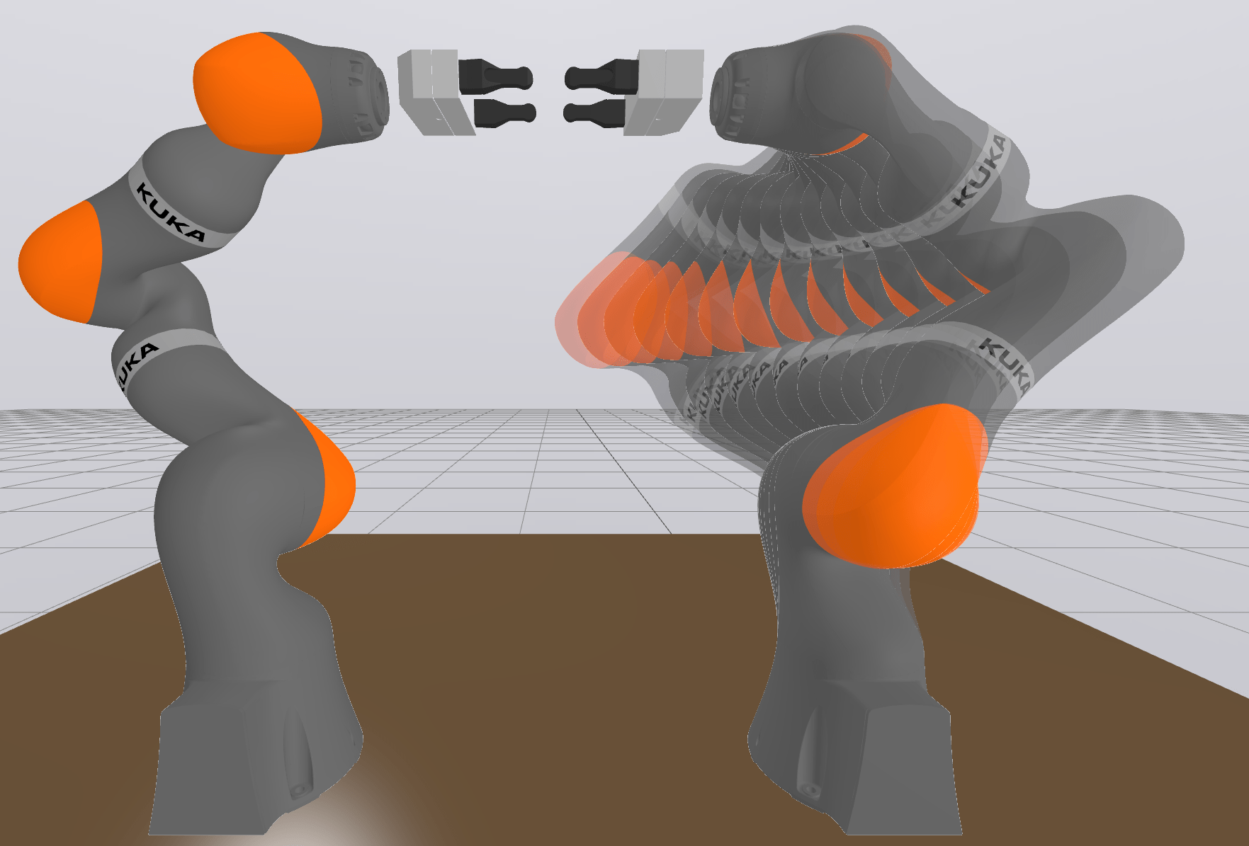
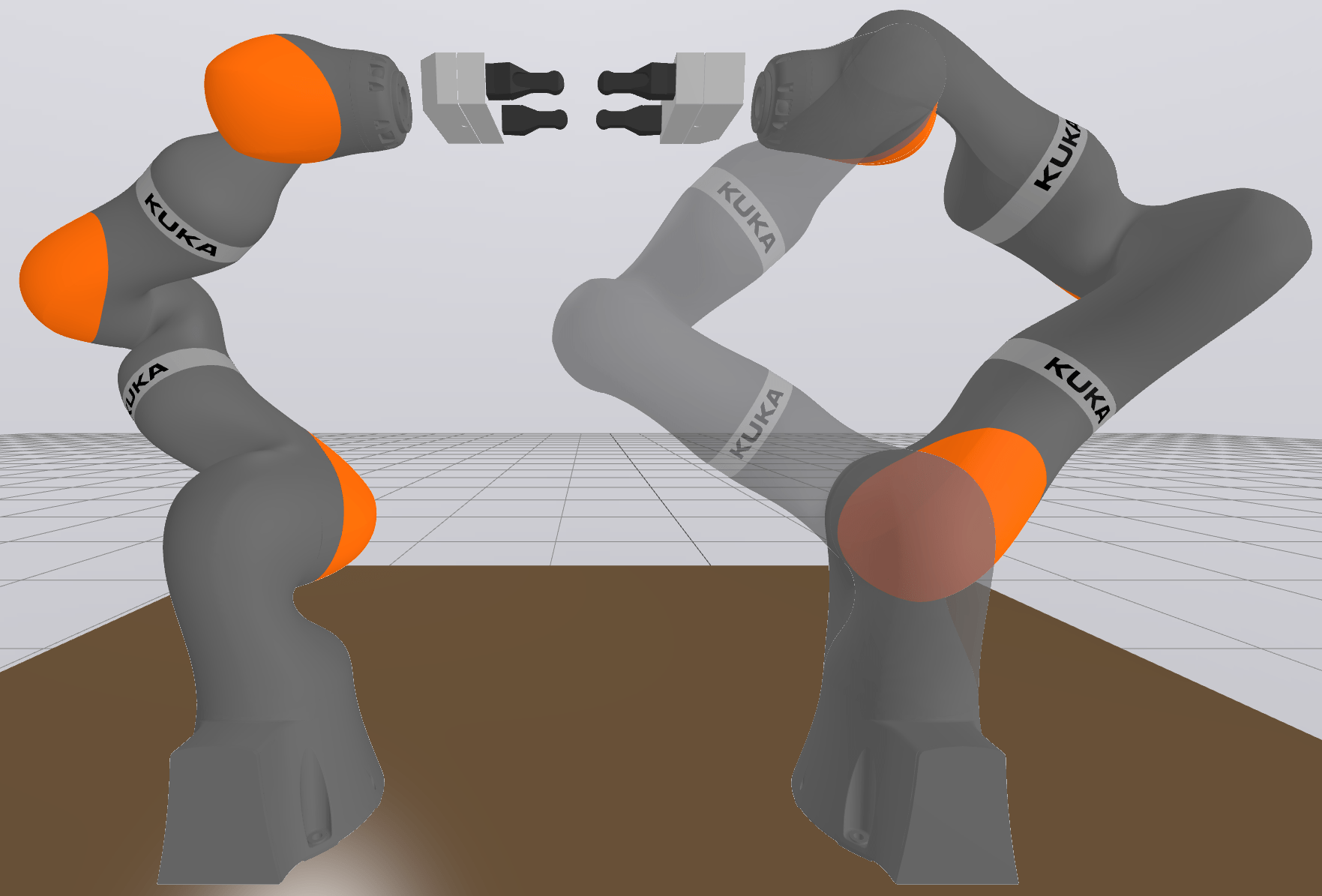
A Worked Example: Bimanual
Consider the leader-follower bimanual iiwa setup:
Notation
- \(q_c,q_s\in\mathbb R^7\) controlled, subordinate joint angles
- \(E_c,E_s\) end-effector frames
- \(\psi_s\) subordinate arm self-motion
- \({}^{E_c}\!X^{E_s}\) fixed relative end-effector transform
A Worked Example: Bimanual
- \(q_c,q_s\in\mathbb R^7\) controlled, subordinate joint angles
- \(E_c,E_s\) end-effector frames
- \(\psi_s\) subordinate arm self-motion
- \({}^{E_c}\!X^{E_s}\) fixed relative end-effector transform
- \(\operatorname{FK}_c\) is the ordinary FK for the controlled arm
- \(\operatorname{FK}_A\) is the augmented FK for the subordinate arm
- \(\operatorname{IK}\) is the analytic IK for the subordinate arm
The full parameterization can be written as \((q_c,q_s)=\xi(q_c,\psi_s)\),
\[\xi(q_c,\psi_s)=(q_c,\operatorname{IK}({}^W\!X^{E_s}(q_c),\psi_s))=(q_c,\operatorname{IK}(\operatorname{FK}_c(q_c){}^{E_c}\!X^{E_s},\psi_s))\]
A Worked Example: Bimanual
The full parameterization can be written as \((q_c,q_s)=\xi(q_c,\psi_s)\),
\[\xi(q_c,\psi_s)=(q_c,\operatorname{IK}({}^W\!X^{E_s}(q_c),\psi_s))=(q_c,\operatorname{IK}(\operatorname{FK}_c(q_c){}^{E_c}\!X^{E_s},\psi_s))\]
Derivative block structure:
\[D\xi=\frac{\partial(q_c,q_s)}{\partial(q_c,\psi_s)}=\begin{bmatrix}I\quad 0\\ \frac{\partial q_s}{\partial(q_c,\psi_s)}\end{bmatrix}\]
Apply the chain rule:
\[\frac{\partial q_s}{\partial (q_c,\psi_s)}=\frac{\partial q_s}{\partial({}^W\!X^{E_s},\psi_s)}\frac{\partial({}^W\!X^{E_s},\psi_s)}{\partial (q_c,\psi_s)}\]
A Worked Example: Bimanual
Apply the chain rule:
\[\frac{\partial q_s}{\partial (q_c,\psi_s)}=\frac{\partial q_s}{\partial({}^W\!X^{E_s},\psi_s)}\frac{\partial({}^W\!X^{E_s},\psi_s)}{\partial (q_c,\psi_s)}\]
Second term:
\[\frac{\partial({}^W\!X^{E_s},\psi_s)}{\partial (q_c,\psi_s)}=\begin{bmatrix}D\operatorname{FK}_c(q_c){}^{E_s}\!X^{E_c} & 0\\ 0 & 1\end{bmatrix}\]
First term:
\[\frac{\partial q_s}{\partial({}^W\!X^{E_s},\psi_s)}=\left(\frac{\partial({}^W\!X^{E_s},\psi_s)}{\partial q_s}\right)^{-1}=\left(D\operatorname{FK}_A(q_s)\right)^{-1}\]
A Worked Example: Bimanual
Putting it all together
\[D\xi=\begin{bmatrix}I\qquad\qquad\qquad 0\\ \\ \left(D\operatorname{FK}_A(q_s)\right)^{-1}\begin{bmatrix}D\operatorname{FK}_c(q_c){}^{E_s}\!X^{E_c} & 0\\ 0 & 1\end{bmatrix}\end{bmatrix}\]
We can avoid the matrix inversion.
Given incoming partials \((\frac{\partial q_c}{\partial y},\frac{\partial \psi_s}{\partial y})\), obtain \(\frac{\partial q_s}{\partial y}\) by solving the linear system
\[D\operatorname{FK}_A(q_s)\frac{\partial q_s}{\partial y}=\begin{bmatrix}D\operatorname{FK}_c(q_c){}^{E_s}\!X^{E_c} & 0\\ 0 & 1\end{bmatrix}\begin{bmatrix}\frac{\partial q_c}{\partial y}\\ \frac{\partial \psi_s}{\partial y}\end{bmatrix}\]
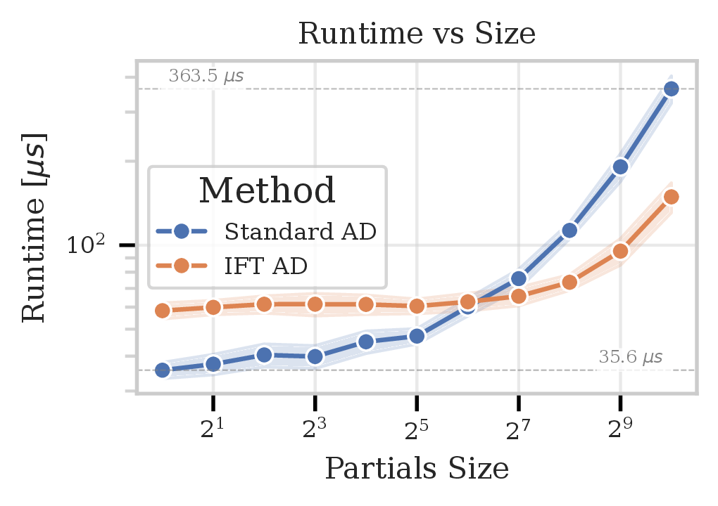
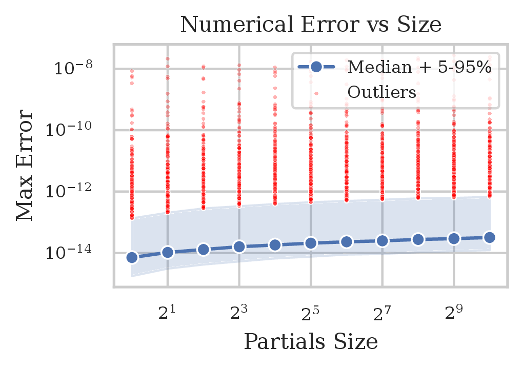
Direct Numerical Comparison
Procedure (for \(\xi:\tilde q\mapsto q\)):
- Sample reachable configurations \(\left\{\tilde q_i\right\}_{i=1}^{10\,000}\)
- For each \(i\), sample random partial vectors \(\frac{\partial \tilde q_i}{\partial y_{ij}}\in\mathbb R^{2^j}\)
- Compute \(\frac{\partial q_i}{\partial y_{ij}}\) via autodiff and IFT, compare
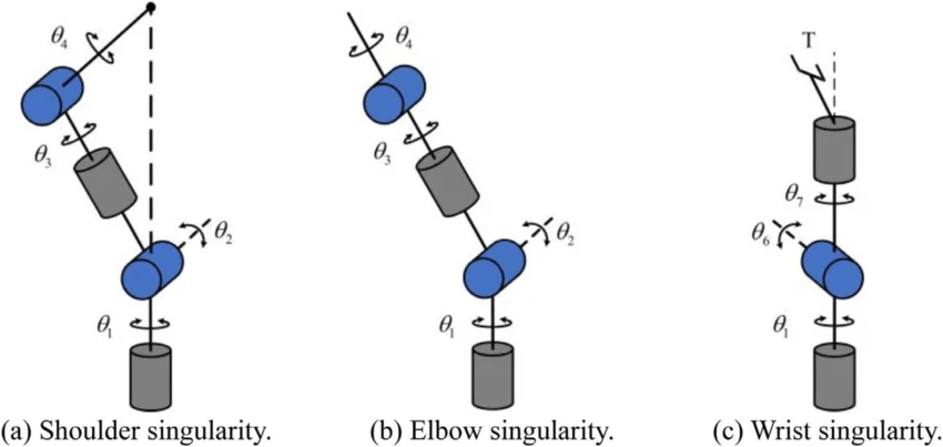
What about Singularities?
\(D\operatorname{FK}\) loses rank
Kinematic singularity: end-effector loses a degree of freedom
Representational singularity: self-motion not represented by redundancy parameter
\(D\operatorname{FK}_A\) loses rank, \(D\operatorname{FK}\) may not
Joints limits and singularity avoidance, Takla and Layous
A "Pseudoinverse" Function Theorem?
A naive idea...
- Can't invert a matrix?
- Take the pseudoinverse instead!
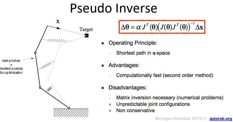
Differences from numerical IK via Jacobian pseudoinverse
- Jacobian not full rank -- we know we're at singularity
- Not modifying joint angles, just pushing through gradients
Intuition: preserve gradient flow along directions we can, truncate directions we cannot
EECS 367 Lecture 12, Jenkins
Our prior work:
- Extend IK domain via greedy projection
- Gradients truncated by this step, rely on other gradient signal
- E.g. \(D||\operatorname{FK}(\operatorname{IK}({}^W\!X^G,\psi))-{}^W\!X^G||_F^2\) still gives signal from the latter term.
- Empirically: not good enough with IFT!
- Explicit domain constraints ("probing functions") provide external signal
- Not an option for a generic IK function!
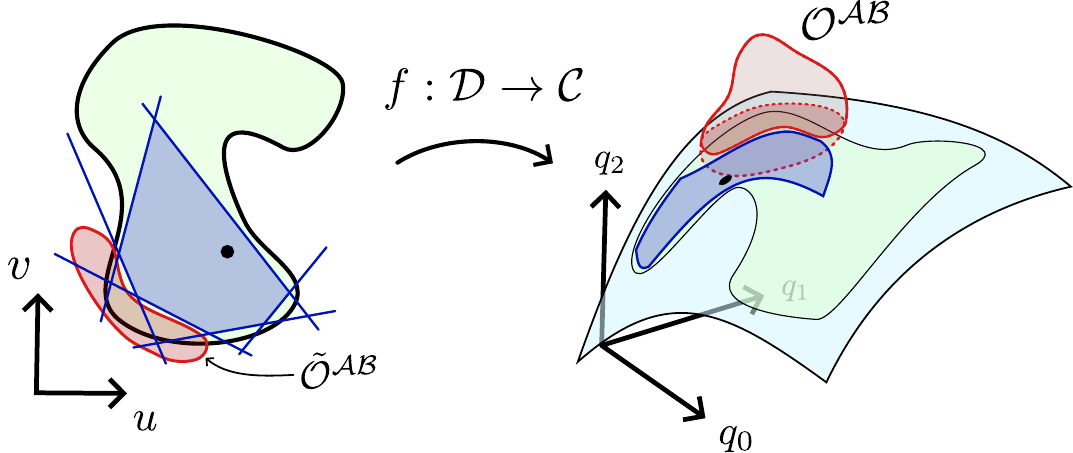
Non-Reachable Configurations?
Idealized Domain Extension
Ignore self-motion parameter for now. Suppose we write
\[\hat{\operatorname{IK}}({}^W\!X^G) = \left\{ \begin{array}{ll} \begin{array}{rl} \displaystyle \arg\min_{q} & \|\operatorname{FK}(q) - {}^W\!X^G\|^2 \\ \text{s.t.} & q \in \mathbb{T}^n \end{array} & {}^W\!X^G\;\text{not reachable} \\ \operatorname{IK}({}^W\!X^G) & {}^W\!X^G\;\text{reachable} \end{array} \right. \]
Note: this is not actually what our extensions are doing.
- Our clipping is a greedy projection in some space
- IK-Geo does an iterative least squares projection
- Taking the real part of complex solutions for polynomial IK is some sort of projection? (More on this in 3-6 months...)
But perhaps it's a reasonable approximation?
\[\begin{array}{rl} \displaystyle \arg\min_{q} & \|\operatorname{FK}(q) - {}^W\!X^G\|^2 \\ \text{s.t.} & q \in \mathbb{T}^n \end{array}\]
Derivative via Sensitivity Analysis
- \(J\) kinematic Jacobian, \(H\) kinematic Hessian
- First order optimality conditions: \[J(q)(\operatorname{FK}(q)-{}^W\!X^G)=0\]
- Apply implicit function theorem, push some symbols...
- Obtain gradient \[D\hat{\operatorname{IK}}({}^W\!X^G)=\left(J(q)^TJ(q)+\sum_{i=1}^nr_iH_i(x)\right)^{-1}J(q),\] \(r_i\) is the \(i\)th component of the residual \(\operatorname{FK}(q)-{}^W\!X^G\)
Derivative via Sensitivity Analysis
- Obtain gradient \[D\hat{\operatorname{IK}}({}^W\!X^G)=\left(J(q)^TJ(q)+\sum_{i=1}^nr_iH_i(x)\right)^{-1}J(q),\] \(r_i\) is the \(i\)th component of the residual \(r=\operatorname{FK}(q)-{}^W\!X^G\)
- If reachable, \(r_i=0\), so \[D\hat{\operatorname{IK}}({}^W\!X^G)=\left(J(q)^TJ(q)\right)^{-1}J(q)=J(q)^\dagger\] So taking the pseudoinverse is doing something reasonable!
- Fancier approximations...
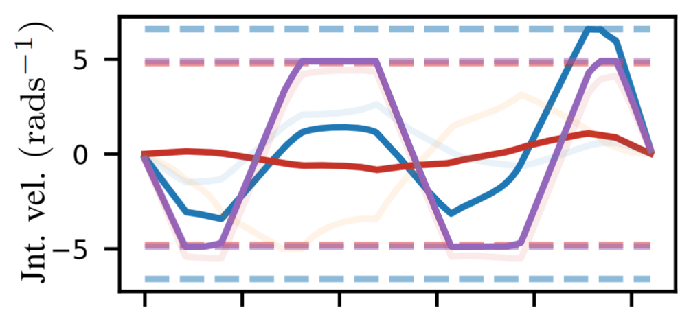
Damping and Residuals
- Obtain gradient \[D\hat{\operatorname{IK}}({}^W\!X^G)=\left(J(q)^TJ(q)+\sum_{i=1}^nr_iH_i(x)\right)^{-1}J(q),\] \(r_i\) is the \(i\)th component of the residual \(r=\operatorname{FK}(q)-{}^W\!X^G\)
- Fancier approximations...
- Damping \[D\hat{\operatorname{IK}}({}^W\!X^G):=(J(q)^TJ(q)+\lambda(q) I)^{-1}J(q)^T\]
- Classic Levenbarg-Marquardt: constant \(\lambda\)
- Singular Value Thresholding: \(\lambda(q)\) grows as \(\sigma_{\min}(J(q))\searrow 0\)
- Residual Damping: \(\lambda(q)\) scaled by \(\|r\|^2\)
- Damping \[D\hat{\operatorname{IK}}({}^W\!X^G):=(J(q)^TJ(q)+\lambda(q) I)^{-1}J(q)^T\]
Damping and Residuals
- Fancier approximations...
- Anistropic Damping \[J=U\Sigma V^T,\quad \Lambda_j=\lambda(\|r\|^2+3(u_j^Tr)^2),\quad \Lambda=\operatorname{diag}(\Lambda_j),\vphantom{\int}\] \[D\hat{\operatorname{IK}}({}^W\!X^G)=(\tilde J^T\tilde J+V\Lambda V^T)^{-1}\tilde J^T\]
- Regularized Full Newton Step: \[D\hat{\operatorname{IK}}({}^W\!X^G)=\left(J(q)^TJ(q)+\sum_{i=1}^nr_iH_i(x)+\lambda I\right)^{-1}J(q),\]
Taking a Step Back
- What exactly did we do here?
- Numerical IK with Jacobian Psuedoinverse
- Use \(J^\dagger\) to modify joint angles
- Pseudoinverse handles redundancy
- Autodiff with Jacobian Pseudoinverse
- Use \(J^\dagger\) to propagate gradients
- Pseudoinverse handles singularities
- More advanced methods also correspond to numerical IK
- A possible intuition/explanation?
- Within reachable set, do analytic IK
- Outside of reachable set, do numerical IK
Downstream Experiments
IRIS-NP2: Generating convex collision-free polytopes in parameterized C-space
Kinematic trajectory optimization
TOPPRA: Retiming trajectories for robot dynamics limits
A New Approach to Time-Optimal Path Parameterization based on Reachability Analysis, Pham and Pham
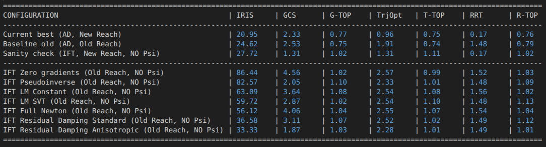
- Residual damping performs best for IRIS-NP2
- Full Newton method less effective
- Maybe because not truly least-squares projection?
- GCS runtime is a rough proxy for region quality
- All methods effective for TrajOpt, TOPP-RA
- Unsurprising due to feasible start
Runtimes: Bimanual iiwa Setup
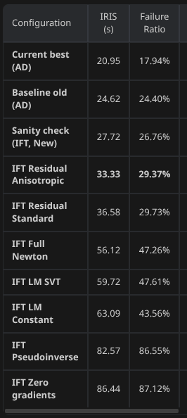
For the IRIS-NP2 Afficionados
- IRIS-NP2 requires solving "counterexample search programs"
- Numerically challenging
- Must work outside of reachable set
- Residual damping still most performant
- Full Newton method not much better than Levenberg-Marquardt
- Pseudoinverse and Zero Gradients reliant on random sampling
RB-Y1
Param: torso + both arms following frame between gripper
Conclusions and What's Next
- The inverse function theorem works
- We can take derivatives this way
- Can handle numerical issues at critical points
- Let's do it with robots on hardware
- Hope to have some cool videos with Ruby
- Candidates for a single, general solution to IK
- IK-Geo
- Polynomial IK
Parameterizing Constraint Manifolds with the Inverse Function Theorem
Thomas Cohn
May 1, 2026