Trajectory Optimization in Minimal Coordinates for Kinematically-Constrained Systems

Thomas & Friends

November 21, 2025
Robot Motion Planning
- We have a robot in one configuration
- We want to get to another configuration
-
We (probably) want to
- Get there quickly
-
We (probably) don't want to
- Bump into obstacles

Configuration-Space Planning
https://github.com/ethz-asl/amr_visualisations
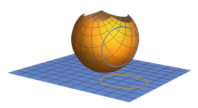
Task Space
Configuration Space
Alternatively: Over-Parametrziation
(e.g. Maximal Coordinates)
Thanks, Rebecca!
Thanks, Bernhard!
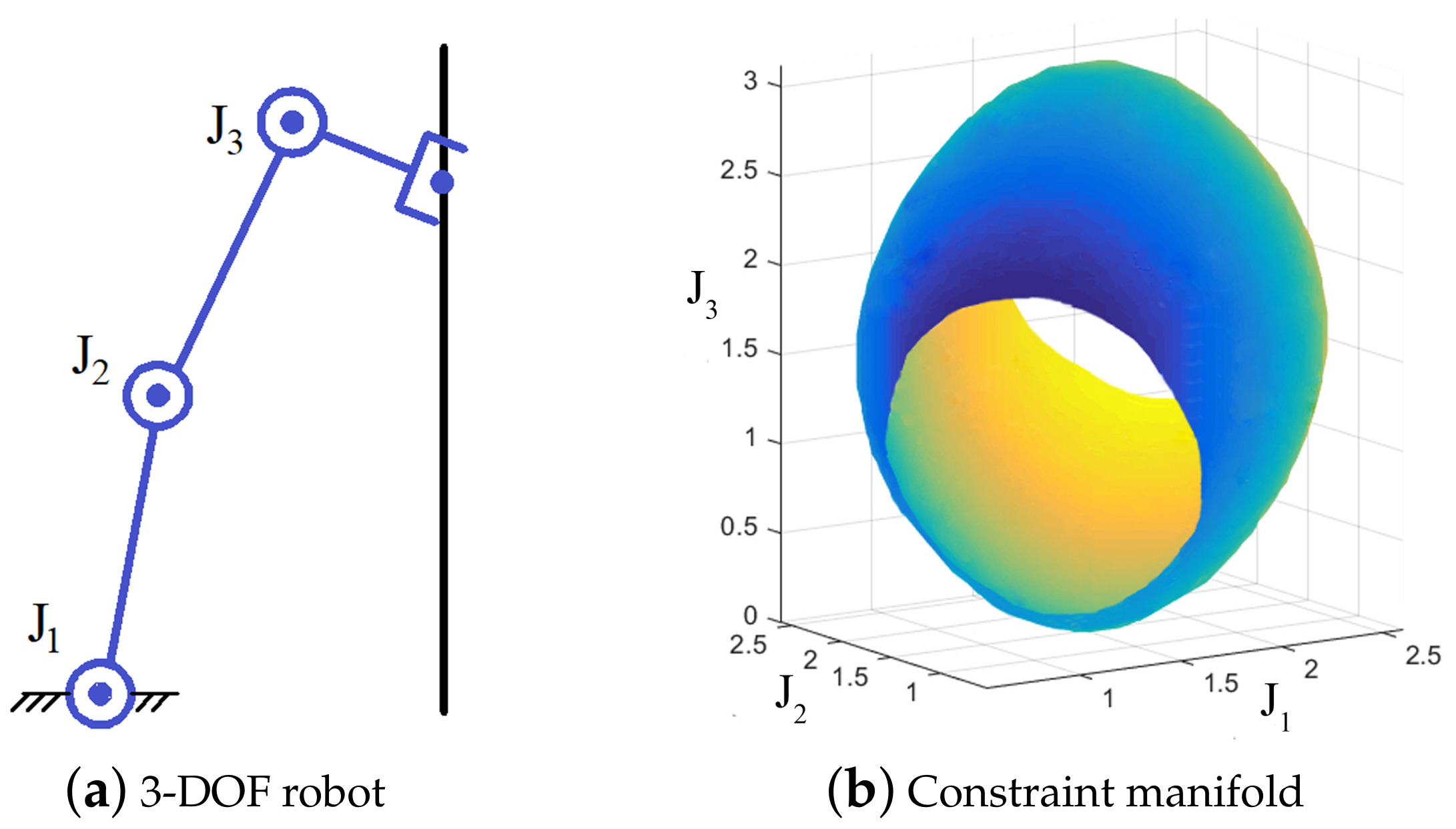
Task-Space Constraints
Learning the Metric of Task Constraint Manifolds for Constrained Motion Planning, Zha et. al.
Planning with Kinematic Constraints
Collision-Free Motion Planning Problem:
\[\begin{array}{rl}\min_\gamma & L(\gamma)\\ \operatorname{s.t.} & \gamma:[0,1]\to\mathbb R^n\\ & \gamma(0)=q_0,\gamma(1)=q_1\\ & g(\gamma(t))\le 0,\forall t\in[0,1]\end{array}\]
Constrained Collision-Free Motion Planning Problem:
\[\begin{array}{rl}\min_\gamma & L(\gamma)\\ \operatorname{s.t.} & \gamma:[0,1]\to\mathbb R^n\\ & \gamma(0)=q_0,\gamma(1)=q_1\\ & g(\gamma(t))\le 0,\forall t\in[0,1]\\ & h(\gamma(t))=0,\forall t\in[0,1]\end{array}\]
Existing Approaches
Sampling-Based Planning
Sampling-Based Methods for Motion Planning with Constraints, Kingston et. al.
Existing Approaches
Trajectory Optimization
Trajectory Optimization On Manifolds with
Applications to \(SO(3)\) and \(\mathbb{R}^3 \times S^2\), Watterson et. al.
Trajectory Optimization on Manifolds: A
Theoretically-Guaranteed Embedded Sequential
Convex Programming Approach, Bonalli et. al.
Direct Collocation Methods for Trajectory
Optimization in Constrained Robotic Systems, Bordabla et. al.
Our Idea: Plan with a Parametrization
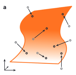
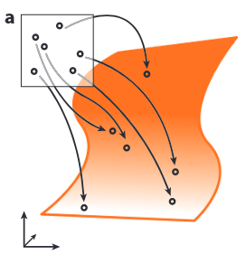
- Constraint manifold \(\mathcal M=\{q\in\mathbb R^n:h(q)=0\}\)
- Parametrization \(\xi:\mathcal U\to\mathbb R^n\) (with \(\mathcal U\subseteq\mathbb R^m\))
- Require:
- \(\xi\) is smooth and injective
- \(\xi(\mathcal U)\subseteq\mathcal M\), i.e., \(\forall \tilde q\in\mathcal U\), \(\xi(\tilde q)\in\mathcal M\)
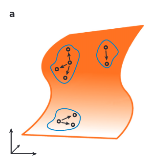
Parametrized Motion Planning Problem:
\[\begin{array}{rl}\min_{\tilde\gamma}& L(\xi\circ\tilde\gamma)\\ \operatorname{s.t.} & \tilde\gamma:[0,1]\to\mathcal U\\ & \tilde\gamma(0)=\tilde q_0,\tilde\gamma(1)=\tilde q_1\\ & g((\xi\circ\tilde\gamma)(t))\le 0,\forall t\in[0,1]\\ & h((\xi\circ\tilde\gamma)(t))=0,\forall t\in[0,1]\end{array}\]
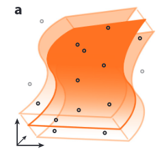
Intrinsic vs Extrinsic
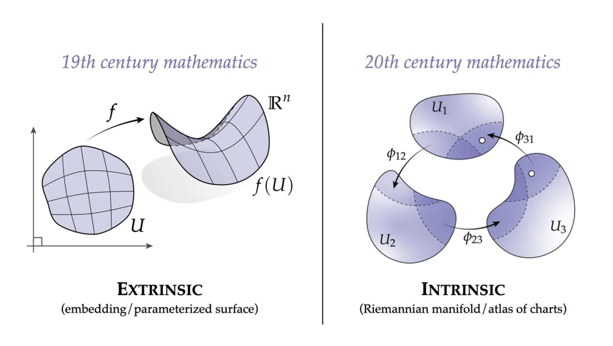
Keenan Crane (Twitter)
Building Parametrizations with Analytic IK
Analytic IK can be written as a function
\[\operatorname{IK}:\operatorname{SE}(3)\times\mathcal{C}\times\mathcal{D}\to\mathbb{R}^n,\]
where \(\mathcal{C}\) are continuous redundancy parameters and \(\mathcal{D}\) are discrete redundancy parameters.
By taking additional arguments, \(\operatorname{IK}\) is smooth and injective (almost everywhere). So we can build up parametrizations with it.
Parametrizing the Bimanual Constraint Manifold
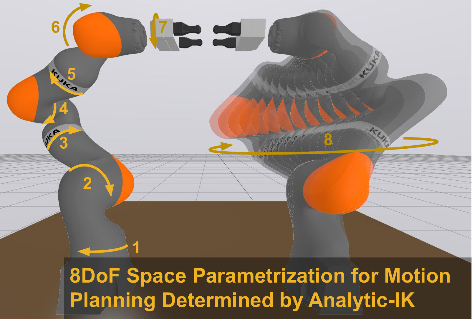
Alternative Parametrizations
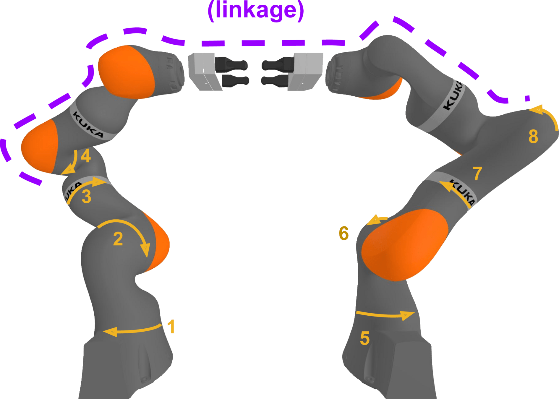
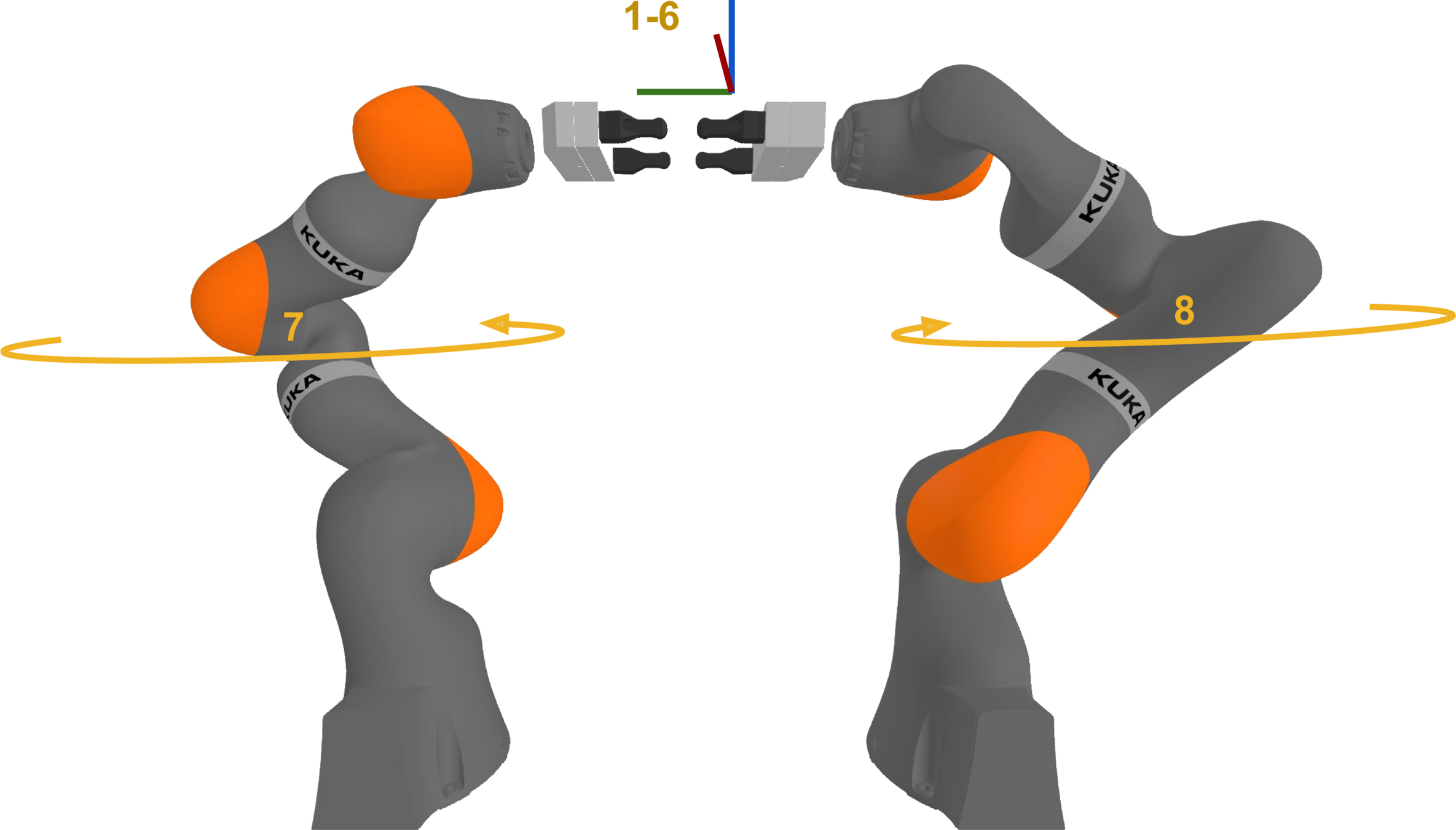
Key requirement: it has to be a minimal coordinate system
Planning with a Parametrization
Major effort to get the pieces needed into Drake
- Parametrization construction
- Domain validity constraints
- Region generation with IrisNp2 and IrisZo
(Full tutorial notebook releasing soon!)
Where are We Now?
Trajectory Optimization in Minimal Coordinates
Better Options for IK
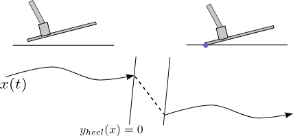
Crossing Between IK Branches
Setup: Just One Arm
How Can We Switch Branches?
For the KUKA iiwa, the branches meet when \(\theta_i\in\{0,\pi\}\) for \(i\in\{1,3,5\}\). Call this the coregular surface.
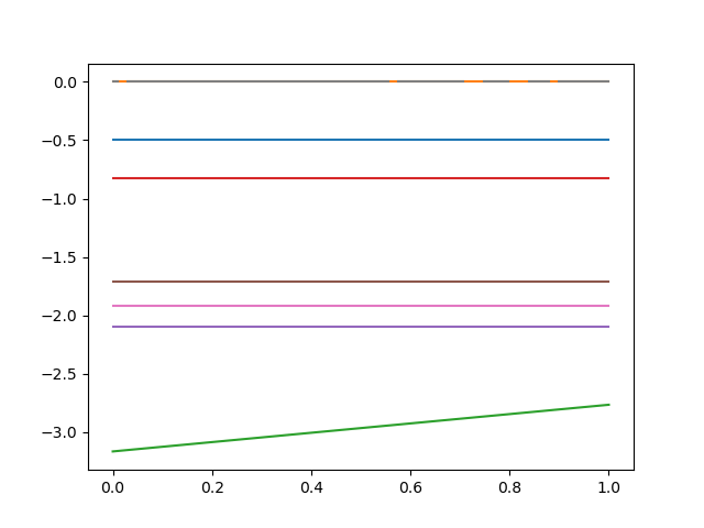
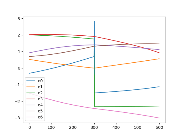
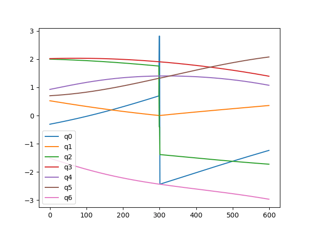
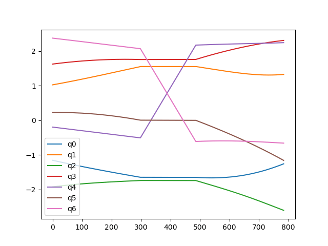
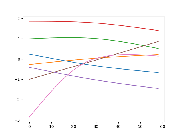
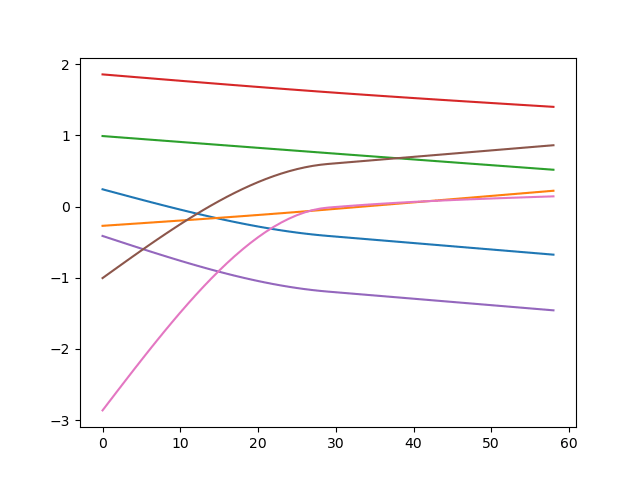
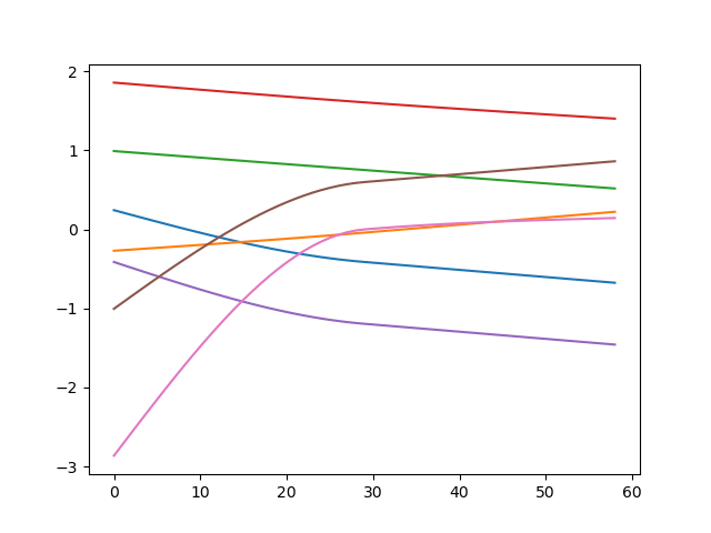
Here's a trajectory in joint space that crosses the coregular surface (x-axis is time):
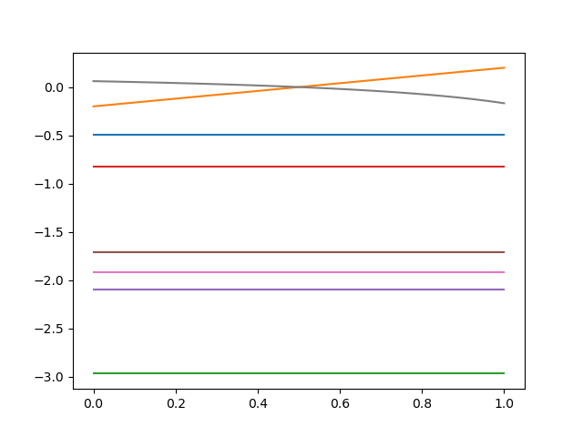
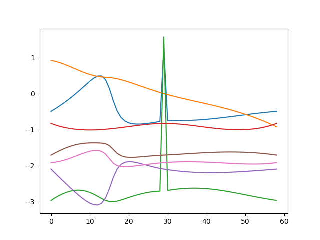
How Can We Switch Branches?
For the KUKA iiwa, the branches meet when \(\theta_i\in\{0,\pi\}\) for \(i\in\{1,3,5\}\). Call this the coregular surface.
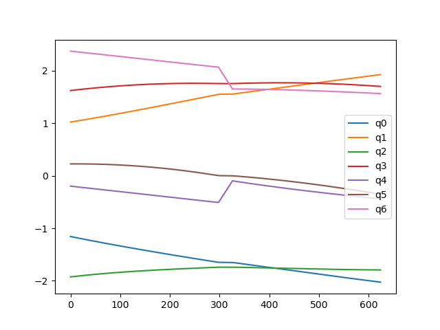
Now we can trace that trajectory in end-effector space, following two branches that should meet there.
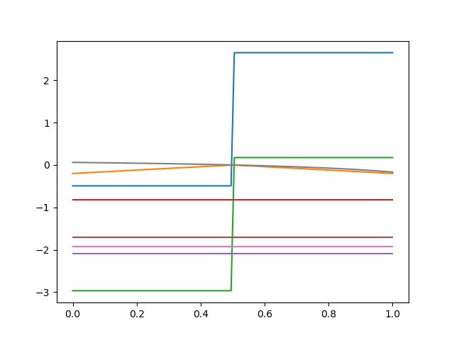
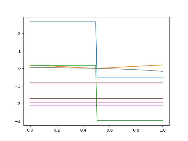
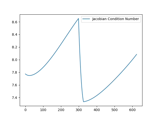
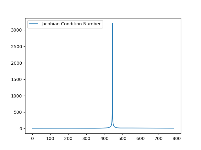
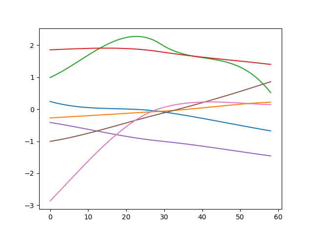
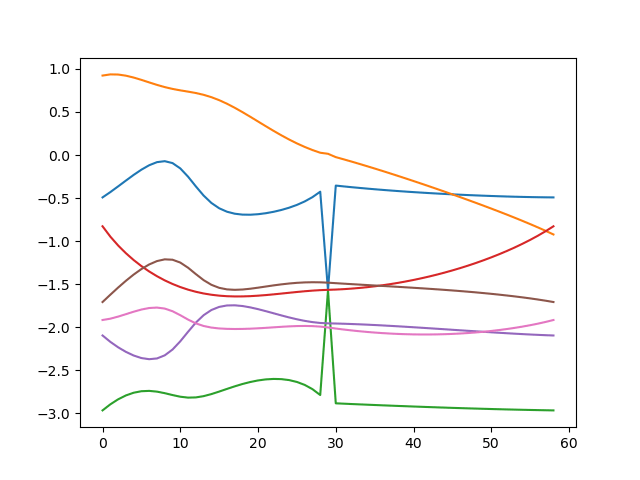
Moving along the Coregular Surface: Numerical Problems
Joint Space
Moving along the Coregular Surface: Numerical Problems

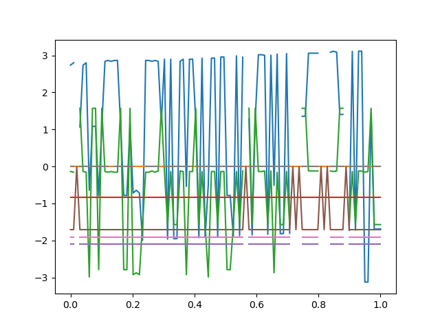
End-Effector Space
Self-Motion (Ordinarily)
Self-Motion (Near a Coregular Surface)
"Coregular" Self-Motion
"Coregular" Self-Motion
Singularities
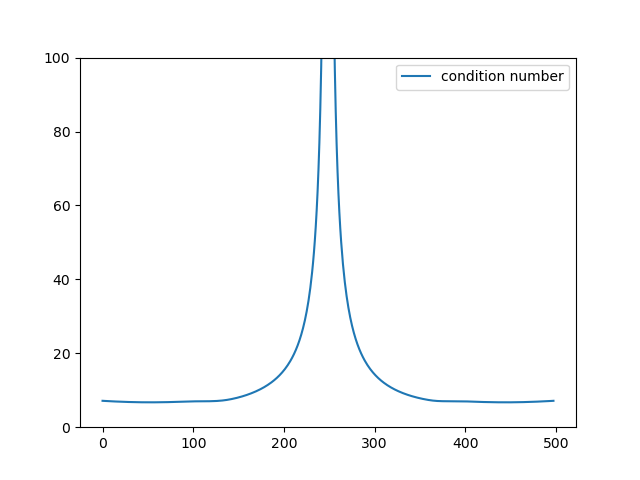
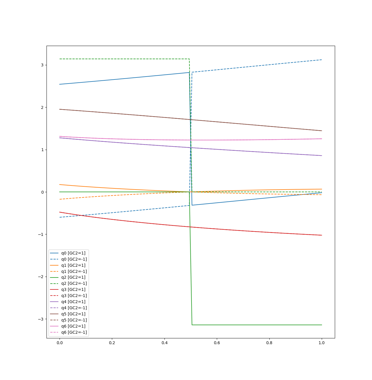
How Much Coregular Self-Motion?
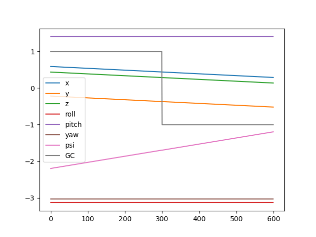
Examine the end-effector velocity into and out of the coregular point.
Parallel and flip the GC parameter?
\(\quad\rightarrow\) No coregular self-motion
Don't flip the GC parameter?
\(\quad\rightarrow\) \(180^\circ\) (max) coregular self-motion
Antiparallel and flip the GC parameter?
\(\quad\rightarrow\) \(180^\circ\) (max) coregular self-motion
Don't flip the GC parameter?
\(\quad\rightarrow\) No coregular self-motion
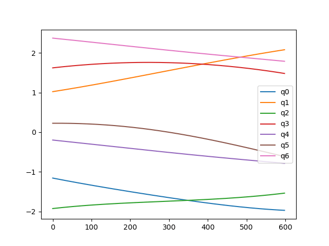
Example: No Flipping GC


Example: Flipping GC


Large vs Small Self-Motion
Best Option: Match Velocities?
Just need to handle the numerical issues
What Now?
Hybrid Trajectory Optimization
Model as a hybrid system (refer to Underactuated Ch.17)
- Modes are the branches of the IK function
- Guards detect the coregular surfaces
- Resets switch the IK branch, handle coregular self-motion, etc.
Underactuated Robotics, Tedrake
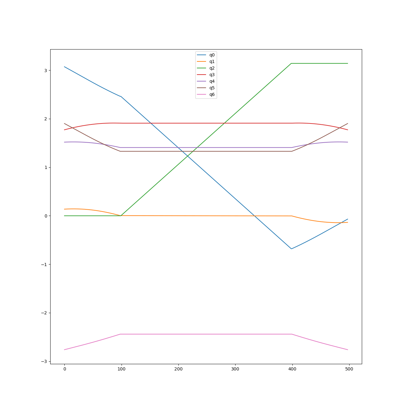
What If We Fix the Point?
End-Effector Trajectory
Joint Trajectory
Fixed Pose \(X_1(1)=X_2(0)=\hat X\)
Equal Velocity \(\dot X_1(1)=\dot X_2(0)\)
What if We Let the Point Move?
End-Effector Trajectory
Joint Trajectory
Equal Pose \(X_1(1)=X_2(0)\), "coregularity" \(\operatorname{IK}(X_1(1))_1=0\)
Equal Velocity \(\dot X_1(1)=\dot X_2(0)\)

Auxiliary Variable?
End-Effector Trajectory
Joint Trajectory
Equal Pose \(X_1(1)=X_2(0)=\operatorname{FK}(\bar q), \bar q_1=0\)
Equal Velocity \(\dot X_1(1)=\dot X_2(0)\)

Hack the Gradients?
Equal Pose \(X_1(1)=X_2(0)=\operatorname{FK}(\bar q), \bar q_1=0\)
Equal Velocity \(\dot X_1(1)=\dot X_2(0)\)
\(\left.\frac{d}{dt}\arccos(t)\right|_{t=1}:=\left.\frac{d}{dt}\right|\arccos(t)|_{t=0.9999}\)

What Now?
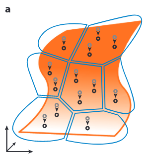
New Idea: An Atlas of IK Solutions
Maintain multiple parametrizations with different representational singularities
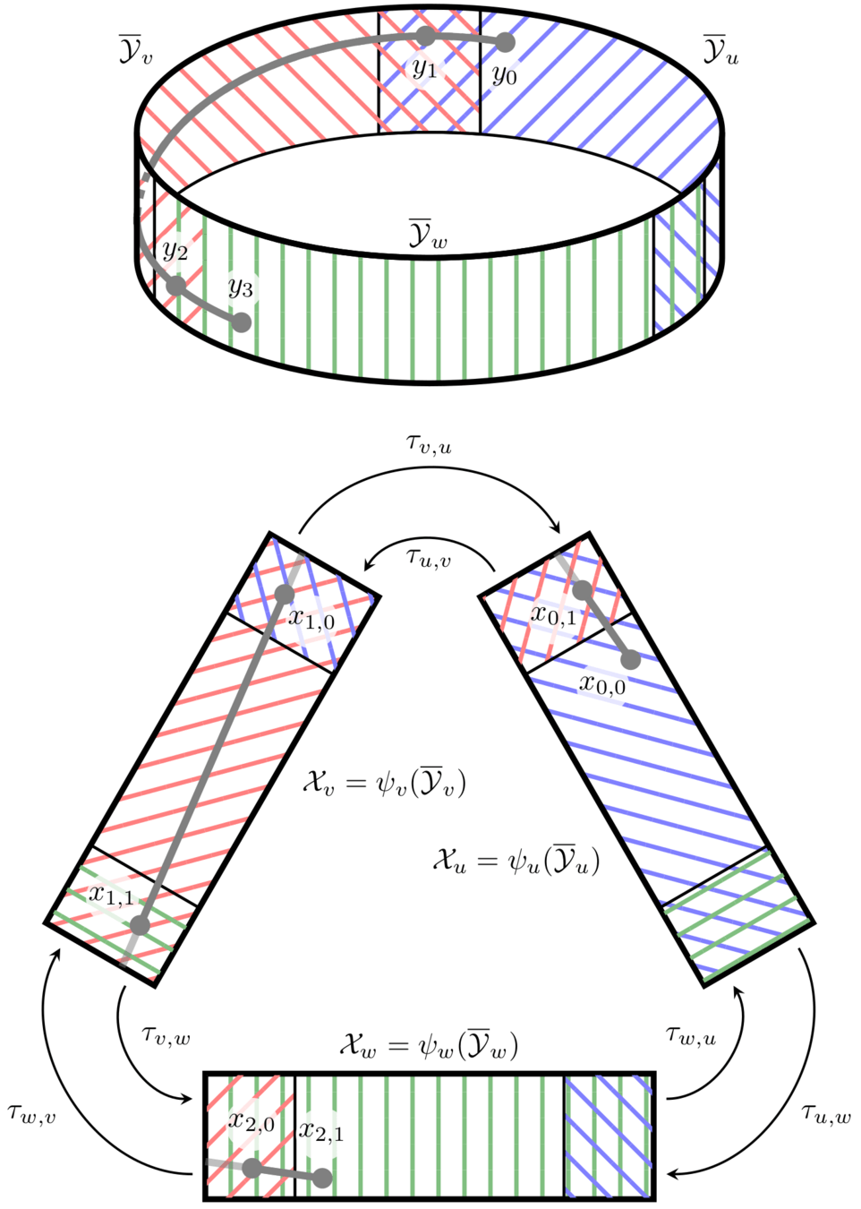
iiwa self-motion parametrizations:
- Shoulder-Elbow-Wrist
- First Joint
- Last Joint
This leads to more modes, but we can transition in their interior!
Trajectory Optimization in Minimal Coordinates for Kinematically-Constrained Systems
Thomas & Friends
November 21, 2025