Group Meeting Short Talk

Why should we care?

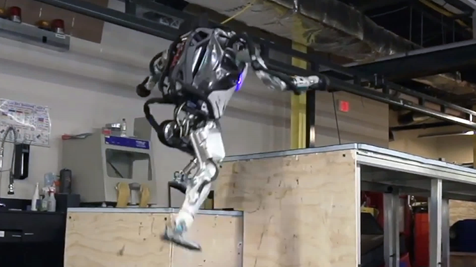
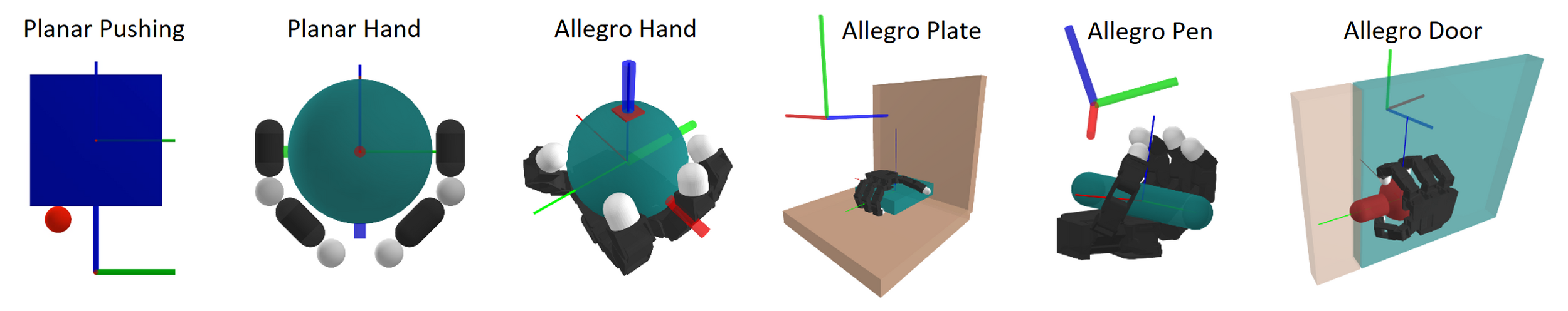
Agile & Autonomous Locomotion

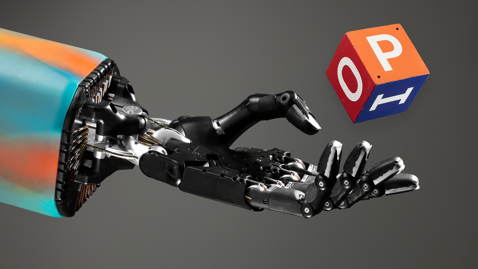
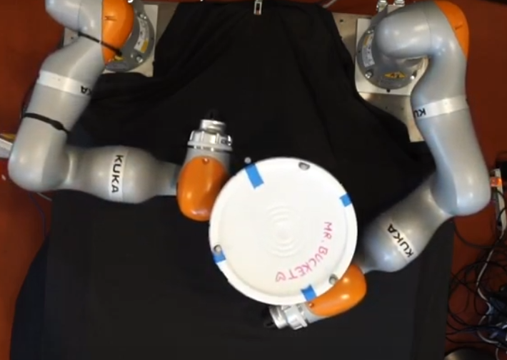
Dexterous Manipulation

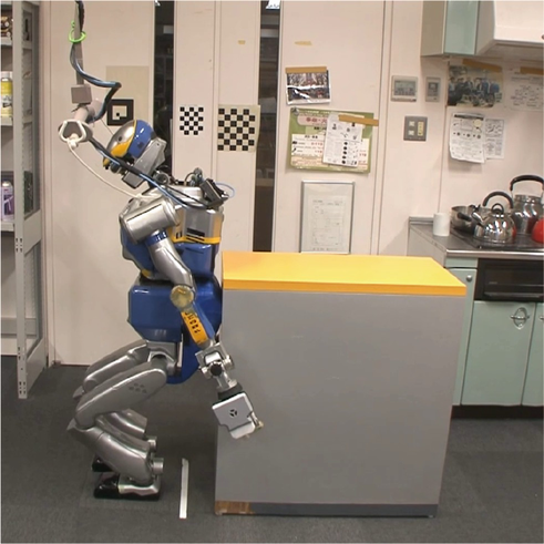
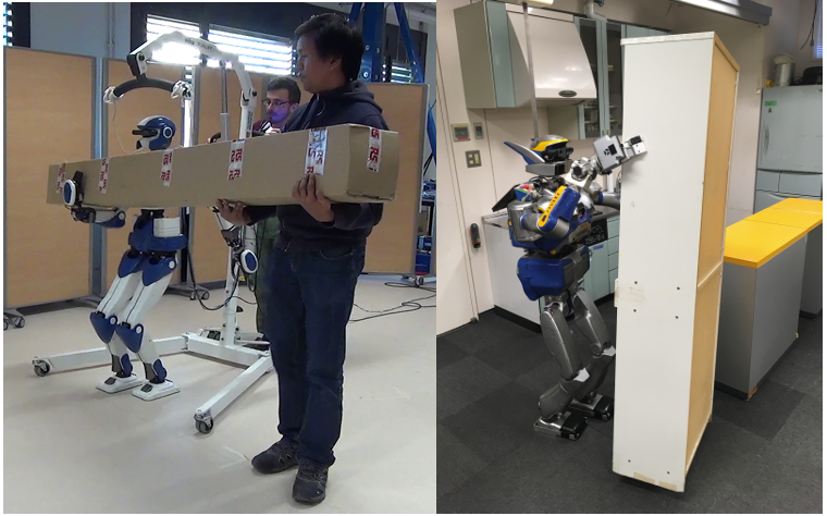
Whole-Body Loco-Manipulation

We still lack generalized solutions to all of these problems.

Why optimal control through contact?

Optimal Control Problem

\begin{aligned} \min_{\theta} & \; \bigg[V(\theta) \coloneqq c_T(x_T) + \sum^{T-1}_{t=0} \gamma^t c(x_t, u_t)\bigg] \\ \text{s.t.} & \; x_{t+1} = f(x_t, u_t) \\ & \; u_t = \pi(x_t, \theta) \end{aligned}

Cumulative Cost

Dynamics (Non-smooth)

Policy (can be open-loop)

Which class of problems are we dealing with today?

Optimization problems involving sequential decision making through non-smooth dynamics.

Action

State

Motivation: What makes this problem difficult?

The Non-Smooth Nature of Contact makes tools from smooth optimization difficult to use.

Making & Breaking Contact

Non-smoothness of Friction

Non-smoothness of Geometry

Today's Topic

1. How should we develop effective local feedback controllers for manipulation?

2. How can we attempt to overcome the locality of such approaches?

Inverse Dynamics as Local Control

\mathbf{M}(q)\ddot{q} + \mathbf{C}(q,\dot{q})\dot{q} + \mathbf{G}(q) = \tau + \sum_{i=1}^{n_c}\mathbf{J}^\top_i(q) \lambda_i

Forward Dynamics

Inverse Dynamics

q' = f(q,u)

u = f(q,q')

Inverse Dynamics Control

Given a desired acceleration of the robot, and the current state (joint state + velocities + contact forces), which torque should I apply to the robot?

Local Feedback Control: Inverse Dynamics

\mathbf{M}(q)\ddot{q} + \mathbf{C}(q,\dot{q})\dot{q} + \mathbf{G}(q) = \tau + \sum_{i=1}^{n_c}{\color{red} \mathbf{J}^\top_i(q)} \lambda_i

Inverse Dynamics Control for Smooth Systems

Given a desired acceleration of the robot, the current state, and the contact Jacobian (joint state + velocities), which torque should I apply to the robot?

Shortcomings

Only considers a fixed contact mode, and the controller no longer reasons about change of contact sequences during local control.

Okay for stabilizing locomotion (two feet are always on the ground), but spells trouble for manipulation!

How can we do better?

Shortcomings of Classical Inverse Dynamics Control

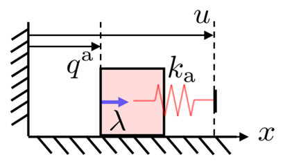
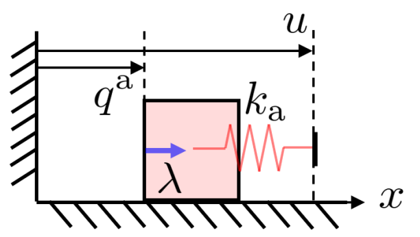
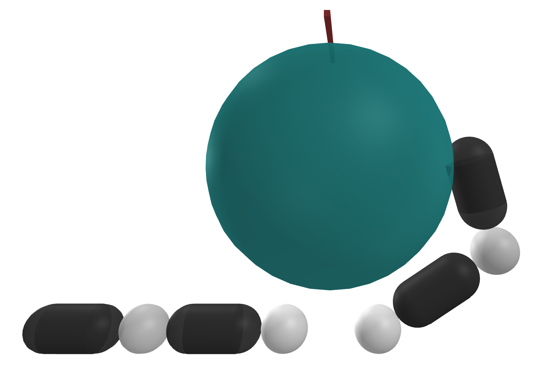
Background: Contact Dynamics

\begin{aligned} \text{find}\quad & \delta q^u, \delta q^a, \lambda_i \\ \text{s.t.}\quad & \mathbf{M}_u/h \delta q^u = \sum^{n_c}_{i=1} \mathbf{J}_{u_i}^\top \lambda_i \\ & h\mathbf{K}_a(q^a + \delta q^a - u) = \sum^{n_c}_{i=1} \mathbf{J}_{a_i}^\top \lambda_i \\ & \lambda_i \geq 0 \\ & \phi_i + \mathbf{J}_{a_i} \delta q^a + \mathbf{J}_{u_i} \delta q^u \geq 0 \\ & \lambda_i (\phi_i + \mathbf{J}_{a_i} \delta q^a + \mathbf{J}_{u_i} \delta q^u) = 0 \end{aligned}

Momentum-Impulse on Object

Impulse Balance on Robot Impedance

Contact Forces can only push, but not pull

Linearized Non-Penetration

Complementarity

q^a

q^u

u

\lambda

Actuated

Unactuated

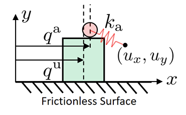
\begin{aligned} \text{find}\quad & \delta q^u, \delta q^a, \lambda_i \\ \text{s.t.}\quad & \mathbf{M}_u/h \delta q^u = \sum^{n_c}_{i=1} \mathbf{J}_{u_i}^\top \lambda_i \\ & h\mathbf{K}_a(q^a + \delta q^a - u) = \sum^{n_c}_{i=1} \mathbf{J}_{a_i}^\top \lambda_i \\ & \lambda_i \geq 0 \\ & \phi_i + \mathbf{J}_{a_i} \delta q^a + \mathbf{J}_{u_i} \delta q^u \geq 0 \\ & \lambda_i (\phi_i + \mathbf{J}_{a_i} \delta q^a + \mathbf{J}_{u_i} \delta q^u) = 0 \end{aligned}

Background: Contact Dynamics

\begin{aligned} \min_{\delta q^u,\delta q^a}\quad & \;\; \frac{1}{2} \delta {q^u}^\top \mathbf{M}/h \delta {q^u} + \frac{1}{2}\delta {q^a}^\top h\mathbf{K}_a \delta q^a - h\mathbf{K}_a (u - q^a) \delta q^a \\ \text{s.t.}\quad & \phi_i + \mathbf{J}_{a_i} \delta q^a + \mathbf{J}_{u_i} \delta q^u \geq 0 \quad \forall i\in \{1,\cdots,n_c\}\\ \end{aligned}

q^a

q^u

u

\lambda

\begin{aligned} \text{find}\quad & \delta q^u, \delta q^a, \lambda_i \\ \text{s.t.}\quad & \mathbf{M}_u/h \delta q^u = \sum^{n_c}_{i=1} \mathbf{J}_{u_i}^\top \lambda_i \\ & h\mathbf{K}_a(q^a + \delta q^a - u) = \sum^{n_c}_{i=1} \mathbf{J}_{a_i}^\top \lambda_i \\ & \lambda_i \geq 0 \\ & \phi_i + \mathbf{J}_{a_i} \delta q^a + \mathbf{J}_{u_i} \delta q^u \geq 0 \\ & \lambda_i (\phi_i + \mathbf{J}_{a_i} \delta q^a + \mathbf{J}_{u_i} \delta q^u) = 0 \end{aligned}

Dynamics Problem

Equivalent optimization problem

"Find me a minimum work configuration while respecting non-penetration."

Background Contact Dynamics

\begin{aligned} \min_{\delta q^a}\quad & \;\;\frac{1}{2}\delta {q^a}^\top h\mathbf{K}_a \delta q^a - h\mathbf{K}_a (u - q^a) \delta q^a \\ \text{s.t.}\quad & \phi_i + \delta q^a \geq 0 \quad \forall i\in \{1,\cdots,n_c\}\\ \end{aligned}

Optimal solution to the unconstrained problem:

\begin{aligned} \delta q^a = u - q^a \end{aligned}

Position command is exactly obeyed

\begin{aligned} q^a_\text{next} = q^a + \delta q^a = u \end{aligned}

If this solution meets constraints, then this is the optimal solution.

If not, optimality happens right at the boundary of the constraint.

\begin{aligned} u \end{aligned}

\begin{aligned} q^a_\text{next} \end{aligned}

Optimal Control with Contact Dynamics

\begin{aligned} \min_{u} \quad & \|q_\text{next} - q_g\|^2_\mathbf{Q} + \|u\|^2_\mathbf{R} \\ \text{s.t.} \quad & q_\text{next} = f(q, u) \\ \end{aligned}

What we care about is optimizing for some parameters of an optimal control problem.

We will take one-step trajectory optimization as an example.

But this is difficult because f describes an optimal solution to an optimization problem!

\begin{aligned} \min_{u} \quad & \|q_\text{next} - q_g\|^2_\mathbf{Q} + \|u\|^2_\mathbf{R} \\ \text{s.t.} \quad & q_\text{next} = q + \delta q^* \\ & \delta q^* = \text{arg}\min_{\delta q} \;\; g(\delta q,u) \;\; \text{s.t.} \;\; h(\delta q) \geq 0\\ \end{aligned}

Bi-level Optimization

Optimal Control with Contact Dynamics

KKT Reformulation Approach

Sensitivity Analysis Approach

\begin{aligned} \min_{u} \quad & \|q_\text{next} - q_g\|^2_\mathbf{Q} + \|u\|^2_\mathbf{R} \\ \text{s.t.} \quad & q_\text{next} = q + \delta q^* \\ & \delta q^* = \text{arg}\min_{\delta q} \;\; g(\delta q, u) \;\; \text{s.t.} \;\; h(\delta q) \geq 0\\ \end{aligned}

Bi-level Optimization

\begin{aligned} \min_{u, \lambda, \delta q} \quad & \|q_\text{next} - q_g\|^2_\mathbf{Q} + \|u\|^2_\mathbf{R} \\ \text{s.t.} \quad & q_\text{next} = q + \delta q^* \\ & \nabla_{\delta q} g(\delta q) - \lambda^\top \nabla_{\delta q} h(\delta q) = 0 \\ & h(\delta q) \geq 0\\ & \lambda \geq 0 \\ & h(\delta q)\lambda = 0 \end{aligned}

Two approaches to tackling these in general.

Solvers hate the nonconvexity from complementarity.

Two approaches to tackling these in general.

If we have the gradients

\begin{aligned} \frac{\partial \delta q^*}{\partial u} \end{aligned}

through sensitivity analysis of the inner optimization problem, then possible to plug this into iterative solvers.

Sensitivity Analysis

What do gradients do? They allow us to construct a locally linear model around the current iterate.

\begin{aligned} \min_{u} \quad & \|q_\text{next} - q_g\|^2_\mathbf{Q} + \|u\|^2_\mathbf{R} \\ \text{s.t.} \quad & q_\text{next} = \mathbf{B}(q,\bar{u})(u - \bar{u}) + f(q,\bar{u}) \\ \end{aligned}

We had used this sensitivity extensively in previous projects.

\begin{aligned} \mathbf{B}(q,\bar{u}) = \frac{\partial q_\text{next}(q,u)}{\partial u}\bigg|_{q=q,u=\bar{u}} \end{aligned}

1. This is a linearization of the dynamics, allows us to tools such as iLQR.

2. Linearization also allows us to approximate reachability effectively.

Inverse Dynamics Interpretation

If we strictly enforce the goal displacement, we obtain inverse dynamics from locomotion.

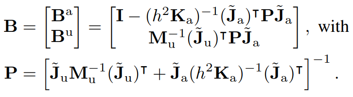
\begin{aligned} \min_{u} \quad & \|u\|^2_\mathbf{R} \\ \text{s.t.} \quad & q_\text{next} = q_g \\ & q_\text{next} = \mathbf{B}(q,\bar{u})(u - \bar{u}) + f(q,\bar{u}) \\ \end{aligned}

\begin{aligned} \mathbf{B}(q,\bar{u}) = \frac{\partial q_\text{next}(q,u)}{\partial u}\bigg|_{q=q,u=\bar{u}} \end{aligned}

Note that B is highly abstracted out here, but actually corresponds to a lot of Jacobian computations.

It answers queries of "if I think of active contacts as a joint, how does my actuator torques affect forces onto the configuration of the object locally?"

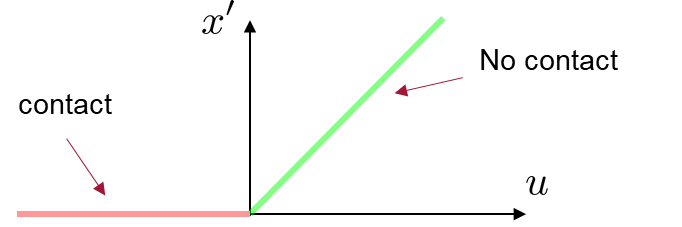
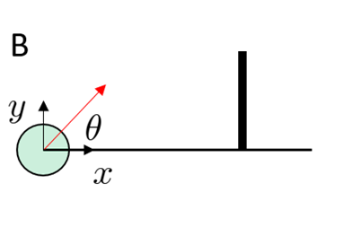
\begin{aligned} \min_{u} \quad & \|q^u_\text{next} - q^u_g\|^2_\mathbf{Q} \\ \text{s.t.} \quad & q^u_\text{next} = \mathbf{B}^u(q,\bar{u})(u - \bar{u}) + f^u(q,\bar{u}) \\ & |u - \bar{u}| \leq \varepsilon\mathbf{1} \end{aligned}

Shortcomings of Linearization

\begin{aligned} u \end{aligned}

\begin{aligned} q^u_\text{next} \end{aligned}

q^u

q^a

u

\lambda

\begin{aligned} q^u_g \end{aligned}

Current position

\begin{aligned} q^a \end{aligned}

No Gradient information!

If the object is not in contact, traditional inverse dynamics is not effective.

Fortunately, smoothing comes to the rescue.

\begin{aligned} \min_{u} \quad & \|q^u_\text{next} - q^u_g\|^2_\mathbf{Q} \\ \text{s.t.} \quad & q^u_\text{next} = {\color{red}\mathbf{B}^u_\rho}(q,\bar{u})(u - \bar{u}) + {\color{red}f^u_\rho}(q,\bar{u}) \\ & |u - \bar{u}| \leq \varepsilon\mathbf{1} \end{aligned}

q^u

q^a

u

\lambda

rho subscript denotes smoothing

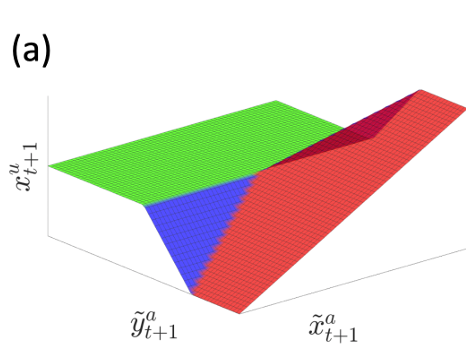
Shortcomings of Linearization

0.5m

0.0m

We have linearized the smoothened dynamics around u = qa.

Depending on where we set the goal to be, we see three distinct regions.

\begin{aligned} \min_{u} \quad & \|q^u_\text{next} - q^u_g\|^2_\mathbf{Q} \\ \text{s.t.} \quad & q^u_\text{next} = {\color{red}\mathbf{B}^u_\rho}(q,\bar{u})(u - \bar{u}) + {\color{red}f^u_\rho}(q,\bar{u}) \\ & |u - \bar{u}| \leq \varepsilon\mathbf{1} \end{aligned}

q^u

q^a

u

\lambda

rho subscript denotes smoothing

Shortcomings of Linearization

0.5m

0.0m

Region 1. Beneficial Bias

Goal = 0.61m

Optimal input

The linearized model provides helpful bias, as the optimal input moves the actuated body towards making contact.

\begin{aligned} \min_{u} \quad & \|q^u_\text{next} - q^u_g\|^2_\mathbf{Q} \\ \text{s.t.} \quad & q^u_\text{next} = {\color{red}\mathbf{B}^u_\rho}(q,\bar{u})(u - \bar{u}) + {\color{red}f^u_\rho}(q,\bar{u}) \\ & |u - \bar{u}| \leq \varepsilon\mathbf{1} \end{aligned}

q^u

q^a

u

\lambda

rho subscript denotes smoothing

Shortcomings of Linearization

0.5m

0.0m

Region 2. Hurtful Bias

Goal = 0.52m

Optimal input

If you command the actuated body to hold position, the unactuated body will be pushed away due to smoothing.

The actuated body wants to go backwards in order to decrease this effect if the goal is not too in front of the unactuated body.

\begin{aligned} \min_{u} \quad & \|q^u_\text{next} - q^u_g\|^2_\mathbf{Q} \\ \text{s.t.} \quad & q^u_\text{next} = {\color{red}\mathbf{B}^u_\rho}(q,\bar{u})(u - \bar{u}) + {\color{red}f^u_\rho}(q,\bar{u}) \\ & |u - \bar{u}| \leq \varepsilon\mathbf{1} \end{aligned}

q^u

q^a

u

\lambda

rho subscript denotes smoothing

Shortcomings of Linearization

0.5m

0.0m

Region 3. Violation of unilateral contact

Goal = 0.45m

Optimal input

If you set the goal to behind the unactuated body, the linear model thinks that it can pull, and will move backwards.

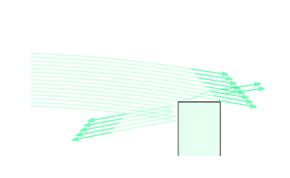
Reachable Set Computation

\begin{aligned} q^u_g \end{aligned}

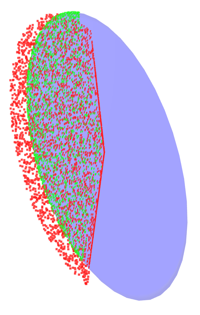
Simulator rollouts of a action norm-ball

Ellipsoid informed by the local B matrix

Similarly, we are horribly off in our approximation of the reachable set constructed from the B matrix.

Clearly we need to think about forces in order to property define reachable sets under linearization

But we don't have contact forces as a decision variable...how?

Linearizing an Optimal Solution

\begin{aligned} \min_x \quad & x^\intercal \mathbf{Q} x + b(\theta)^\intercal x \\ \quad & \mathbf{A}x \leq b \end{aligned}

What does it mean to create a locally linear model of a solution of an optimization problem?

\begin{aligned} x(\theta) & = x^*(\bar{\theta}) + \mathbf{J}(\bar{\theta})(\theta - \bar{\theta}) \\ \end{aligned}

Generic QP

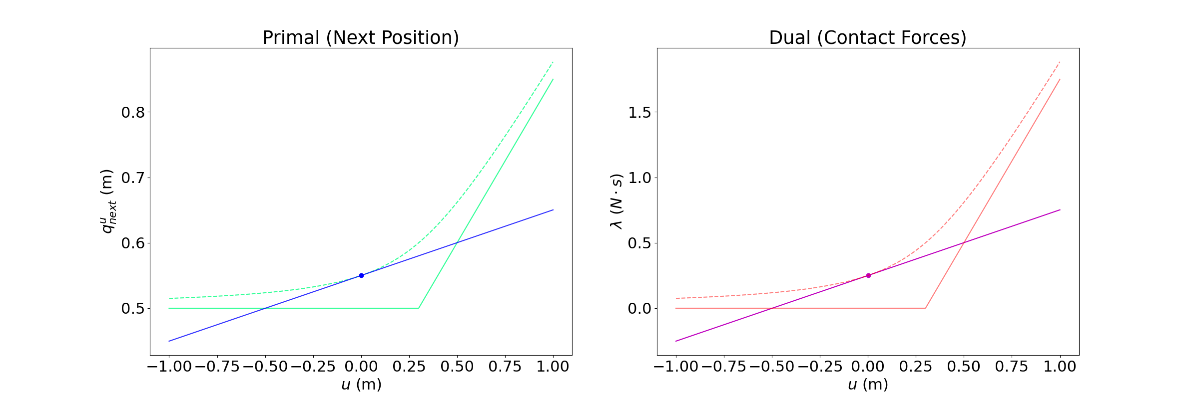
Linear Model of Primal solution vs. Parameters

\begin{aligned} \mathbf{J}(\bar{\theta})\coloneqq \frac{\partial \delta q^*(\theta)}{\partial \theta}\bigg|_{\theta=\bar{\theta}} \end{aligned}

Linearizing an Optimal Solution

\begin{aligned} \min_x \quad & x^\intercal \mathbf{Q} x + b(\theta)^\intercal x \\ \quad & \mathbf{A}x \leq b \end{aligned}

What does it mean to create a locally linear model for an optimization problem?

\begin{aligned} x(\theta) & = x^*(\bar{\theta}) + \mathbf{J}(\bar{\theta})(\theta - \bar{\theta}) \\ \end{aligned}

Generic QP

Linear Model of Primal solution vs. Parameters

\begin{aligned} \mathbf{J}(\bar{\theta})\coloneqq \frac{\partial x^*(\theta)}{\partial \theta}\bigg|_{\theta=\bar{\theta}} \end{aligned}

Linear Model of Dual solution vs. Parameters

\begin{aligned} \lambda(\theta) & = \lambda^*(\bar{\theta}) + \mathbf{\Lambda}(\bar{\theta})(\theta - \bar{\theta}) \\ \end{aligned}

\begin{aligned} \mathbf{\Lambda}(\bar{\theta})\coloneqq \frac{\partial \lambda^*(\theta)}{\partial \theta}\bigg|_{\theta=\bar{\theta}} \end{aligned}

We can enforce primal and dual feasibility as the domain of the linear model.

\begin{aligned} \mathcal{D} \coloneqq \{\theta | \lambda(\theta)\geq 0, Ax(\theta) \leq b\} \end{aligned}

New Approach at Linearization

Linearizing the dual and forcing the linear model of the dual to be positive discards the unilateral violation region.

New Approach at Linearization

Interestingly, one solution to getting rid of the hurtful bias region is to keep the slope of the linearization, but make it pass through the non-smooth dynamics.

(e.g. keep the direction, but respect the fact that if no contact will result in no movement)

Applications

- is not limited to limit surfaces ;)

- accounts for non-fixed contact modes

- respects unilateral contact

Inverse Dynamics on Optimization-based Dynamics

Proper Generalization of a Motion Cone

\begin{aligned} \min_{u, \lambda_i} \quad & \|q^u_\text{next} - q^u_g\|^2_\mathbf{Q} \\ \text{s.t.} \quad & q^u_\text{next} = \mathbf{B}^u_\rho(\bar{q},\bar{u})(u - \bar{u}) + f^u(\bar{q},\bar{u}) \\ & \lambda_i = \mathbf{\Lambda}_\rho(\bar{q},\bar{u})(\lambda - \bar{\lambda}) + \lambda(\bar{q},\bar{u}) \\ & \lambda_i \geq 0 \\ & |u - \bar{u}| \leq \varepsilon\mathbf{1} \end{aligned}

Key Takeaway

Whenever someone linearizes optimization-based dynamics, ask them if they've considered their domains for dual feasibility :)

Goals of the Internship

1. How should we develop effective local feedback controllers for manipulation?

2. How can we attempt to overcome the locality of such approaches?

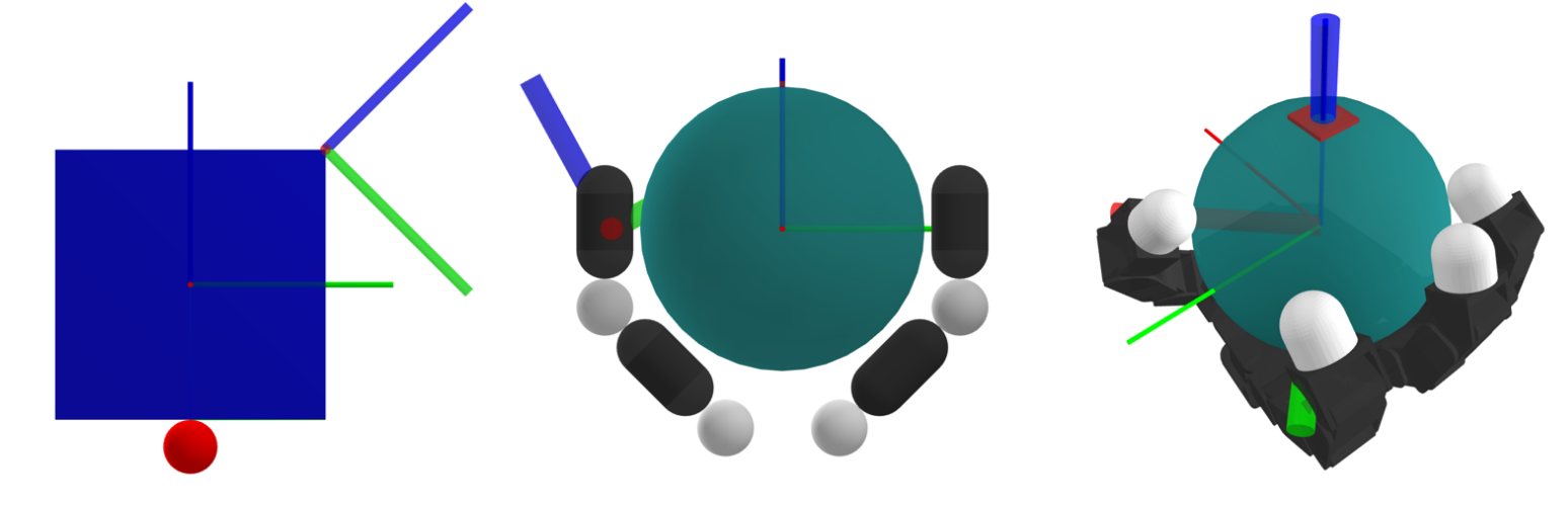
Regrasping as an Action Space

Finger Gaiting as an example of non-local control

We rotate our fingers up until we reach joint limits, then travel to the other end of the joint limit.
In the space of joint torques, a highly non-trivial / non-local action! (Required action betrays direction of local improvement)

Asking for more from an MPC-based controller seems fundamentally limiting due to non-trivial local minima.

Maybe we're asking the wrong thing from our optimization problems?

Actuator Relocation

If you had the choice of placing your actuator anywhere, where would you place it?

Actuator Relocation

If you had the choice of placing your actuator anywhere, where would you place it?

Did you reason about the fine-grained path of how you got there?

Mathematical Formulation

\begin{aligned} \min_{u, \lambda_i} \quad & \|q^u_\text{next} - q^u_g\|^2_\mathbf{Q} + \|u\|^2_\mathbf{R}\\ \text{s.t.} \quad & q^u_\text{next} = \mathbf{B}^u_\rho(\bar{q},\bar{u})(u - \bar{u}) + f^u(\bar{q},\bar{u}) \\ & \lambda_i = \mathbf{\Lambda}_\rho(\bar{q},\bar{u})(\lambda - \bar{\lambda}) + \lambda(\bar{q},\bar{u}) \\ & \lambda_i \geq 0 \\ \end{aligned}

Inverse Dynamics Controller

\begin{aligned} \min_{u, \lambda_i, {\color{red}\bar{q}^a}} \quad & \|q^u_\text{next} - q^u_g\|^2_\mathbf{Q} + \|u\|^2_\mathbf{R}\\ \text{s.t.} \quad & q^u_\text{next} = \mathbf{B}^u_\rho(\bar{q}^u,{\color{red}\bar{q}^a},\bar{u})(u - \bar{u}) + f^u(\bar{q}^u,{\color{red}\bar{q}^a},\bar{u}) \\ & \lambda_i = \mathbf{\Lambda}_\rho(\bar{q}^u, {\color{red}\bar{q}^a},\bar{u})(\lambda - \bar{\lambda}) + \lambda(\bar{q}^u,{\color{red}\bar{q}^a},\bar{u}) \\ & \lambda_i \geq 0 \\ & {\color{red} \phi(\bar{q}^u,{\color{red} \bar{q}^a}) \geq 0 } \end{aligned}

Contact Sampling

QP / SOCP

Highly Nonlinear /

More Global Problem!

Current Status: Sample

Non-penetration

Current Ongoing Research

\begin{aligned} \min_{u, \lambda_i, {\color{red}\bar{q}^a}} \quad & \|q^u_\text{next} - q^u_g\|^2_\mathbf{Q} + \|u\|^2_\mathbf{R}\\ \text{s.t.} \quad & q^u_\text{next} = \mathbf{B}^u_\rho(\bar{q}^u,{\color{red}\bar{q}^a},\bar{u})(u - \bar{u}) + f^u(\bar{q}^u,{\color{red}\bar{q}^a},\bar{u}) \\ & \lambda_i = \mathbf{\Lambda}_\rho(\bar{q}^u, {\color{red}\bar{q}^a},\bar{u})(\lambda - \bar{\lambda}) + \lambda(\bar{q}^u,{\color{red}\bar{q}^a},\bar{u}) \\ & \lambda_i \geq 0 \\ & {\color{red} \phi(\bar{q}^u,{\color{red} \bar{q}^a}) \geq 0 } \end{aligned}

Contact Sampling

How do we solve this problem more efficiently?

- Gradient-based methods

Non-penetration

Do we have the right objective?

Inverse Dynamics Control for Optimization-Based Dynamics