Motion Sets for Contact-Rich Manipulation
What is sensitivity analysis really?
Consider a simple QP, we want the gradient of optimal solution w.r.t. parameters,
and it's KKT conditions
As we perturb q, the optimal solution changes to preserve the equality constraints in KKT.
What is sensitivity analysis really?
Consider a simple QP, we want the gradient of optimal solution w.r.t. parameters,
and it's KKT conditions
Differentiate the Equalities w.r.t. q

What is sensitivity analysis really?
Consider a simple QP, we want the gradient of optimal solution w.r.t. parameters,
and it's KKT conditions
Throw away inactive constraints and linsolve.
Limitations of Sensitivity Analysis
1. Throws away inactive constraints
2. Throws away feasibility constraints
Gradients are "correct" but too local!
Remedy 1. Constraint Smoothing
1. Throws away inactive constraints
2. Throws away feasibility constraints
Gradients are "correct" but too local!
Numerous benefits to smoothing that we already know so far
But doesn't address the second issue with feasibility!
For most solvers, feasibility has to be handled with line search.
Remedy 2. Handling Inequalities
Connection between gradients and "best linear model" still generalizes.
What's the best linear model that locally approximates xstar as a function of q?
Remedy 2. Handling Inequalities
Connection between gradients and "best linear model" still generalizes.
What's the best linear model that locally approximates xstar as a function of q?
IF we didn't have feasibility constraints, the answer is Taylor expansion
Connection between gradients and "best linear model" still generalizes.
What's the best linear model that locally approximates xstar as a function of q?
But not every direction of dq results in feasibility!
KKT Conditions
Remedy 2. Handling Inequalities
Linearize the Inequalities to limit directions dq.
KKT Conditions
Set of locally "admissible" dq.
Remedy 2. Handling Inequalities
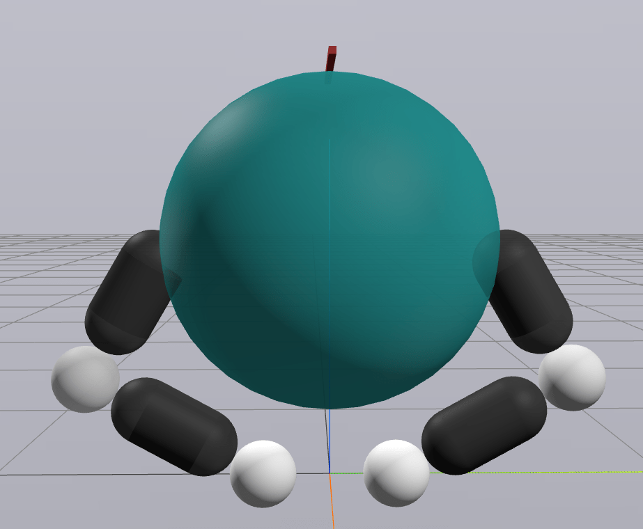
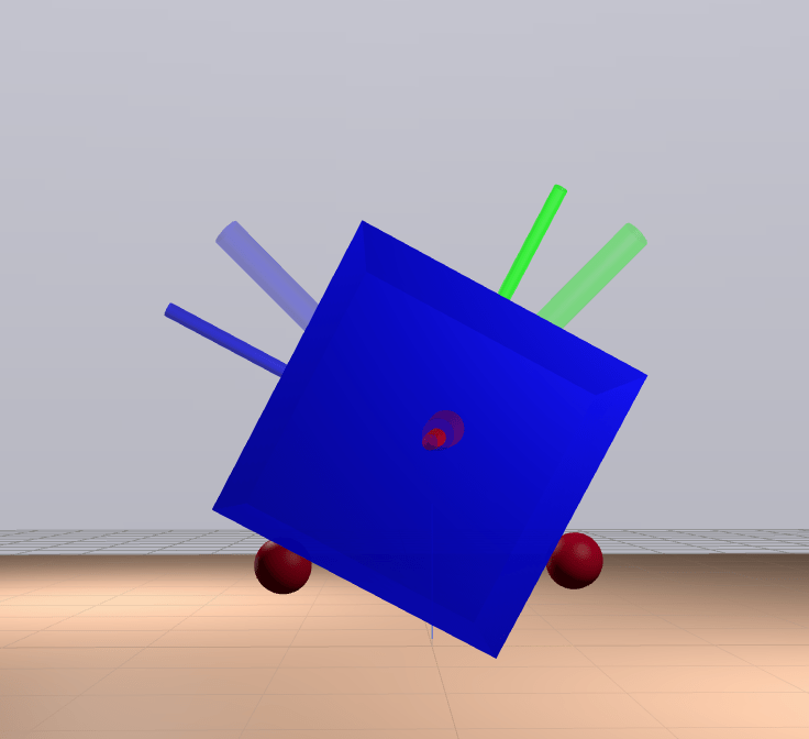
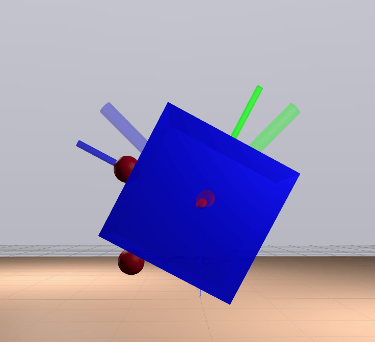
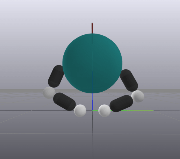
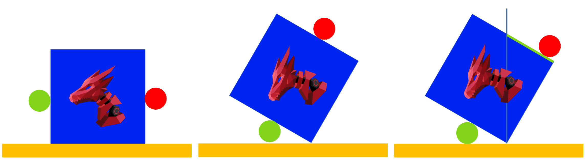
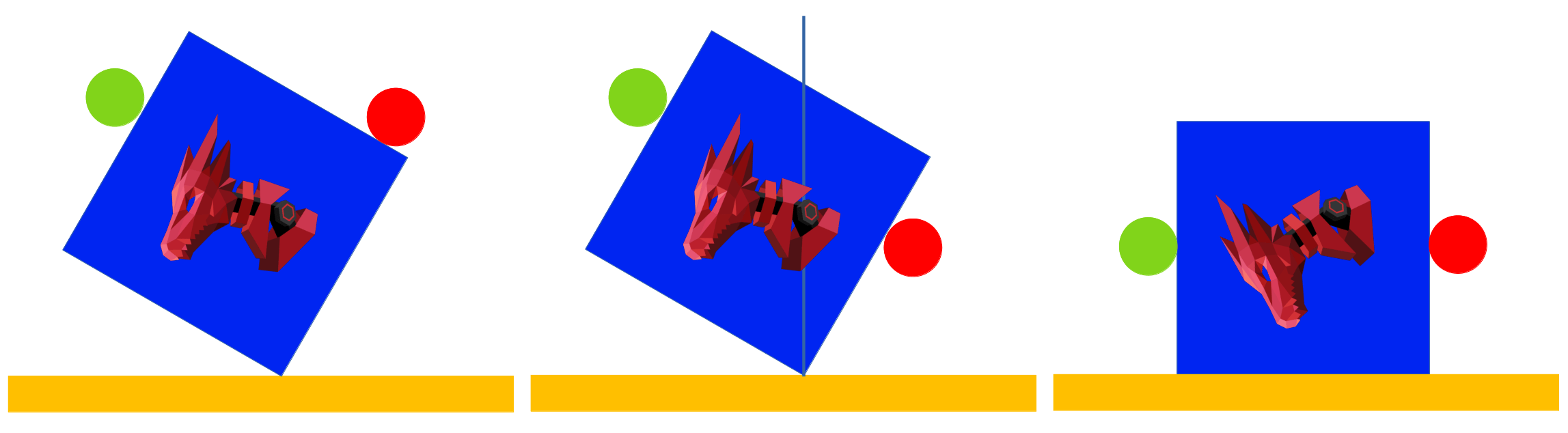
Wrench Set
Recall the "Wrench Set" from old grasping literature.
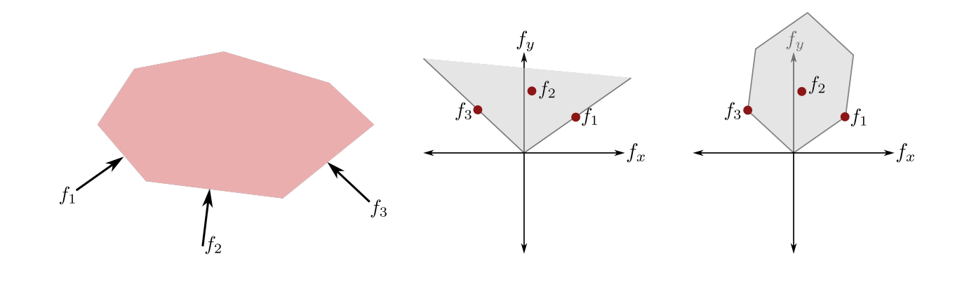
from Stanford CS237b
Recall the "Wrench Set" from old grasping literature.
Under quasistatic dynamics, the movement of the object is a linear transform of this wrench set.
Wrench Set
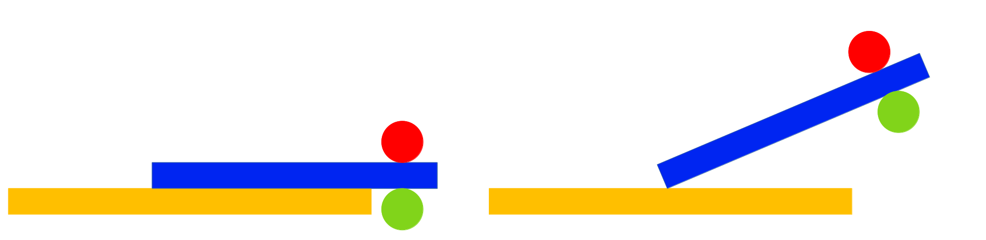
Wrench Set: Limitations
Recall the "Wrench Set" from old grasping literature.
Under quasistatic dynamics, the movement of the object is a linear transform of this wrench set.
But the wrench set has limitations if we go beyond point fingers
1. Singular configurations of the manipulator
2. Self collisions within the manipulator
3. Joint Limits of the manipulator
4. Torque limits of the manipulator
The Achievable Wrench Set
Write down forces as function of input instead
Recall the "Wrench Set" from old grasping literature.
The Achievable Wrench Set
Write down forces as function of input instead
Recall the "Wrench Set" from old grasping literature.
Recall we also have linear models for these forces!
The Achievable Wrench Set
Let's compute the Jacobian sum
The Achievable Wrench Set
Let's compute the Jacobian sum
Transform it to generalized coordinates
The Achievable Wrench Set
Let's compute the Jacobian sum
Transform it to generalized coordinates
The Achievable Wrench Set
Transform it to generalized coordinates
To see the latter term, note that from sensitivity analysis,
The Achievable Wrench Set
Transform it to generalized coordinates
This is the B matrix for iLQR, inverse dynamics, etc.
that differentiable simulators give
The Achievable Wrench Set
Transform it to generalized coordinates
This is the B matrix for iLQR, inverse dynamics, etc.
that differentiable simulators give
But what happened to the constraints?
The Achievable Wrench Set
Transform it to generalized coordinates
Need to add these back in through model of dual variables
Trust Region Interpretation
Transform it to generalized coordinates
Need to add these back in through model of dual variables
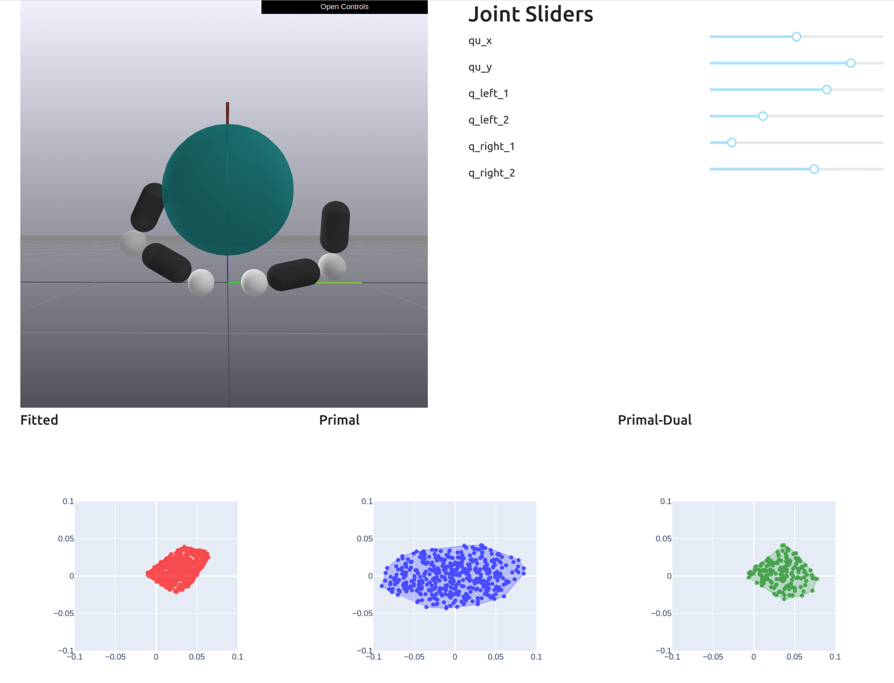
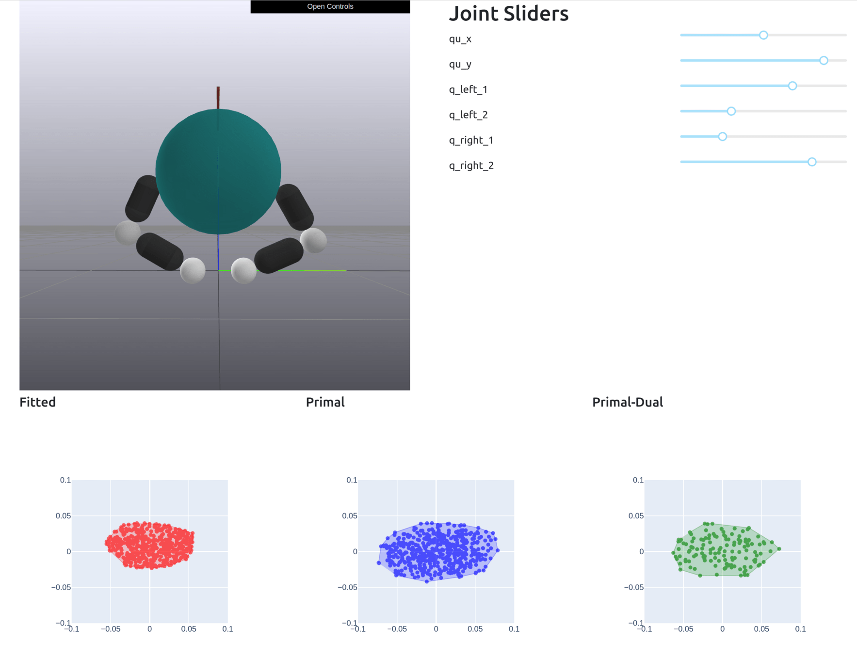
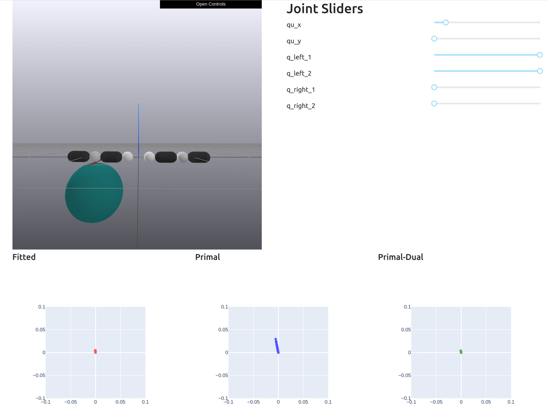
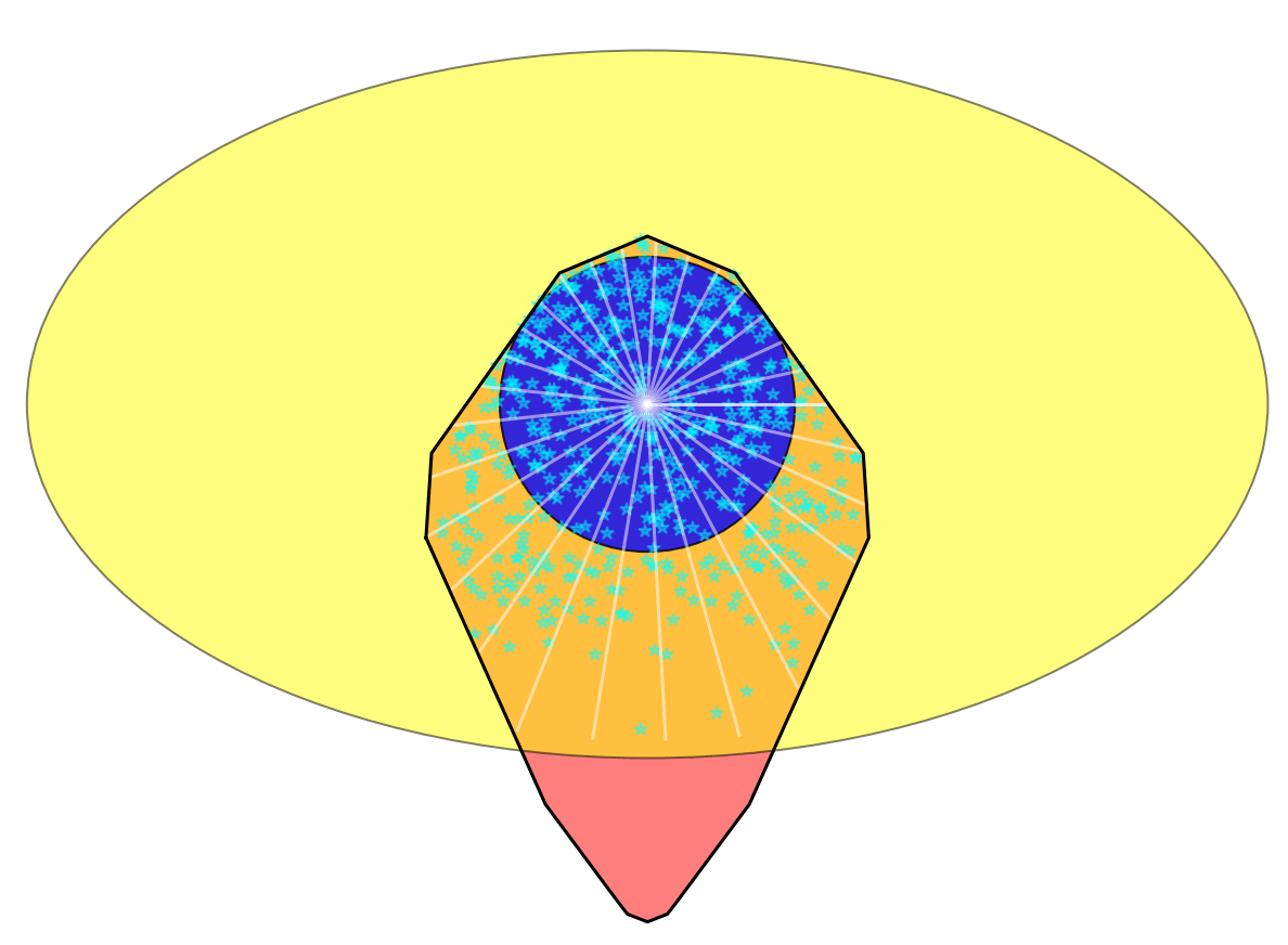
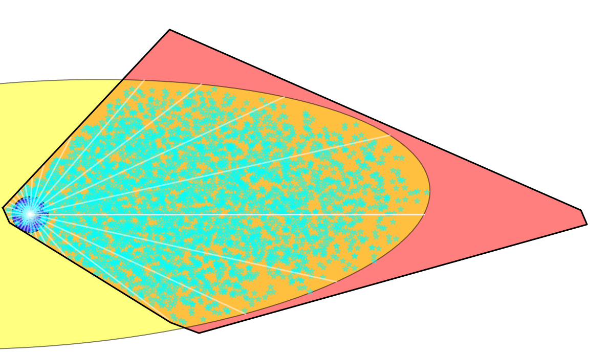
Formally Defining Motion Set
Given , solve the dynamics to obtain the Motion Set parameters.
Define the Motion Set as
+ additional constraints (joint limit, torque limit)
Formally Defining Motion Set
Given , solve the dynamics to obtain the Motion Set parameters.
Define the Motion Set as
+ additional constraints (joint limit, torque limit)
This set is always convex

Folk Physics for Apes
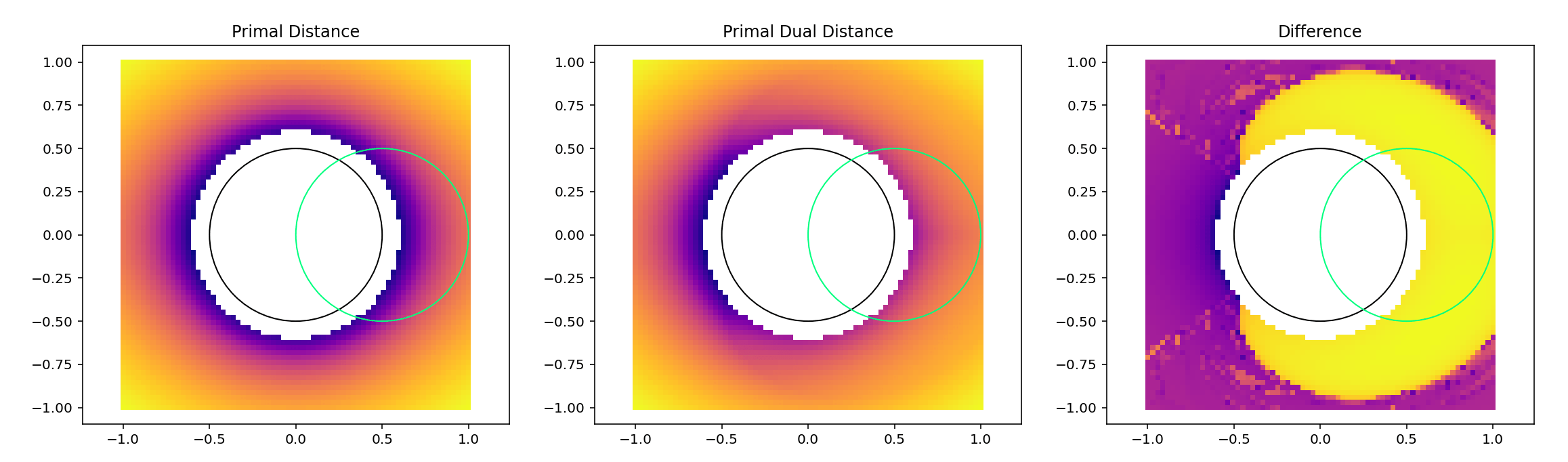
Inverse Dynamics using Motion Set
Primal Only
Primal-Dual
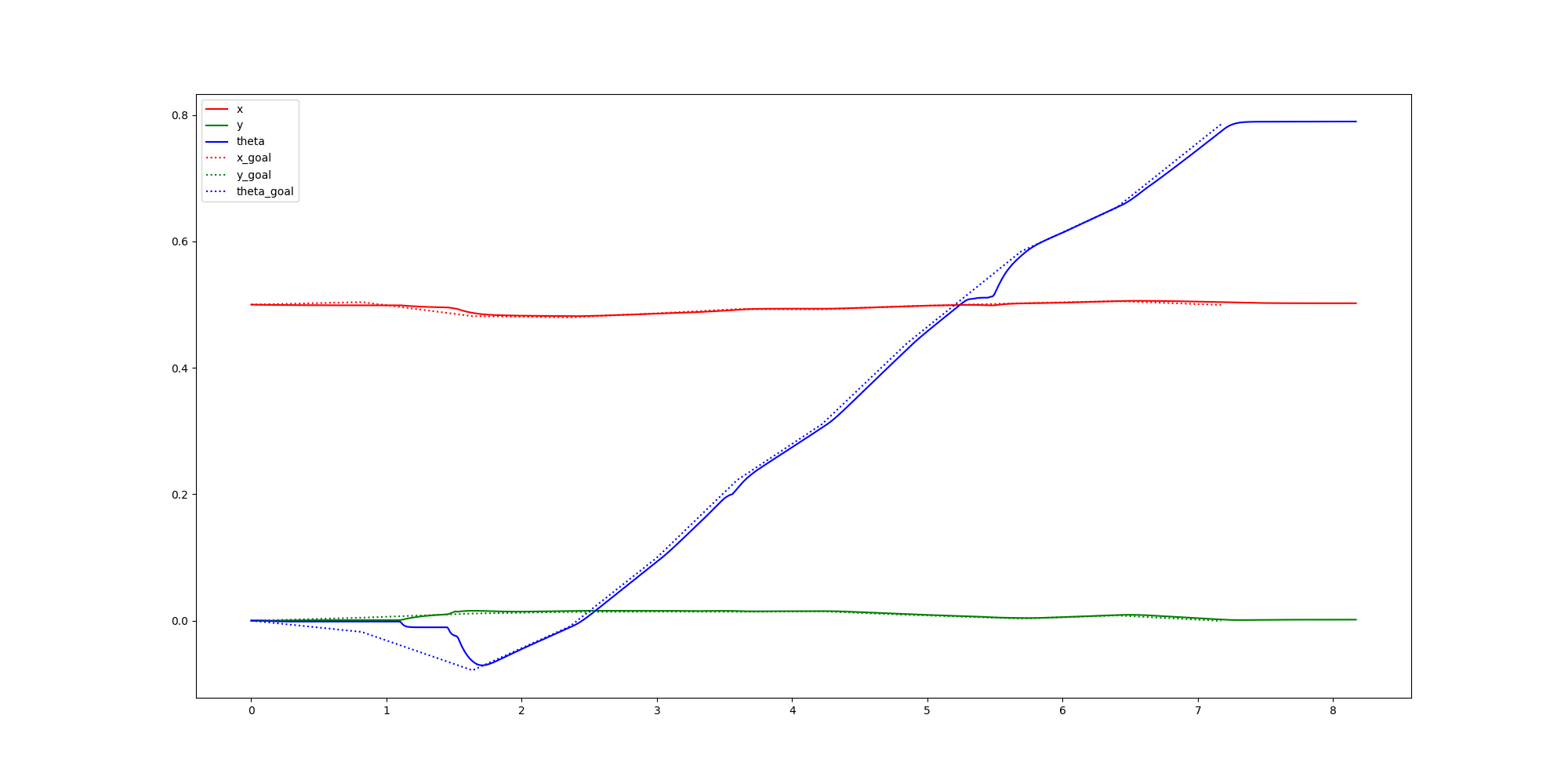
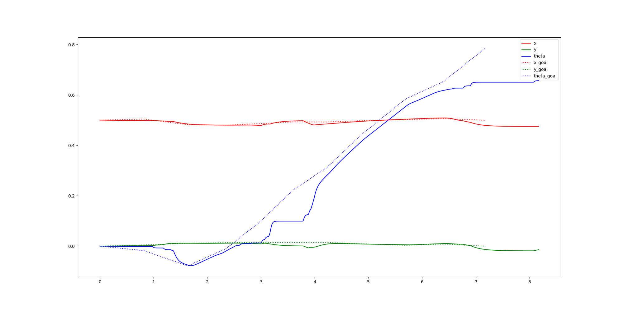
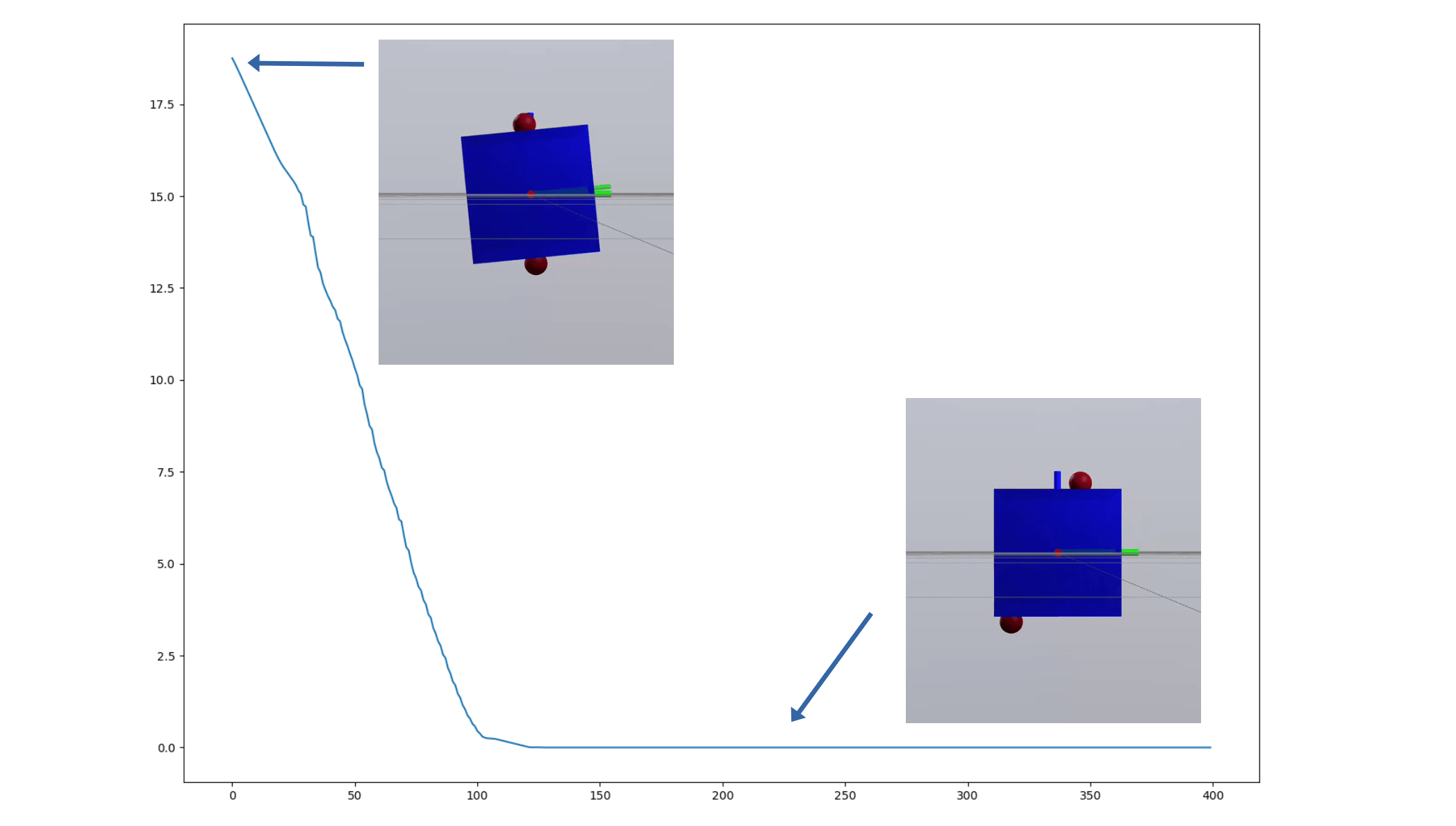
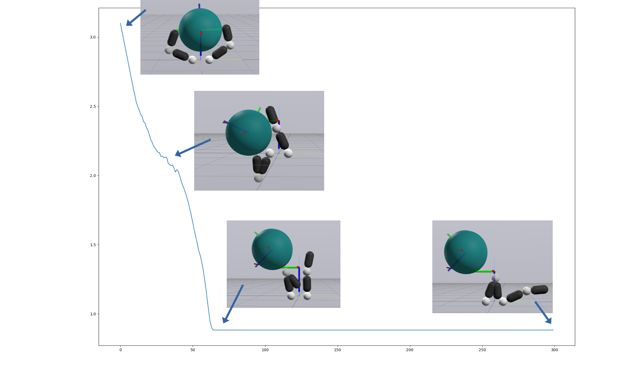
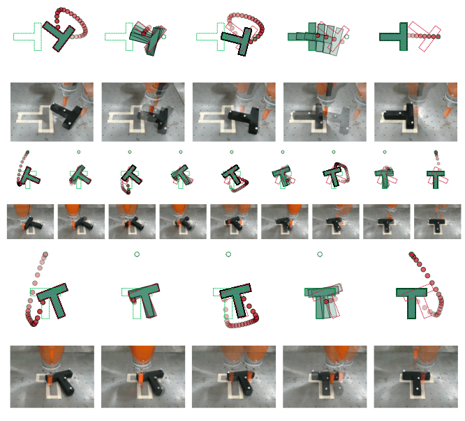
Inverse Dynamics Performance
Primal Only
Primal Dual
First feedback controller (besides MPC) that shows good performance for me
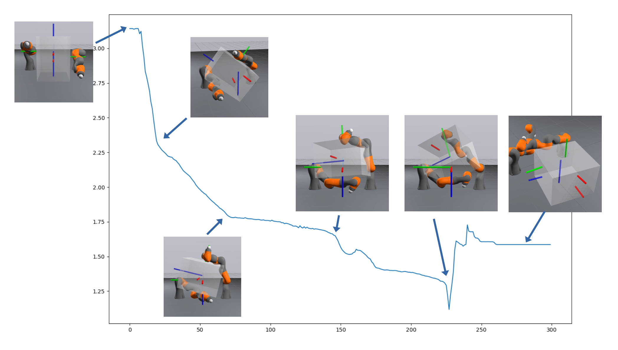
Sim2Drake Performance
Primal Only
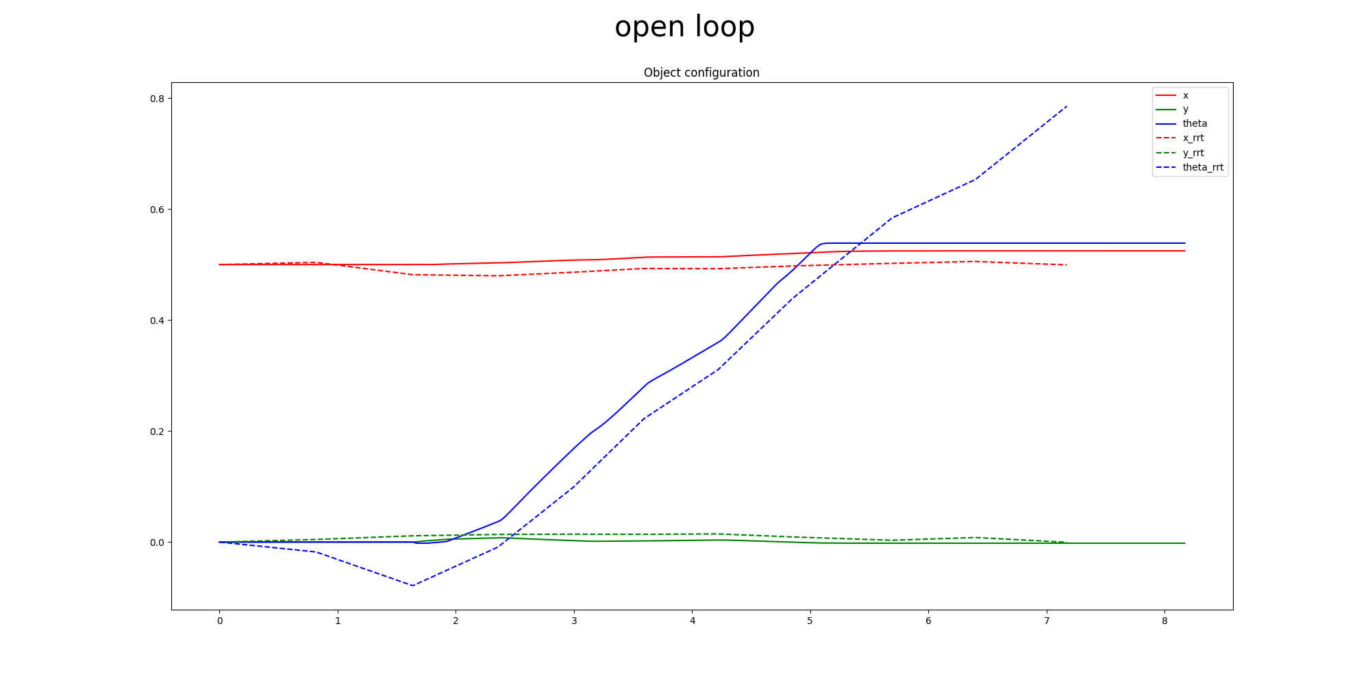
Open Loop
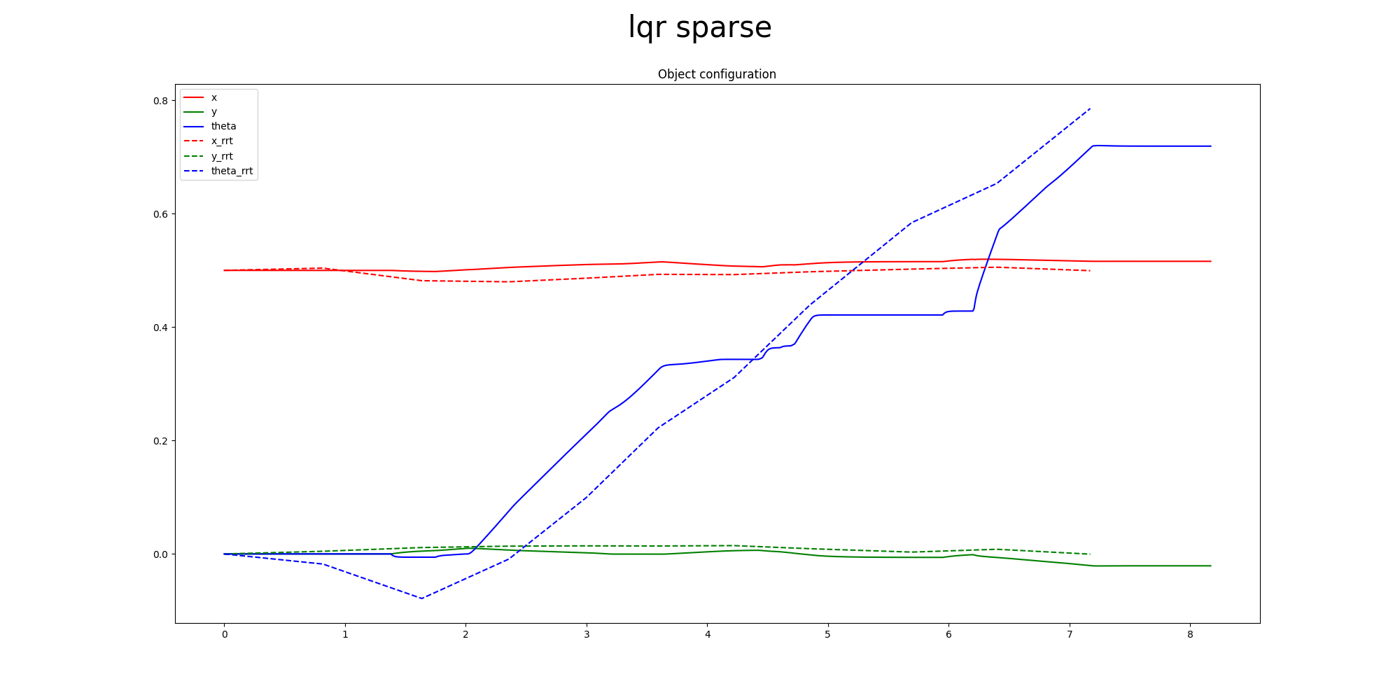
LQR
Primal-Dual
Done by Tong at BDAI
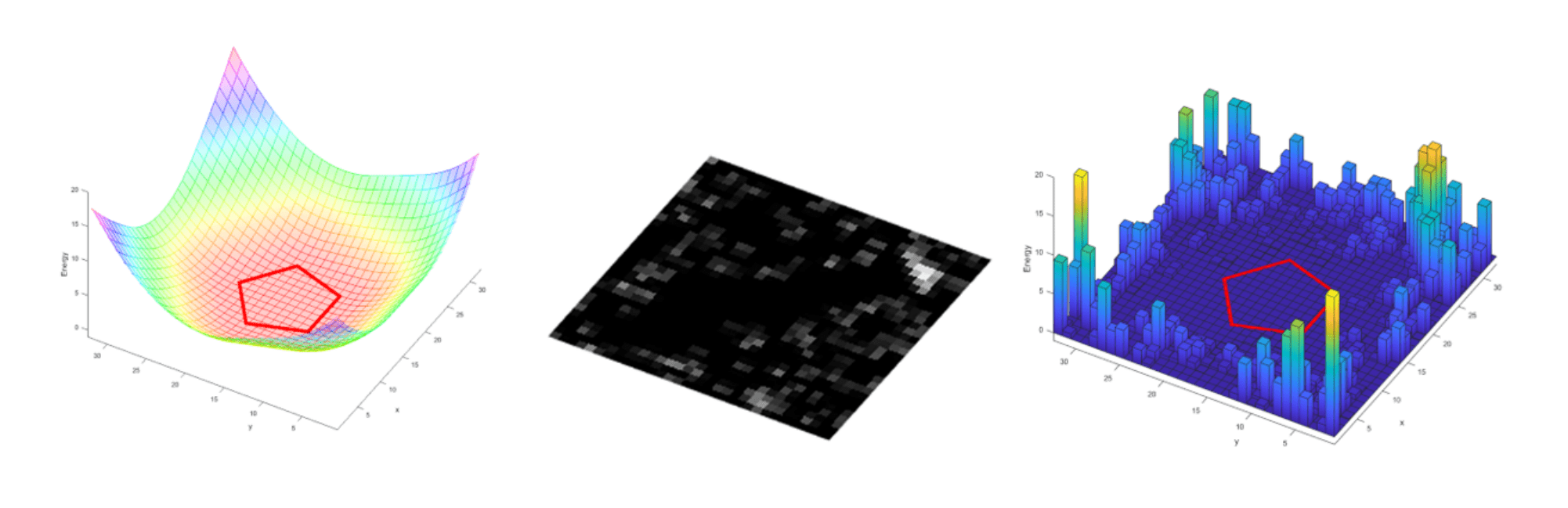
Inverse Dynamics Cost vs. Motion Set
Inverse Dynamics Cost vs. Motion Set
Inverse Dynamics Performance
Inverse Dynamics Performance
Inverse Dynamics Performance
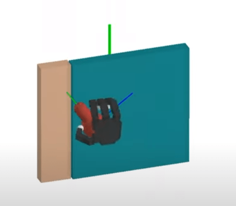
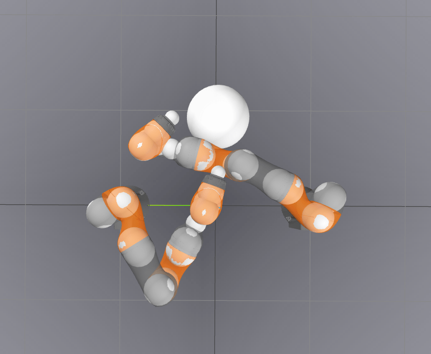
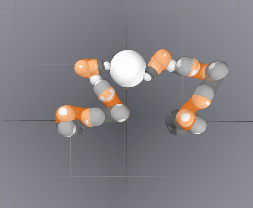
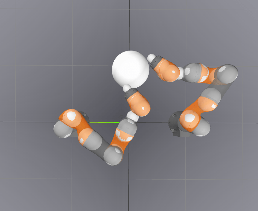
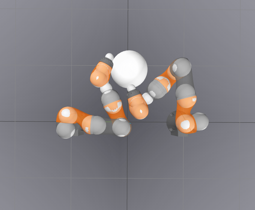
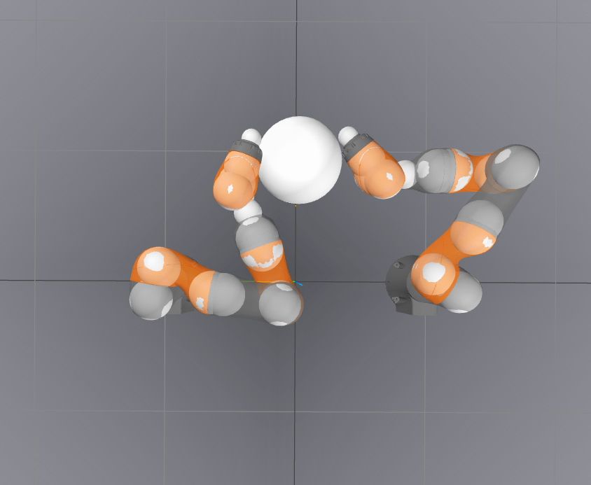
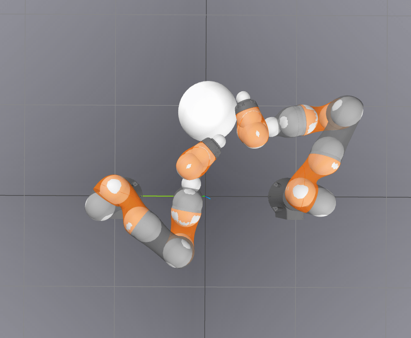
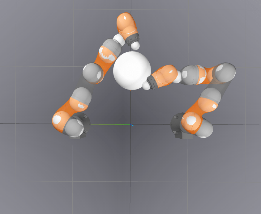
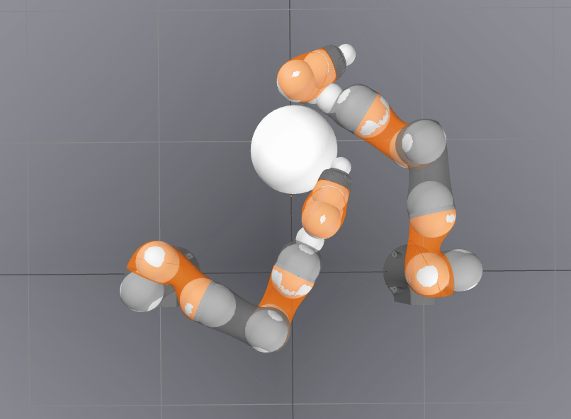
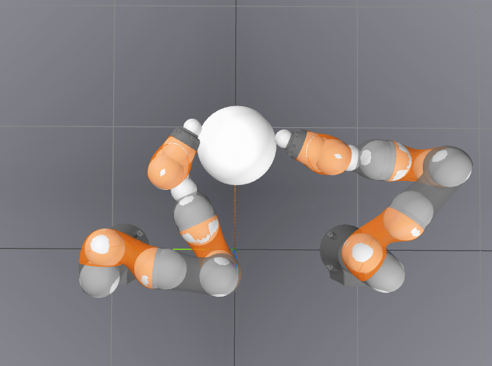
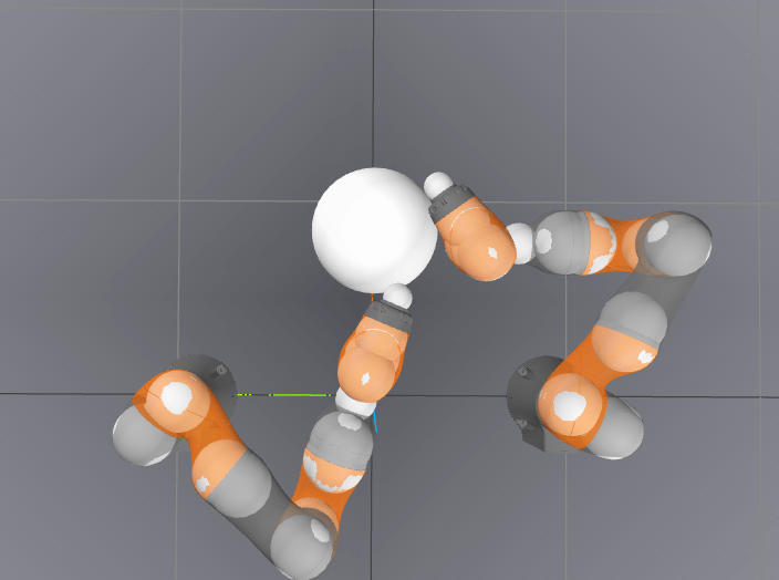
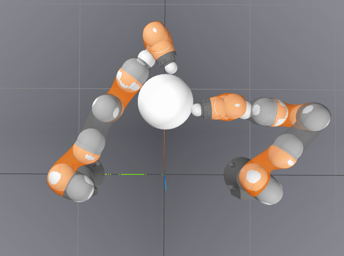
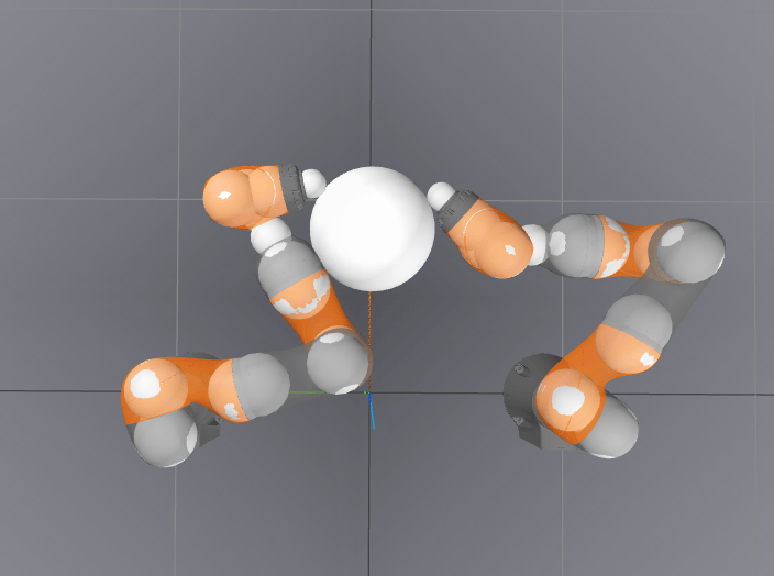
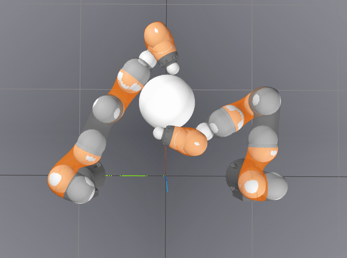
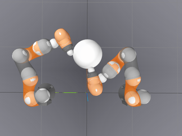
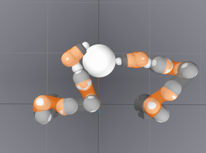
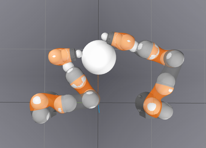
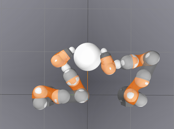
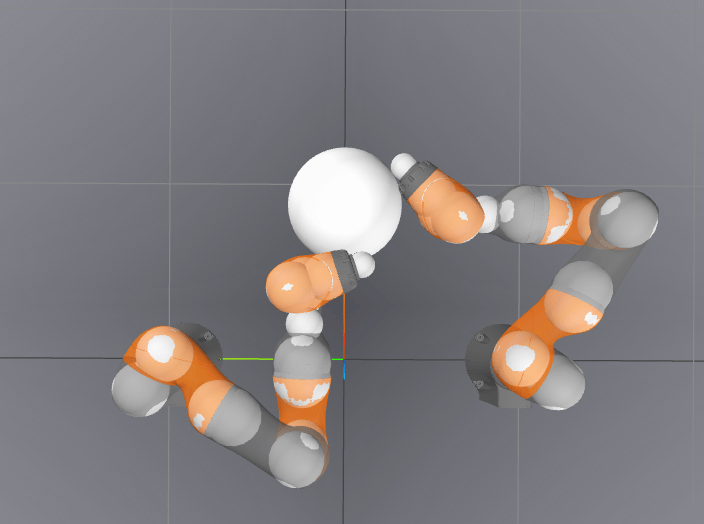
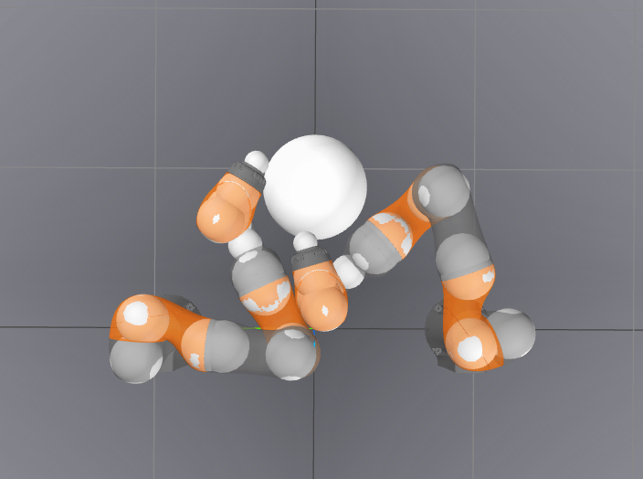
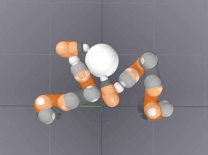
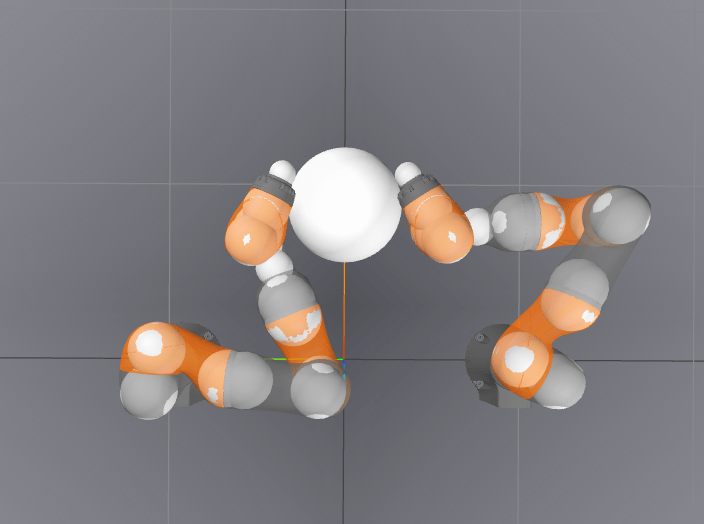
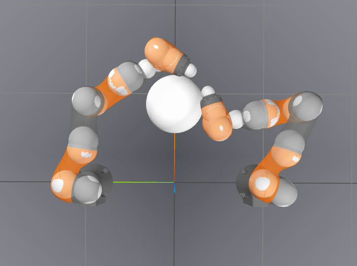
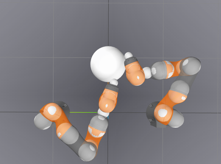
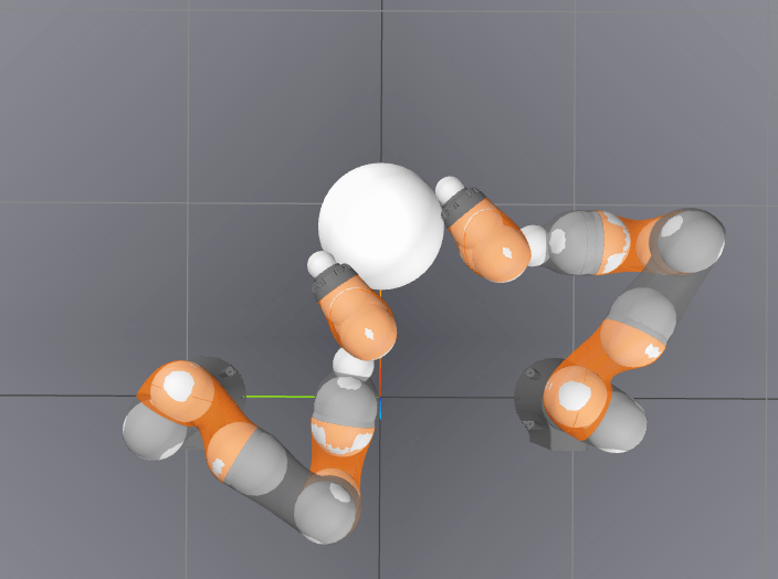
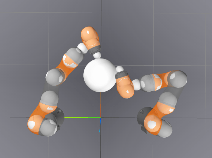
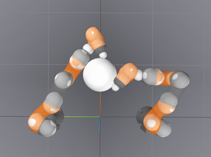
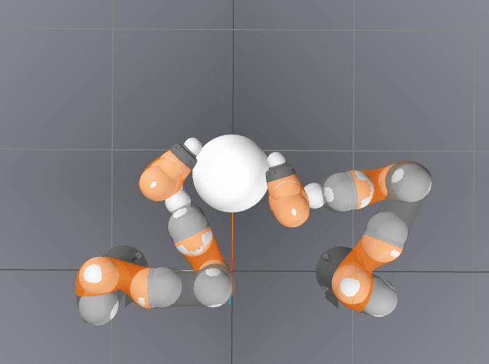
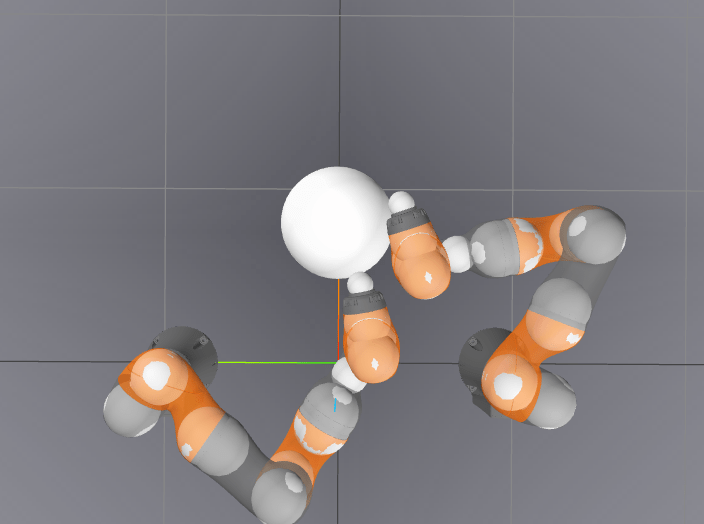
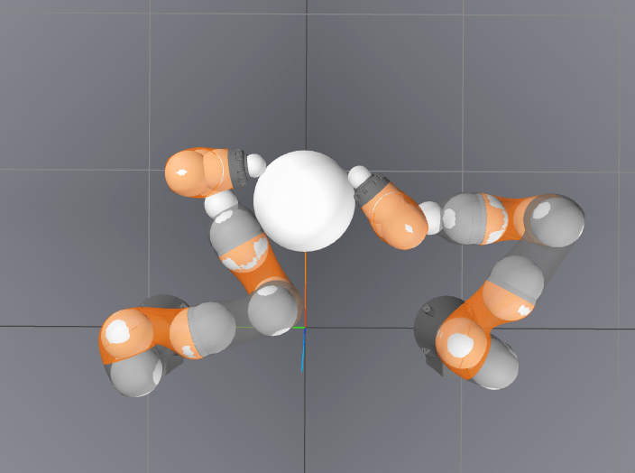
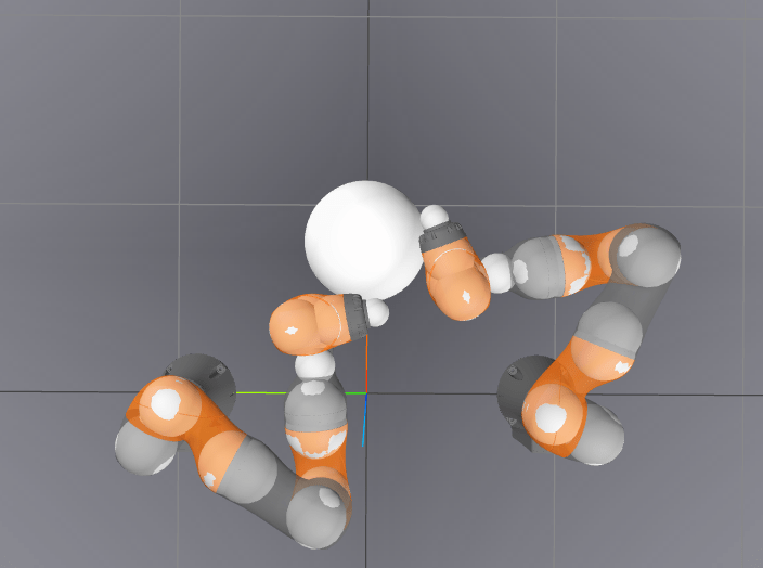
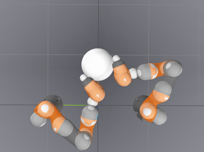
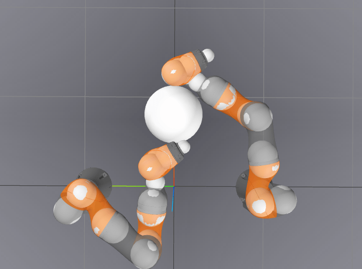
3D In-hand Reorientation
Preliminary Results for Hand
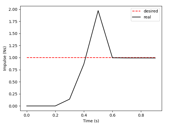
Force Control using Dual Variables
Primal Only
Primal-Dual
Beautifully generalizes to hybrid force/velocity controllers
May allow incorporation of tactile forces when used for estimation
Inverse Dynamics Performance
How far can we go with greedy inverse dynamics?
Why manipulation seems hard

How do we push in this direction?
How do we rotate further in presence of joint limits?

The Action-space problem in Robotics
If we had the wrong action space, the carrot problem hides a horribly difficult planning & control problem.
(Can no longer argue that set distance is CLF)
Motivating the Hybrid Action Space
Local Control
(Inverse Dynamics)
Actuator Placement if feasible
Can running RL / GCS / Online Planning in this action space give us significantly better results?
Same Story
.2s
~80s
The Hybrid Action Space
Local Control
(Inverse Dynamics)
Actuator Placement if feasible
Where do we place the actuators?
What do we mean by feasible?
Where do we do local control to?
How do we choose when to choose between each action?
Quasi-dynamic Feasibility
We're feasible if we're stable.
Distance Metric induced by Reachable Set
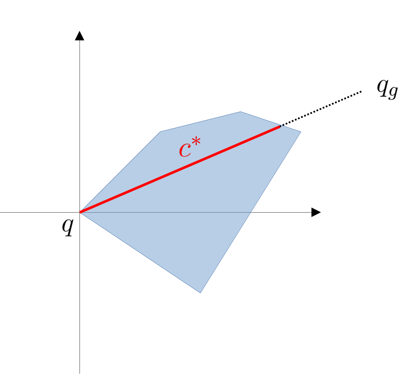
In a finite-input reachable set, the longer we can travel along the ray, the easier it is to reach.
Distance Metric induced by Reachable Set
In a finite-input reachable set, the longer we can travel along the ray, the easier it is to reach.
Distance Metric induced by Reachable Set
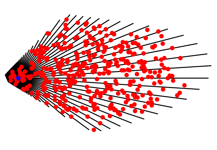
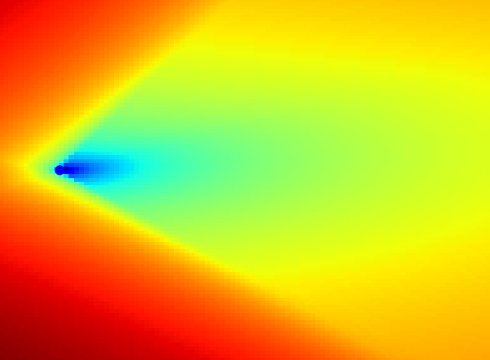
Then, the distance is defined by
regularization
Greedy Solution for Actuator Placement
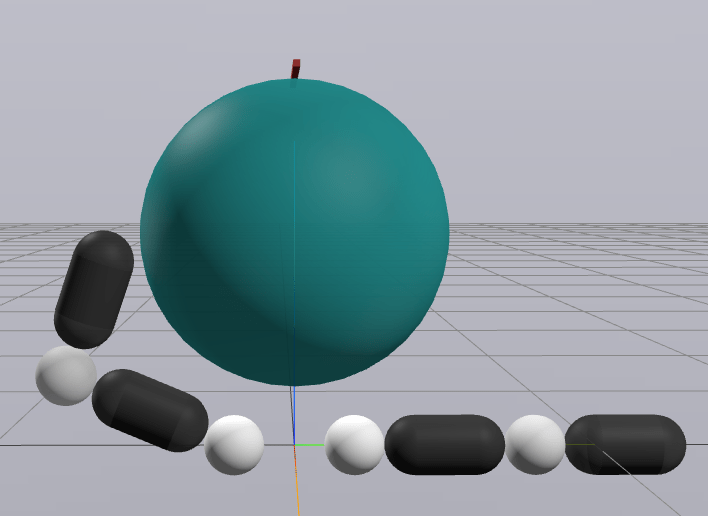
Contact Sampling
The distance metric is incredibly useful for how we should find contacts to begin with.
no penetration
Bad if the goal is towards left.
no penetration
movable actuators
Contact Sampling
Contact Sampling
But doesn't distinguish between these two configurations
If goal is to move right, what's a better configuration?
Contact Sampling
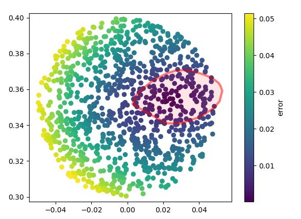
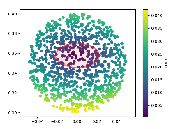
We can add some robustness term from classical grasping
"Maximum inscribed sphere inside motion set".
Contact Sampling
But doesn't distinguish between these two configurations
If goal is to move right, what's a better configuration?
Simple Greedy Strategy
Local Control
(Inverse Dynamics)
Actuator Placement if feasible
Where do we place the actuators?
Where do we do local control to?
How do we choose when to choose between each action?
Find one which will minimize distance to goal according to distance metric.
Always go towards the goal.
Do actuator placement after time T.
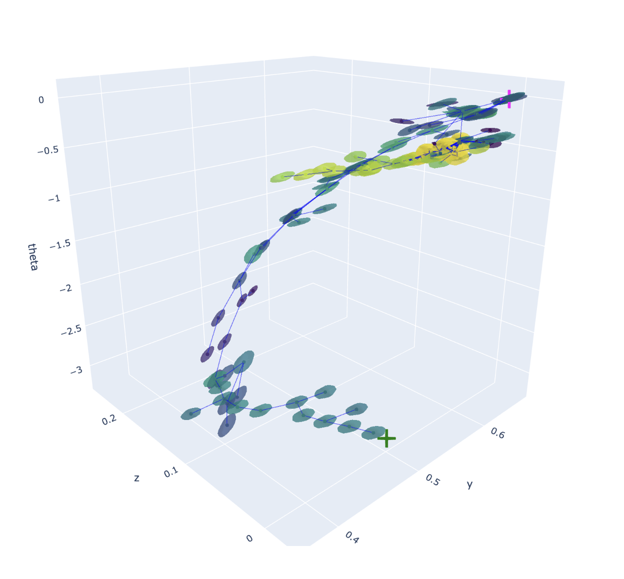
Greedy Planning
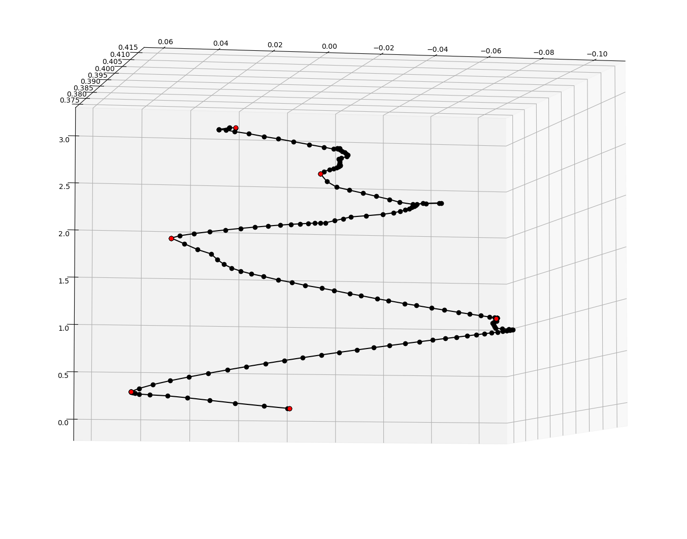
"Sparse graph" induces much less random behavior compared to 1-step based RRT.
Limitations
1
2
3
4
5
6

1
2
3
4
1
2
3
4
The hard manipulation problems are not greedy even in this space!
epsilon-Greedy extension
Local Control
(Inverse Dynamics)
Actuator Placement if feasible
Where do we place the actuators?
Where do we do local control to?
How do we choose when to choose between each action?
Selecting nodes for tree building
Local Control
(Inverse Dynamics)
Actuator Placement if feasible
How do we select which node to grow from?
Results for Tree Search
Tree Search
Greedy
Results for Tree Search
Why not do RRT?
1
2
3
4
1
2
3
4
Where do we do local control to?
Why is sampling from a random direction in a motion set a better strategy compared to choosing subgoals at random?
Asking local control to do reach a subgoal here is very inefficient.
Why not do RRT?
1
2
3
4
1
2
3
4
Asking to go to locally feasible directions is more efficient.
-25.2334 / 0.0000
-2.5983 / 0.0023
-3.9133 / 0.0003
-11.6394 / 0.0002
-1.8232 / 0.0023
-3.6396 / 0.0001
-3.4371 / 0.0008
-2.4071 / 0.0011
-2.1063 / 0.0014
-12.7220 / 0.0001
-4.5312 / 0.0006
-2.7226 / 0.0011
-5.8354 / 0.0020
-10.0993 / 0.0001
-1.6193 / 0.0020
-4.9144 / 0.0007
-4.4108 / 0.0017
-4.3626 / 0.0010
-23.6115 / 0.0001
-3.1907 / 0.0022
-3.8313 / 0.0004
-5.4226 / 0.0005
-7.1475 / 0.0006
-2.7731 / 0.0024
-10.6818 / 0.002
-2.132 / 0.0007
-2.852 / 0.0020
-1.3987 / 0.0017
-7.1905 / 0.0001
-2.8716 / 0.0013
-2.0403 / 0.0012
-1.7866 / 0.0018
Min-weight Metric
Planning
Better Distance Metric w. Motion Sets

Better Extension w. Inverse Dynamics
Better Goal-Conditioned Regrasping
How much does this improve previous planning?
Planning
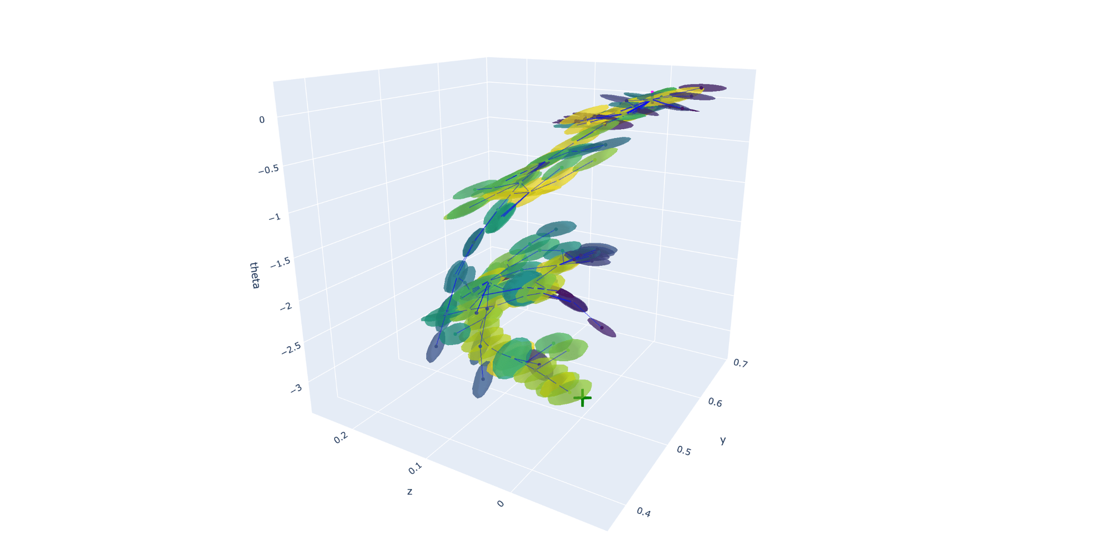
Example old tree
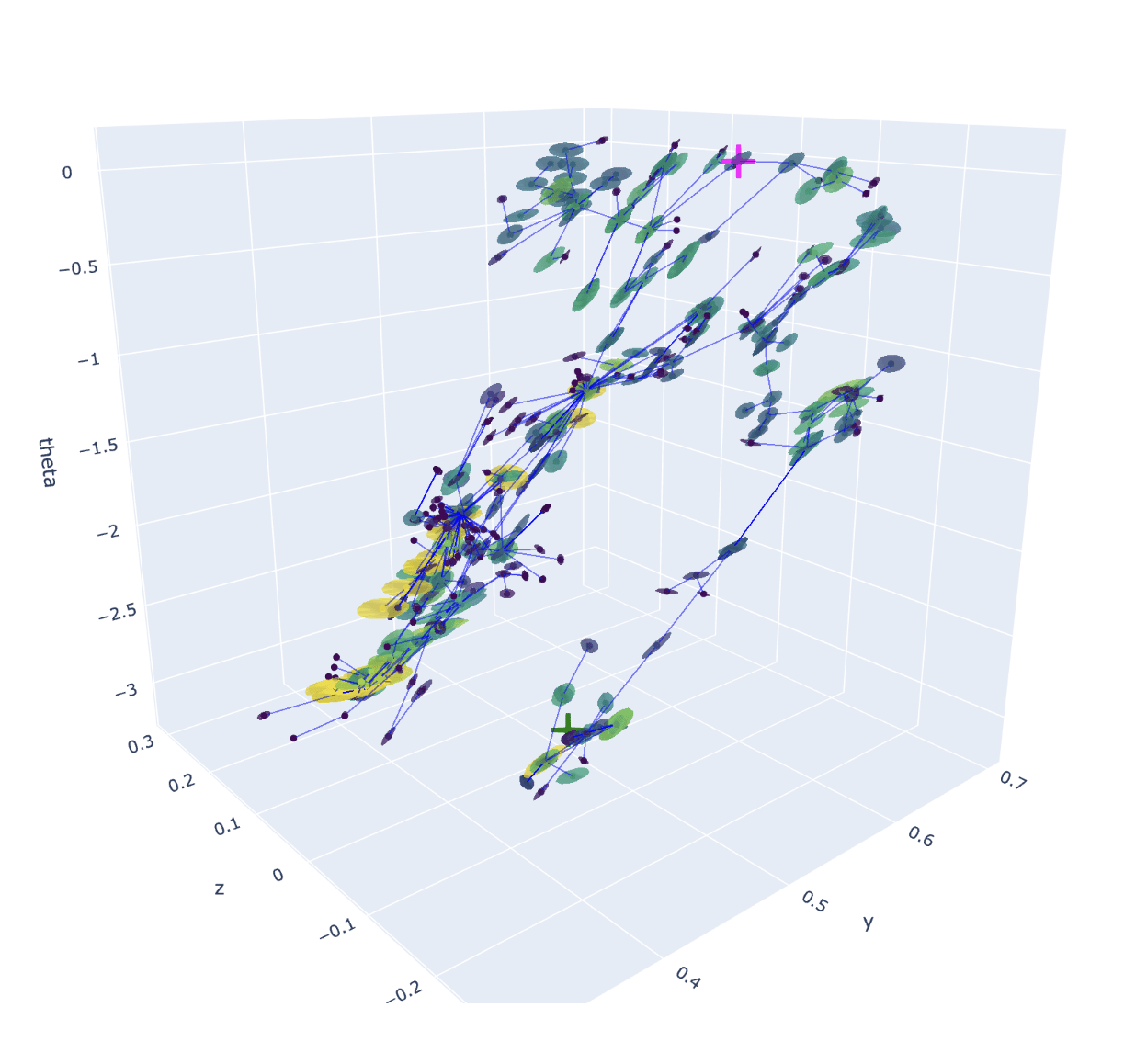
Example new tree
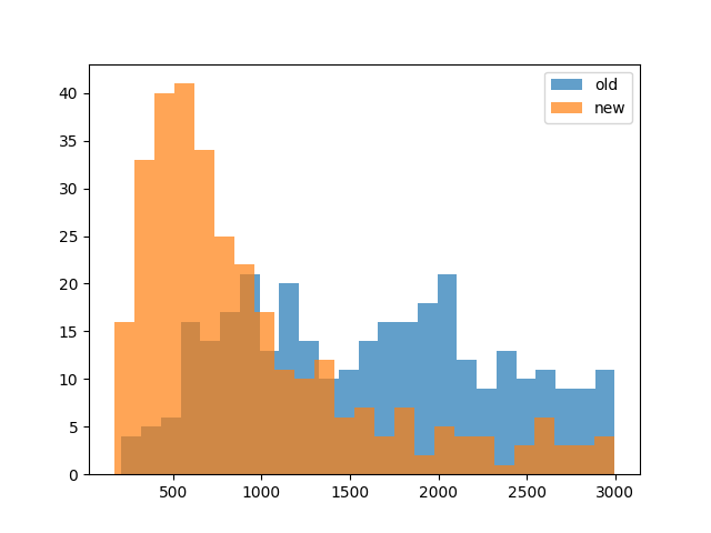
Number of nodes in trees for 320 successful RRTs from random initial object poses
Planning
Current node q
Next node q
Inverse dynamics
Collision-free motion planning
When do we choose between options?