Randomized Smoothing of Optimal Control Problems
RLG Group Meeting 2021 Fall
Terry
Motivation.
- Understand benefits of considering stochasticity in optimal control problems.
- Rewrite RL methods in a more "natural" language for our problems.
- Better computation of gradients of stochastic objectives,
Objectives:
Previous Work:
- Focus on smoothing out the dynamics of the problem.
- Intuitive understanding of what it means to average out dynamics.
- Very practical algorithm for doing planning-through-contact.
- Dynamics proved to be mostly continuous due to infinitesimal time / inelastic impacts.
- Was not able to analyze behavior of smoothing when it comes to discontinuities.
- Not able to analyze the resulting landscape of the long-horizon optimal control problem.
Good points:
Leaves much to be desired...
We want to understand the landscape of value functions. When we lift the continuity provided by time and reason about long-horizon effects, discontinuities and multi-modalities rear their ugly heads.
Problems of Interest Today:
Motivation.


Tomas's pendulum moves between 0 and 1st order gradients.
Differentiable RL? Analytical Policy Gradient? Why? Why not?
Analytical Policy Gradient.
Given the access to the following gradients:
One can use the chain rule to obtain the analytic gradients, that can be computed efficiently using autodiff on the rollout:
Conceivably, this can be used to update the parameters of the policy.
Policy Gradient Sampling Algorithm
Initialize some parameter estimate
While desired convergence:
Sample some initial states
Compute the analytical gradient of the value function from each sampled state.
Average the sampled gradients to obtain the gradient of the expected performance:
Update the parameters using gradient descent / Gauss-Newton.
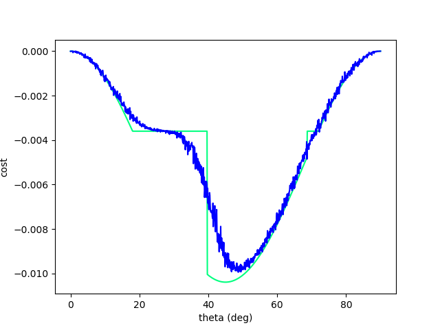
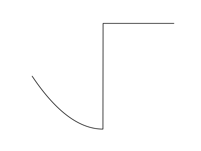
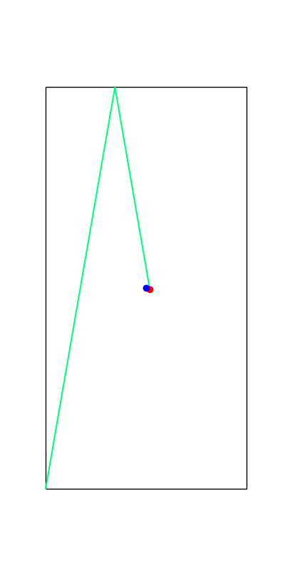
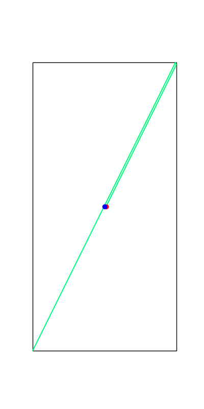
Back to high-school physics: suppose we throw a ball (Ballistic motion) and want to maximize the distance thrown using gradient descent.
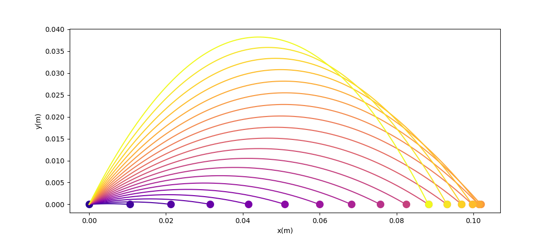
Quiz: what is the optimal angle for maximizing the distance thrown?
Escaping Flat Regions.
Back to high-school physics: suppose we throw a ball (Ballistic motion) and want to maximize the distance thrown using gradient descent.
Quiz: what is the optimal angle for maximizing the distance thrown?
45 degrees!
If we plot the objective as a function of the angle, it is a nice gradient dominant function that will converge to the local minima.
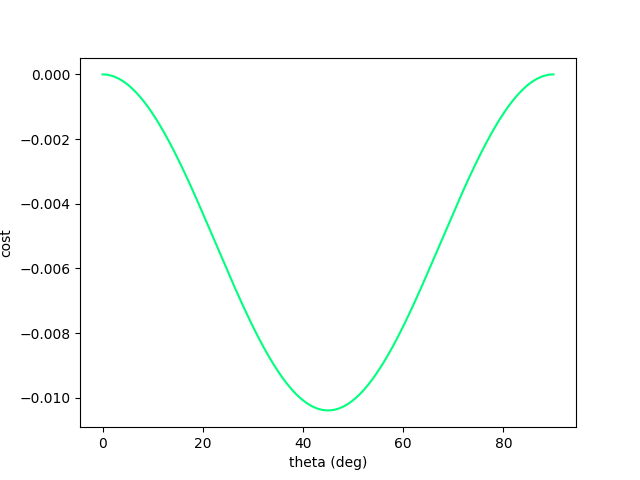
(Interestingly, this is non-convex. Typical example of one of Jack's PL inequality functions).
Escaping Flat Regions.
Back to high-school physics: suppose we throw a ball (Ballistic motion) and want to maximize the distance thrown using gradient descent.
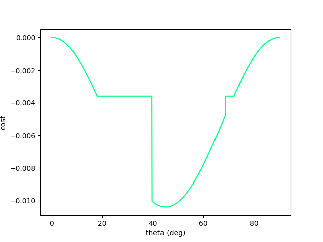
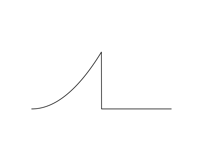
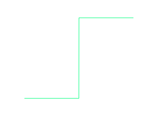
Now we no longer have such nice structure....gradient descent fails.
There is fundamentally no local information to improve once we've hit the wall!
Even though the physical gradients are very well defined, we can no longer numerically obtain the minimum of the function.
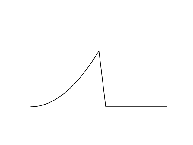
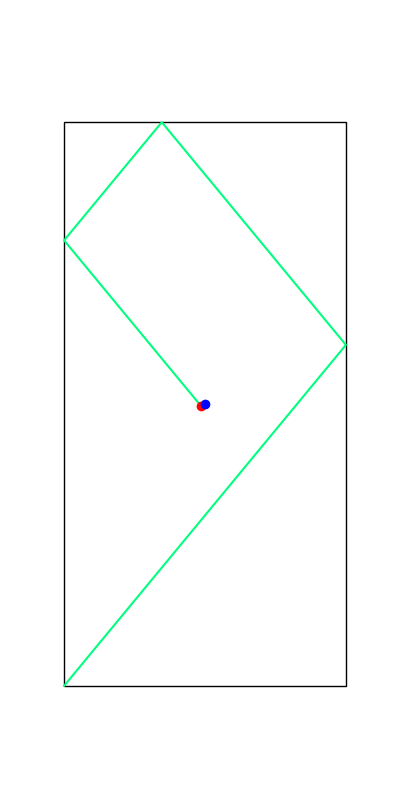
Now let's add a wall to make things more interesting. (Assume inelastic collision with the wall - once it hits, falls straight down)

Escaping Flat Regions.
Back to high-school physics: suppose we throw a ball (Ballistic motion) and want to maximize the distance thrown using gradient descent.
Now we have recover gradient dominance! Now we know where to go when we've hit the wall.
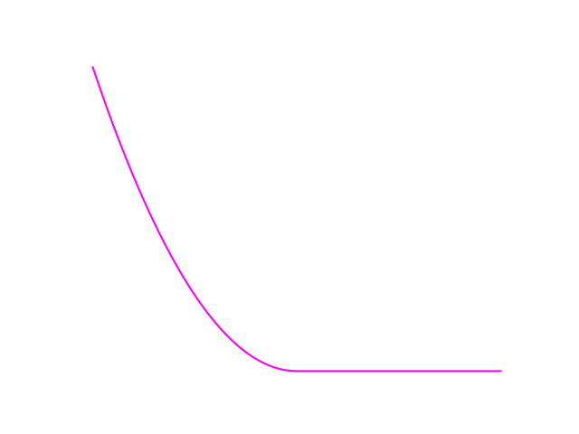
To resolve this, consider a stochastic objective by adding noise to the decision variable:
Escaping Flat Regions.
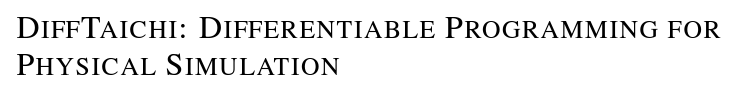
Excerpt from Difftaichi, one of the big diff. sims.
Rather surprising that we can tackle this problem with a randomized solution, without:
- manual tuning of initial guesses
- tree / graph search.
(Or rather, it was surprising to me at the beginning that gradients can't tackle this problem, the problem seems pretty easy and a search direction seems to exist.)
Escaping Flat Regions.
Gradient-Driven Deaths
- Given the objective function , you follow the gradient to maximize the objective.
- The next gradient ascent step points you towards a bad value.
- You fall off a cliff and are unable to recover to where you were before.
Defining Gradient-Driven Deaths
- Not necessarily caused by discontinuity. Also fails on stiff functions with large step size.
- Discontinuities are special in the sense that there is a point at which GDDs happen for all step sizes.
- Once GDD occurs, it can be impossible to recover.
- GDD is insensitive to initial conditions. Wherever you seed, it will occur.
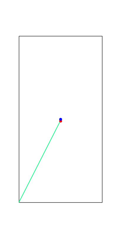
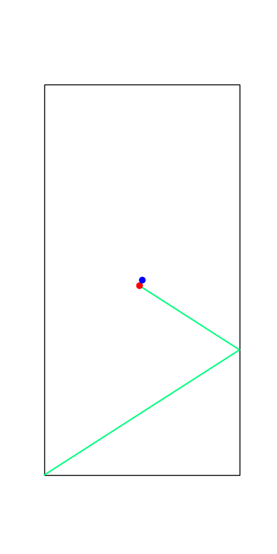
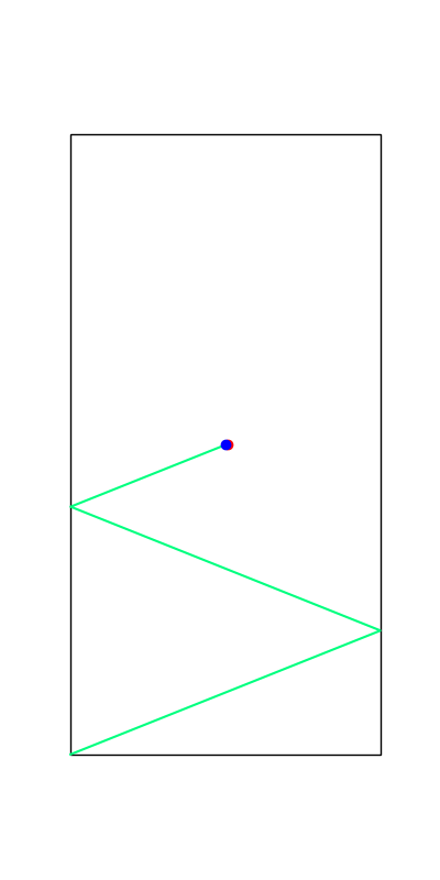
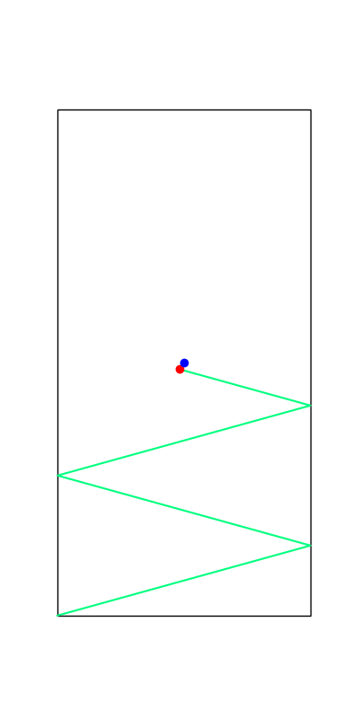
Example 1. Momentum Transfer
1. You need to choose an angle to shoot the hinged door.
2. You get paid based on how much angular momentum you transfer to the door.
3. But if you miss, the hinged door will obviously not move.
Naively following gradients towards optimality makes you fall off the cliff.
(Said another way, there is tension between being optimal and being "safe")
Example 1. Shooting at hinged door.
Example 1. Momentum Transfer
Not a contrived example....
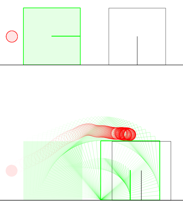
This example quickly figures out that it should maximize moment arm of the pusher, only to end up in a no contact scenario.
Example 2. Manipulation at Dynamic Limits
1. You need to move a cart from point A to point B.
2. You get paid to be as fast as possible, as well as precise (up until here, standard minimum-time DI)
3. But if you drop the ball, you get no points!
Example 2. Minimum-time Transport

Ever got too greedy and failed this task? (Waiter serving drinks?)
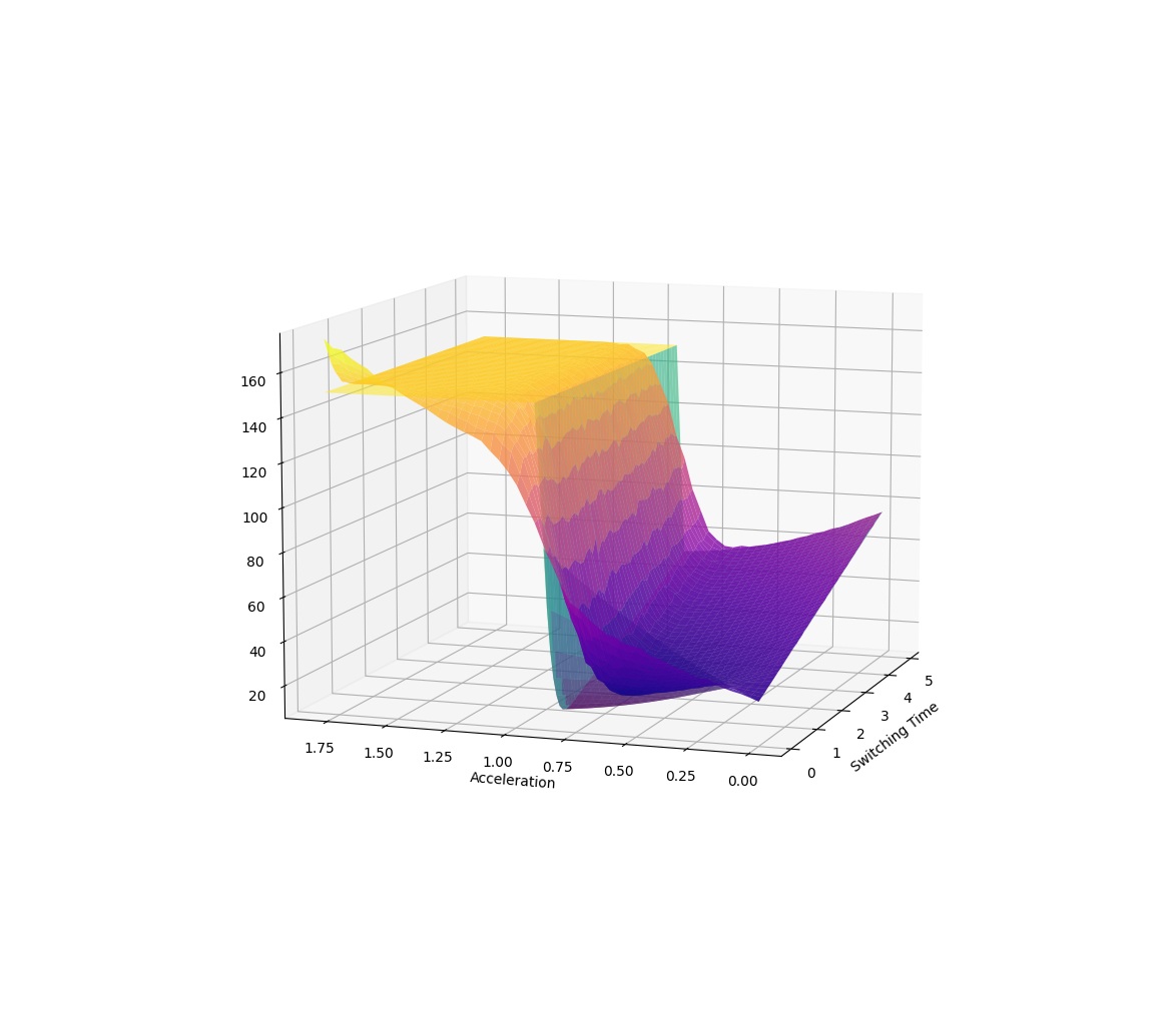
Example 2. Manipulation at Dynamic Limits
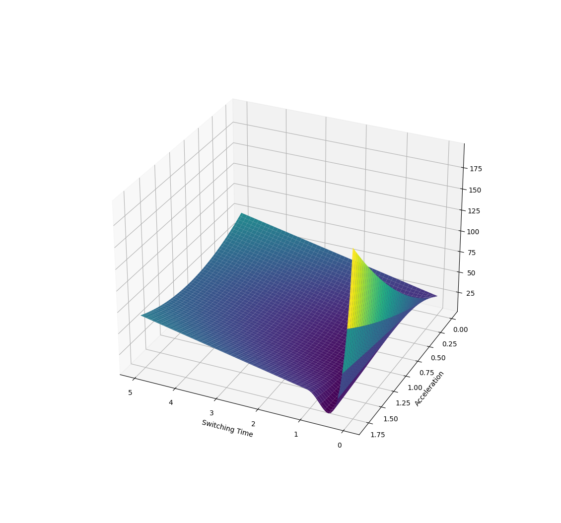
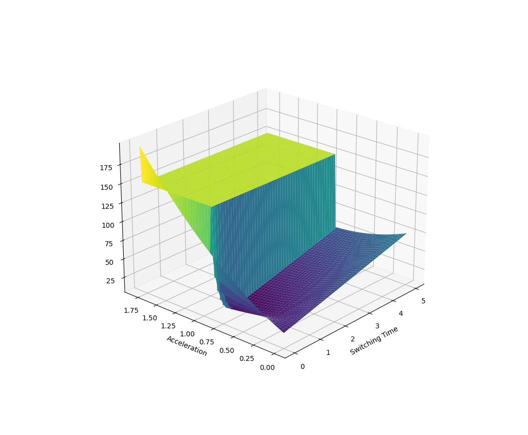
Here the parametrized policy is bang-bang (with two parameters of bang acceleration and switching time)
Example 3. Block Stacking
1. Your job is to find horizontal magnitudes of how much to place the box.
2. You get paid based on how far to the right you stack the box and the height of the stack.
3. But if you become too greedy, the stack might topple!
Example 3. Block stacking
GDDs Recap.
- Optimization problem has tension between optimality and "safety".
- Optimization problem is discontinuous / changes too quickly (high Lipschitz constant).
- Gradient only reasons about local behavior (limit as epsilon goes to zero)
Why do GDDs occur?
How should we prevent GDDs?
- Add and use constraints! (climb as high as possible s.t. I don't fall off a cliff)
- RL doesn't have constraints....why doesn't RL as optimization have this problem?
Sometimes, constraints are difficult to define.
- Stability of boxes might be clear, but what about stones? humanoids?
- Should we constrain the ball to touch the box? Sometimes equivalent to fixing mode sequences.
- Valuable to "implicitly" have constraints from black-box data when the engineer cannot design one with domain knowledge.

Stochastic Objectives
How should we prevent GDDs?
Maybe if we're not so myopic, we'll be able prevent GDDs before they occur.
If we consider a stochastic objective, how would the landscape change?
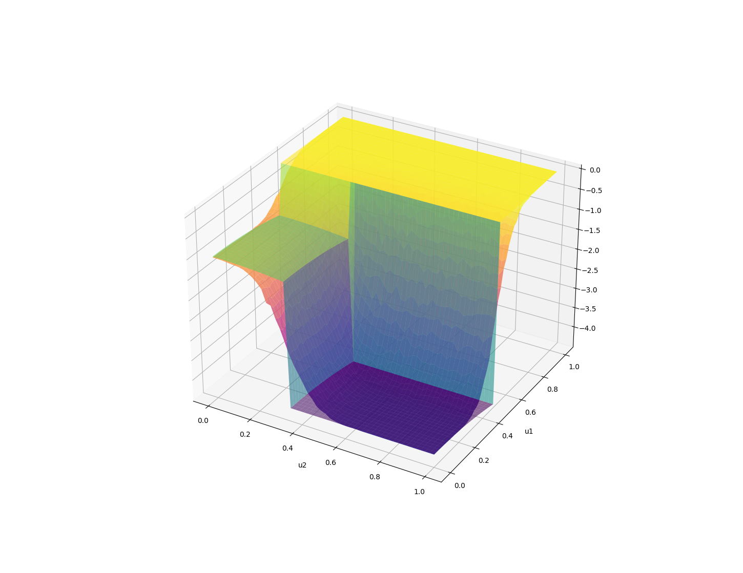
Randomized Smoothing of Value Functions
Original Problem w\ GDDs
Surrogate Stochastic Problem (Bundled Objective)
Example 1. Momentum Transfer
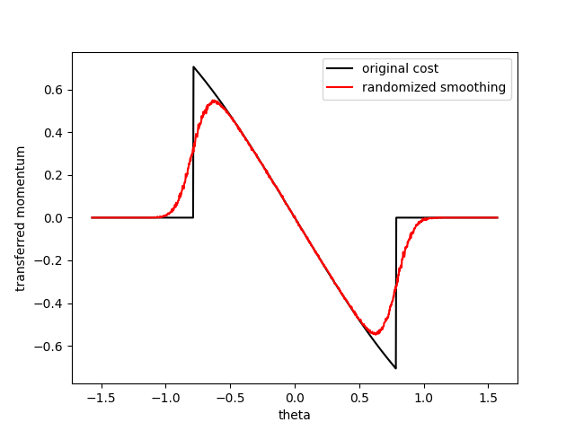
Some samples will hit the door, some samples will miss - the average gives information that we should be more conservative when we do gradient ascent.
Example 1. Shooting at hinged door.
Connection to robust optimization.
Intuitively satisfying answer: the maxima of the bundled objective is "pushed back" by how uncertain we are.
Example 2. Manipulation at Dynamic Limits
Some samples will drop the payload, some samples will not. Behaves better on average.
Connection to robust optimization.
Intuitively satisfying answer: the maxima of the bundled objective is "pushed back" by how uncertain we are.
Example 2. Minimum-time Transport
Example 3. Block Stacking
Similarly, the expected value behaves much better.
Example 3. Block stacking
GDDs can be eliminated by considering a stochastic formulation of the objective!
Emergence of Constraints from Stochasticity
Mathematical Characterization of this behavior:
If the function has a high-cost region, we can decompose the function into:
Expectation is a linear operator, so we can smooth them out individually and add them back in.
By taking an expected value, we have something that resembles more the Lagrangian of the optimization
if we had explicitly wrote down the constraint.
Emergence of Constraints from Stochasticity
Connection to Interior-Point Methods
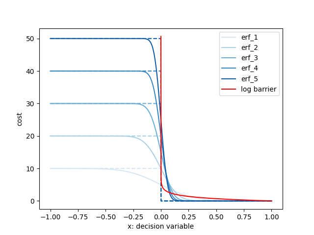
Consider the canonical log-barrier function:
Smoothing creates a barrier function-like effect that encourages adherence to constraints.
Emergence of Constraints from Stochasticity
Madness? More interesting than it seems....
Emergence of Constraints from Stochasticity
Penalizing for collision and sampling has the same effect as encoding non-penetration as explicit constraints, then IPOPT taking a barrier-function formulation of it.
(In fact, it might perform better when we start having strange geometries!)
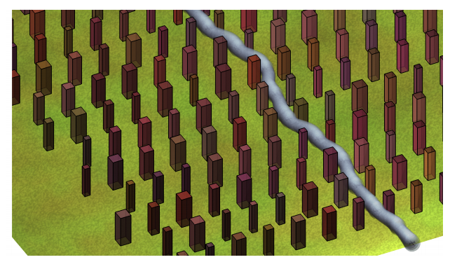
Trajectory Optimization through Forest.
Figure from Ani's paper.
Discussions
Explicit Constraints vs. Soft Constraints from Sampling
- We never needed to actually specify what the constraints should be. This can be a big advantage sometimes.
- The reward / cost simply needs to be able to assign bad costs to bad events (but finite!)
- It is a "soft" constraint - it can be violated (feasibility is not a binary thing).
- But the violation can also work out to your advantage (e.g. can explore mode sequences)
- But such line of thinking may easily lead to games of reward shaping.
Randomized Smoothing on Value Functions
Original Problem
Surrogate Problem
Original Problem (Single-shooting formulation)
Surrogate Problem
expectation over entire trajectory of noises
Injecting noise in policy optimization
Injecting noise in trajectory optimization
Original Problem (Single-shooting formulation)
Surrogate Problem
expectation over entire trajectory of noises
Injecting noise in trajectory optimization
Note: Comparison with Previous Work
expectation over noise in a single timestep.
Randomized Smoothing on Value Functions
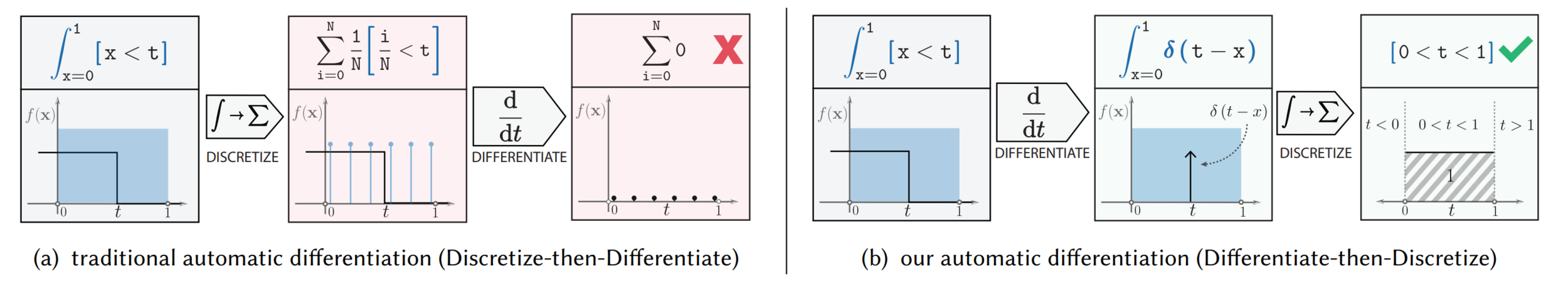
Computing Gradients of Stochastic Objectives
Now let's talk about gradient computations.
Given that has differentiable almost everywhere but has jump discontinuities, how should we compute the gradient of the stochastic objective?
Quantity to compute / estimate:
Recall: The usual trick of D.C.T and Monte-Carlo doesn't work!
Back to our good old example....
Computing Gradients of Stochastic Objectives
We'll review three methods of how to resolve this.
- Use the zero-order numerical gradient.
- Bootstrap the function to a smooth function approximator.
- Analytically add back the Gaussian to the derivative.
Method 1.
If we use finite differences instead of gradients, the interval is not zero-measure, and will always be able to capture the discontinuity.
- Captures the behavior that we want nicely, but very difficult to analyze since we can't use Taylor.
- Usually suffers from higher variance, which leads to worse convergence rates.
Computing Gradients of Stochastic Objectives
Method 2. Bootstrapping to a smooth function approximator.
An effective solution, if you had lots of offline compute, is to simply find a differentiable representation of your discontinuous function by function fitting.
Computing Gradients of Stochastic Objectives
1. Evaluate the bundled objective at finite points:
2. Regress on e.g. neural network to find a surrogate function that is differentiable everywhere:
3. Compute the derivative of the surrogate function.
Doesn't "feel" right to me, but the learning people love this trick!
Bootstrapping to a smooth function approximator.
Computing Gradients of Stochastic Objectives
From DPG paper:
- If the Q function is discontinuous, won't they have the same issue?
- Not if they bootstrap a neural network to approximate Q!
Conv. w/ Abhishek
Likely, many learning methods bypass the problem with discontinuities by spending offline time to store discontinuities into continuous functions.
Of course, comes with some associated disadvantages as well.
Carrots example.
Computing Gradients of Stochastic Objectives
- Q: Why do we need neural simulators?
- A: Because we need gradients.
Conv. with Yunzhu:
Conv. with Russ:
- Q: Why don't you like the word "differentiable physics"?
- A: Physics has always been differentiable. Drake already gives you autodiff gradients through plant.
Resolution?
Perhaps gradients of the smooth representation of the plant can sometimes behave better than true plant gradients.
Very noisy landscape.
Bootstrapped to NN
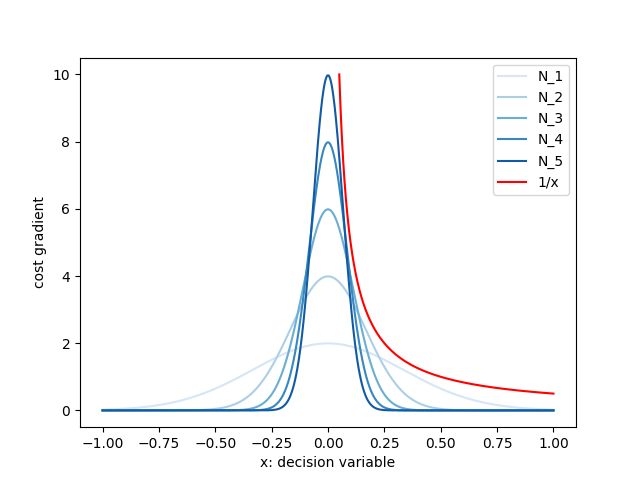
Analytically adding back the Gaussian.
There is actually a quite easy solution to the delta issue if we really wanted to sample gradients....
Computing Gradients of Stochastic Objectives
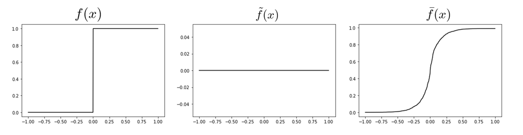
WLOG Let's represent the scalar function having discontinuities at x=0 as:
with
Then we can represent the gradient of the function as:
Gradient sampling fails because we have zero probability of landing at the delta
(and we can't evaluate it if we do anyways....)
Analytically adding back the Gaussian.
So instead of sampling the entire gradient, we can analytically integrate out the delta, then sample the rest.
Computing Gradients of Stochastic Objectives
Taken from "Systematically Differentiating Parametric Discontinuities", SIGGRAPH 2021.
Analytically adding back the Gaussian.
So instead of sampling the entire gradient, we can analytically integrate out the delta, then sample the rest.
Computing Gradients of Stochastic Objectives
Decompose the integral into components without delta (top row), and the delta (bottom row).
Scaling to higher dimensions is challenging.
So how do we scale this to higher dimensions? Starts becoming real complicated....
Computing Gradients of Stochastic Objectives
Derivative of heaviside is the delta, but what is the derivative of a 2D indicator function?
Does such a thing as make sense? Infinity at but ?
Consistent with the 1D delta? Many questions.
Convolution with 2D Gaussian gives a "ridge" of Gaussians,
Computational approach might be to find the closest surface of discontinuity, then evaluate the Gaussian centered at the closest point.
Non-convexity
Smoothing can generally help get rid of high-frequency features in the problem.
- Makes intuitive sense, but hell of a problem to isolate and analyze.
- Can't say much for arbitrary landscapes, even if we confine to smooth functions.
- About to give up on this route....just leave it as a folk legend.
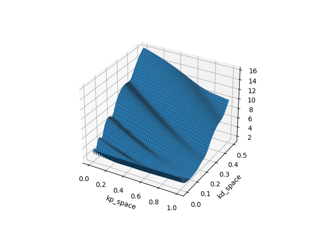
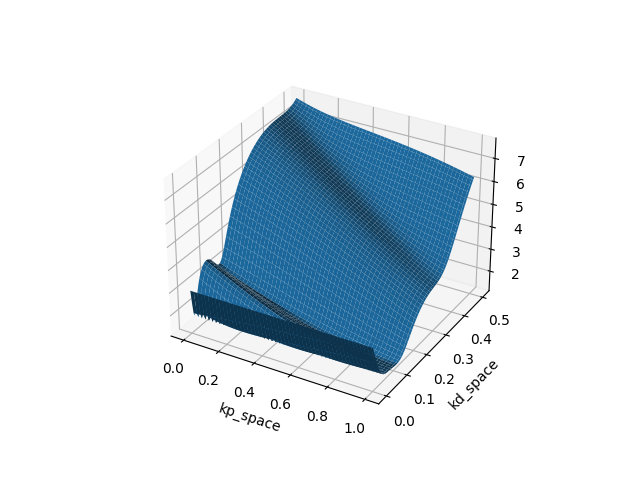
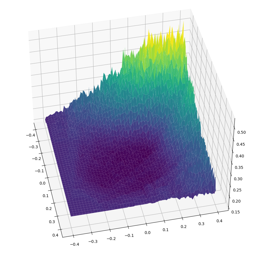
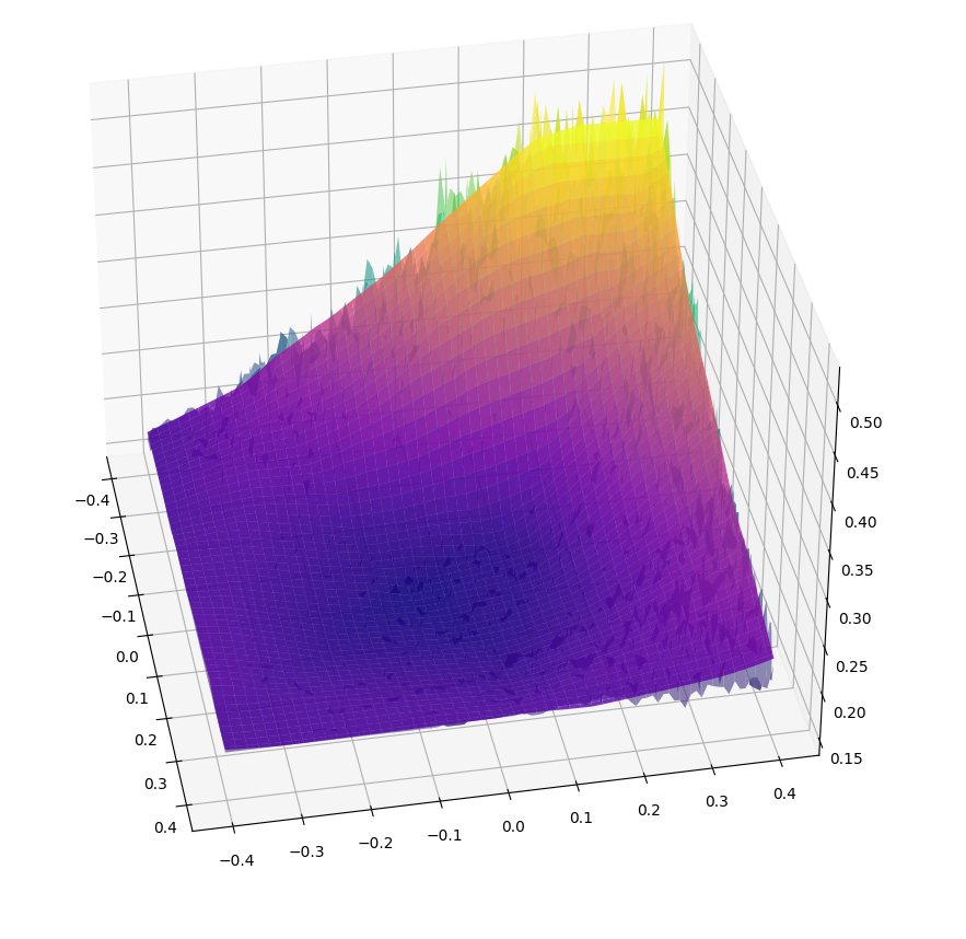
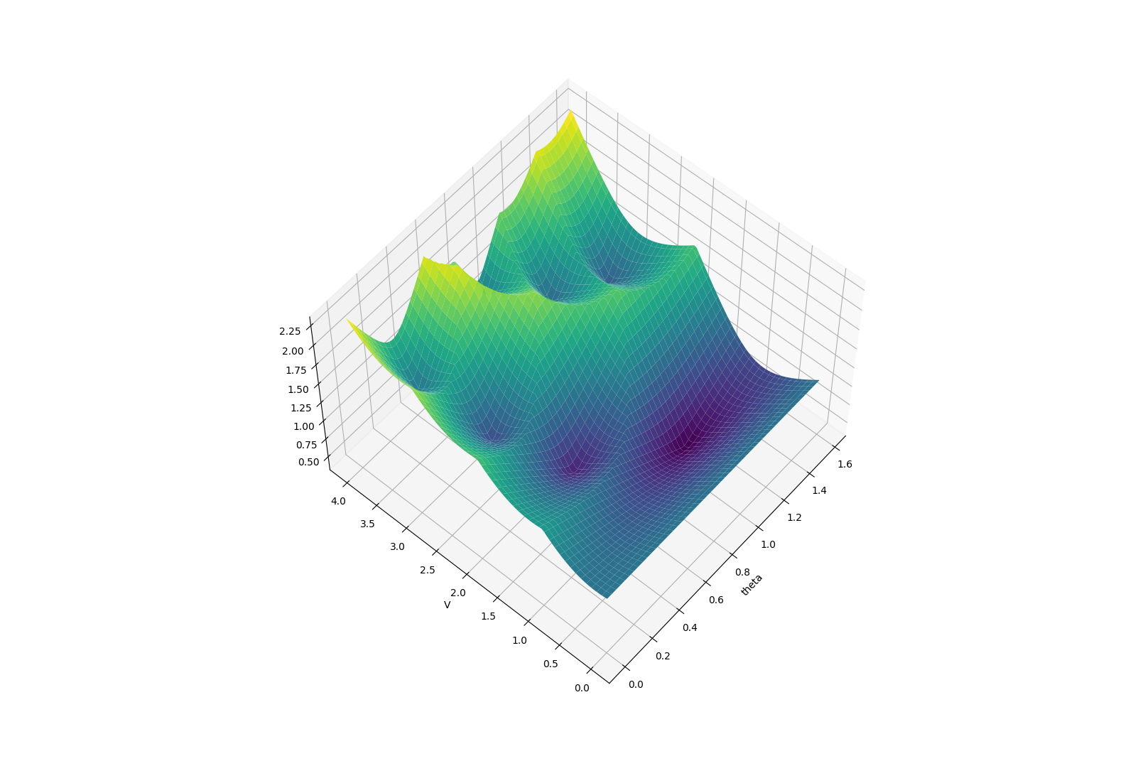
Example: Finite-Horizon LQR on Double Integrator (Policy search on PD gains)
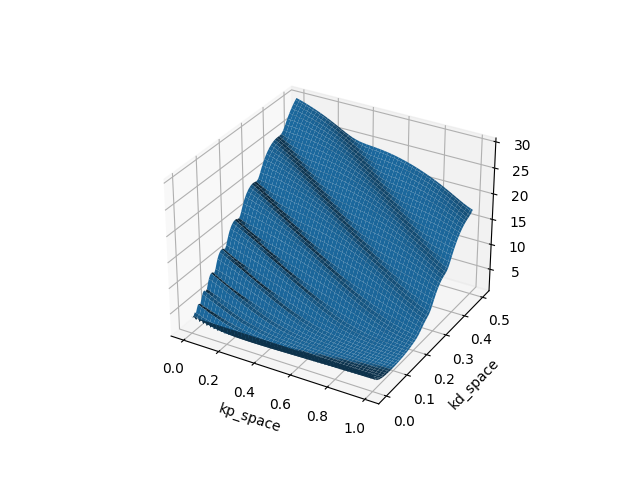

T=10
T=20
T=40
T=80
Which type of "minima" does smoothing prefer? and why?
When Smoothing Hurts
In general, the reasoning about quality (suboptimality) of the different minima is NP-hard.
Instead, we can reason about the behavior of what happens to the boundary points of local minima.
One tool we might be able to use is the region of attraction for different local minima.
Idea is to carve up the domain of the decision variables and "color" them according to different local minima.
How will the boundary of two different regions move as we smooth it out?
Which type of "minima" does smoothing prefer? and why?
Direction of movement of the local maxima is determined by:
Simple 1D example - a local maxima must lie between two local minima, so we reason about what happens to the local maxima as we smooth out the function.
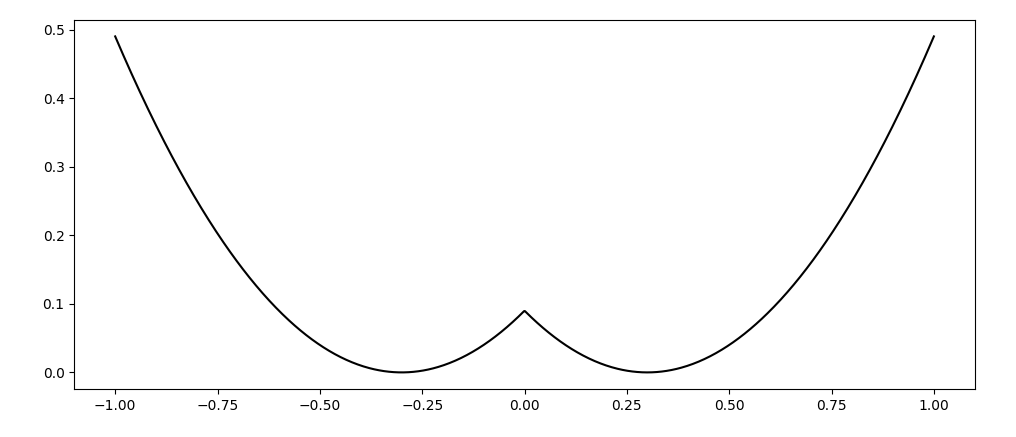
Intuitively, smoothing widens the region of attraction for local minima that have higher Lipschitz constant.
(Prefers to widen "sharp" peaks).
When Smoothing Hurts
When Smoothing Hurts
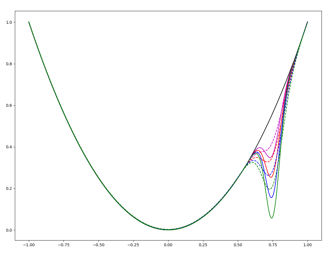
If there is a sharp suboptimal local minima, the region of attraction of the global minima shrinks.
(But could be the other way around - smoothing helps if there is a sharp global optima with small ROA).
Limitations. Mode Explorations
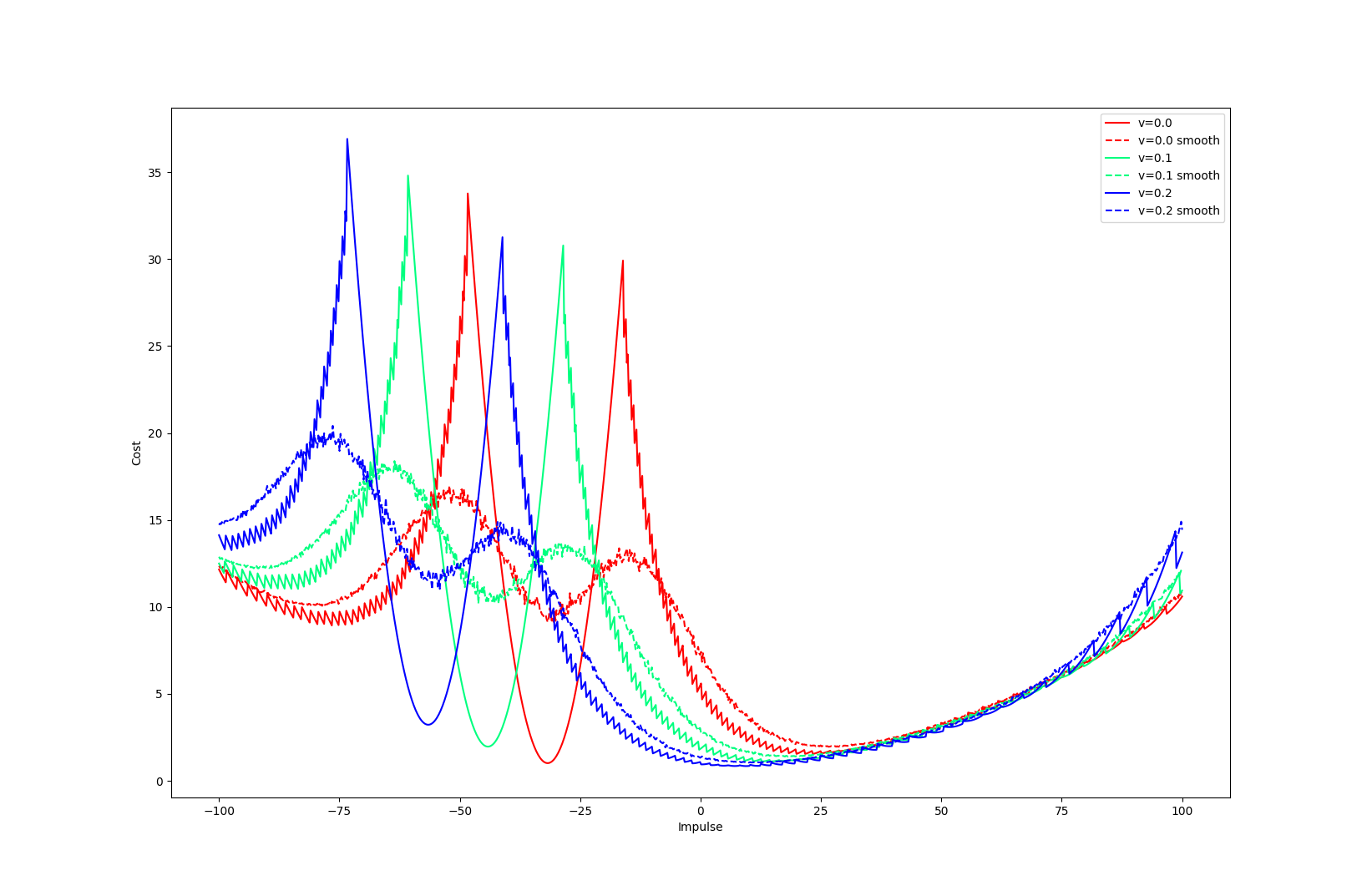
Tobia's example of push recovery
Smoothing doesn't help us find better minima here....
Apply negative impulse
to stand up.
Apply positive impulse to bounce on the wall.
Limitations. Mode Explorations