Group Meeting Spring 2023

Optimal Control and Policy Search

\begin{aligned} \min_\theta\quad & \mathbb{E}_\rho\left[c_T(x_T) + \sum^{T-1}_{t=0} c(x_t,u_t)\right] \\ \text{s.t.}\quad & x_{t+1} = f(x_t, u_t) \quad \forall t \\ & u_t = \pi_\theta(x_t, t) \quad \forall t \\ & x_0 \sim \rho(x) \end{aligned}

In its most general statement: Find parameters of my policy to optimize some cost.

- Note this formalism is super broad. Trajectory optimization, dynamic policies, all included.

Typical discrete-time finite horizon optimal control (policy search)

Optimal Control with Distribution Risk

Given some reference distribution p(x,u), penalize how much we deviate away from the distribution.

\begin{aligned} \min_\theta\quad & \mathbb{E}_\rho\left[c_T(x_T) + \sum^{T-1}_{t=0} c(x_t,u_t) - {\color{blue} \beta\sum^{T-1}_{t=0} \log p(x_t,u_t)}\right] \\ \text{s.t.}\quad & x_{t+1} = f(x_t, u_t) \quad \forall t \\ & u_t = \pi_\theta(x_t, t) \quad \forall t \\ & x_0 \sim \rho(x) \end{aligned}

Note the addition of a new term that penalizes the negative log-likelihood (tries to maximize log-likelihood). What does this mean?

In English: try to minimize my cumulative cost, but also try to maximize the likelihood that the points in my trajectory were drawn from the distribution p.

Motivating Log-Likelihood: Gaussian to LQR

\begin{aligned} -\beta\sum^{T-1}_{t=0}\log p(z_t) \end{aligned}

For some people from a weak grasp of probability and inference (like me, somehow my weakness has become my research), let's motivate this better.

Case 1. p(z) is a Gaussian distribution centered at zero.

\begin{aligned} p(z) = \mathcal{N}(z; 0, \mathbf{\Sigma}) \end{aligned}

\begin{aligned} z_t = [x_t, u_t]^\intercal \end{aligned}

\begin{aligned} -\log p(x,u) & = -\log \exp\left[-\frac{1}{2}\|z\|^2_{\mathbf{\Sigma}^{-1}}\right]= \frac{1}{2} \|z\|^2_{\mathbf{\Sigma}^{-1}} \end{aligned}

Motivating Log-Likelihood: Gaussian to LQR

\begin{aligned} -\beta\sum^{T-1}_{t=0}\log p(z_t) \end{aligned}

For some people from a weak grasp of probability and inference (like me, somehow my weakness has become my research), let's motivate this better.

Case 1. p(z) is a Gaussian distribution centered at zero.

\begin{aligned} p(z) = \mathcal{N}(z; 0, \mathbf{\Sigma}) \end{aligned}

\begin{aligned} z_t = [x_t, u_t]^\intercal \end{aligned}

\begin{aligned} -\log p(x,u) & = -\log \exp\left[-\frac{1}{2}\|z\|^2_{\mathbf{\Sigma}^{-1}}\right]= \frac{1}{2} \|z\|^2_{\mathbf{\Sigma}^{-1}} \end{aligned}

\begin{aligned} -\beta \sum^{T-1}_{t=0} \log p(x_t, u_t) = \frac{\beta}{2}\sum^{T-1}_{t=0} \|z_t\|^2_{\mathbf{\Sigma}^{-1}} = {\color{blue} \frac{\beta}{2}\sum^{T-1}_{t=0} \left[\|x_t\|^2_{\mathbf{\Sigma}^{-1}_\mathbf{Q}} + \|u_t\|^2_{\mathbf{\Sigma}^{-1}_\mathbf{R}}\right]} \end{aligned}

You can recover LQR cost by setting things this way.

(Can also set up LQ Trajectory tracking by modifying mean of Gaussian)

Motivating Log-Likelihood: Uniform

\begin{aligned} -\beta\sum^{T-1}_{t=0}\log p(x_t,u_t) \end{aligned}

Case 2. p(x,u) is a uniform distribution over some set

\begin{aligned} p(x,u) \propto 1_{\mathcal{S}}(x,u) = \begin{cases} 1 & \text{ if } (x,u)\in\mathcal{S} \\ 0 & \text{ else } \end{cases} \end{aligned}

\begin{aligned} -\log p(x,u) = \begin{cases} 0 & \text{ if } (x,u)\in\mathcal{S} \\ -\infty & \text{ else } \end{cases} \end{aligned}

Classic "indicator function"

in optimization.

Motivating Log-Likelihood: Uniform

\begin{aligned} -\beta\sum^{T-1}_{t=0}\log p(x_t,u_t) \end{aligned}

Case 2. p(x,u) is a uniform distribution over some set

\begin{aligned} p(x,u) \propto 1_{\mathcal{S}}(x,u) = \begin{cases} 1 & \text{ if } (x,u)\in\mathcal{S} \\ 0 & \text{ else } \end{cases} \end{aligned}

\begin{aligned} -\log p(x,u) = \begin{cases} 0 & \text{ if } (x,u)\in\mathcal{S} \\ -\infty & \text{ else } \end{cases} \end{aligned}

Classic "indicator function"

in optimization.

\begin{aligned} \min_\theta\quad & \mathbb{E}_\rho\left[c_T(x_T) + \sum^{T-1}_{t=0} c(x_t,u_t) {\color{red}- \beta\sum^{T-1}_{t=0} \log p(x_t,u_t)}\right] \\ \text{s.t.}\quad & x_{t+1} = f(x_t, u_t) \quad \forall t, \quad u_t = \pi_\theta(x_t, t) \quad \forall t \\ & x_0 \sim \rho(x) \\ & {\color{blue} x_t,u_t \in \mathcal{S} \quad \forall t} \end{aligned}

Cross Entropy and KL Divergence on Occupation Measures

\begin{aligned} \nu^\pi_t \end{aligned}

Denote as the occupation measure of policy pi at time t.

\begin{aligned} \mathbb{E}_{\rho} \left[-\beta\sum^{T-1}_{t=0}\log p(x_t,u_t)\right] & = -\beta \sum^{T-1}_{t=0} \mathbb{E}_{(x_t,u_t)\sim\nu^\pi_t} \log p(x_t,u_t) \\ & = \beta \sum^{T-1}_{t=0} H(\nu^\pi_t, p) \\ & = \beta \sum^{T-1}_{t=0} \left[H(\nu^\pi_t) + D_\mathsf{KL}(\nu^\pi_t || p)\right] \end{aligned}

Cross-Entropy

KL-Divergence

Entropy

How do we solve this problem?

\begin{aligned} \min_\theta\quad & \mathbb{E}_\rho\left[{\color{red} c_T(x_T) + \sum^{T-1}_{t=0} c(x_t,u_t)} {\color{blue}- \beta\sum^{T-1}_{t=0} \log p(x_t,u_t)}\right] \\ \text{s.t.}\quad & x_{t+1} = f(x_t, u_t) \quad \forall t \\ & u_t = \pi_\theta(x_t, t) \quad \forall t \\ & x_0 \sim \rho(x) \end{aligned}

\begin{aligned} \min_\theta\quad & \mathbb{E}_\rho\left[{\color{red} V(x_0, \theta)} + {\color{blue} \beta D(x_0, \theta)} \right] \\ & x_0 \sim \rho(x) \end{aligned}

Value

Distribution Risk

How do we solve this problem?

\begin{aligned} \min_\theta\quad & \mathbb{E}_\rho\left[{\color{red} c_T(x_T) + \sum^{T-1}_{t=0} c(x_t,u_t)} {\color{blue}- \beta\sum^{T-1}_{t=0} \log p(x_t,u_t)}\right] \\ \text{s.t.}\quad & x_{t+1} = f(x_t, u_t) \quad \forall t \\ & u_t = \pi_\theta(x_t, t) \quad \forall t \\ & x_0 \sim \rho(x) \end{aligned}

How can we sample effectively from p? Do we know the distribution?
How can I characterize the distribution p? Which class of models (e.g. GMM / VAE) do I use?
We know how to get the gradient of value w.r.t. parameters. What about distribution risk?

Several Challenges

\begin{aligned} \min_\theta\quad & \mathbb{E}_\rho\left[{\color{red} V(x_0, \theta)} + {\color{blue} \beta D(x_0, \theta)} \right] \\ & x_0 \sim \rho(x) \end{aligned}

Value

Distribution Risk

Estimating the Policy Gradient in this setup:

\begin{aligned} \textstyle \frac{1}{N}\sum^N_{i=1} \left[{\color{red} \nabla_\theta V(x_0^i, \theta)} + {\color{blue} \beta \nabla_\theta D(x_0, \theta)} \right] \qquad x_0^i \sim \rho(x) \end{aligned}

Gradient Computations

\begin{aligned} \nabla_\theta D(x_0, \theta) & = \sum^{T-1}_{t=0} \nabla_\theta \log p(x_t, u_t) \\ & = \sum^{T-1}_{t=0} \left[{\color{blue} \nabla_\theta x_t(\theta)} {\color{red} \nabla_x \log p(x_t,u_t)} + {\color{blue}\nabla_\theta u_t(\theta)}{\color{red} \nabla_u \log p(x_t,u_t)}\right] \end{aligned}

NOTE: the blue parts are derivatives (Jacobians) of my trajectory w.r.t. the policy parameter,

we can obtain this through sensitivity analysis (autodiff), etc.

The red part can be characterized as the SCORE of my distribution,

\begin{aligned} \nabla_z \log p(z) \end{aligned}

\begin{aligned} z = [x, u]^\intercal \end{aligned}

As long as I have a good estimation of the score of my distribution, I can compute the policy gradient of the distribution-risk problem

WITHOUT having to compute the cost log p.

Score Matching

\begin{aligned} \min_\beta \frac{1}{2}\mathbb{E}_{z\sim p(z)}\left[\|s_\beta(z) - \nabla_z \log p(z)\|^2_2\right] \end{aligned}

But how do we estimate the score? Is it easier than estimating the distribution itself?

One of the tricks we all love: integration by parts.

\begin{aligned} & \text{arg}\;\min_\beta \;\; \textstyle\frac{1}{2}\mathbb{E}_{z\sim p(z)}\left[\|s_\beta(z) - \nabla_z \log p(z)\|^2_2\right] \\ = & \text{arg}\;\min_\beta \;\; \textstyle\frac{1}{2}\mathbb{E}_{z\sim p(z)}\left[ \|s_\beta(z)\|^2_2 - 2s_\beta(z) \cdot \nabla_z \log p(z)\right] \\ = & \text{arg}\;\min_\beta \;\; \textstyle\frac{1}{2}\mathbb{E}_{z\sim p(z)} \left[\|s_\beta(z)\|^2_2 + 2\text{tr}(\nabla_z s_\beta(z))\right] \\ = & \text{arg}\;\min_\beta \;\; \textstyle\frac{1}{2}\mathbb{E}_{z\sim p(z), v\sim\mathcal{N}(0,\mathbf{I})}\left[ \|s_\beta(z)\|^2_2 + 2 v^\top \nabla_z s_\beta(z) v\right] \end{aligned}

\begin{aligned} & \int s_\beta(z) \cdot \nabla_z \log p(z) p(z)dz \\ & = \int s_\beta(z) \frac{1}{p(z)} \nabla_z p(z) p(z) dz \\ & = \int s_\beta(z) \cdot \nabla_z p(z) dz \\ & = \int \nabla \cdot s_\beta(z) p(z)dz \end{aligned}

Hutchinson estimator for trace

Now we can autodiff and train to solve this problem.

Example Case: Model-Based Offline Policy Optimization

\begin{aligned} \min_\theta\quad & \mathbb{E}_\rho\left[{\color{red} c_T(x_T) + \sum^{T-1}_{t=0} c(x_t,u_t)} \right] \\ \text{s.t.}\quad & x_{t+1} = f_\alpha(x_t, u_t) \quad \forall t \\ & u_t = \pi_\theta(x_t, t) \quad \forall t \\ & x_0 \sim \rho(x) \end{aligned}

Setting of Model-Based Offline Policy Optimization (Batch-RL):

\begin{aligned} \min_\alpha \mathbb{E}_{(x,u)\sim p} \left[\|f_\alpha(x,u) - f(x,u)\|^2_2\right] \end{aligned}

2. Run policy optimization on the learned dynamics.

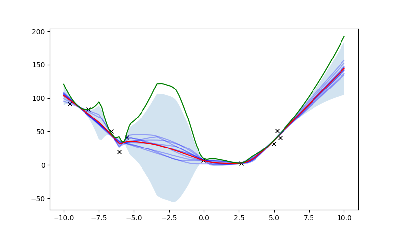
Key challenge: Distribution Shift

The policy optimizer can exploit the error in dynamics within out-of-distribution regime and result in very bad policy transfer.

1. First learn the dynamics of the system from data.

\begin{aligned} \min_\theta\quad & \mathbb{E}_\rho\left[{\color{red} V(x_0, \theta, \alpha)}\right] \\ & x_0 \sim \rho(x) \end{aligned}

Example Case: Model-Based Offline Policy Optimization

Previous Solutions:

\begin{aligned} \min_\theta\quad & \mathbb{E}_\rho\left[{\color{red} \mathbb{E}_\alpha V(x_0, \theta, \alpha)} + {\color{blue} \beta \text{Var}_\alpha V(x_0, \theta, \alpha)} \right] \\ \end{aligned}

Train Ensembles of dynamics where alpha is drawn from a finite set of distributions.

In addition to original cost, penalize quantified uncertainty (e.g. variance among ensembles).

\min_x \bigg[ {\color{green} f(x,\alpha) + \beta\text{Var}(f(x,\alpha))}\bigg]

\color{red} f(x)

\color{blue} f(x,\alpha)

Assumptions:

- High Variance among Ensembles implies OOD

- Ensembles can be trained successfully? (Glen might have complaints)

Proposed Method: Using direct training dist. prob.

Proposed Solution

\begin{aligned} \min_\theta\quad & \mathbb{E}_\rho\left[{\color{red} \mathbb{E}_\alpha V(x_0, \theta, \alpha)} + {\color{blue} \beta D(x_0, \theta))} \right] \\ \end{aligned}

Directly use our distribution risk

\begin{aligned} D(x_0, \theta) \coloneqq -\sum^{T-1}_{t=0} \log p(x_t, u_t) \end{aligned}

where p is obtained from our empirical distribution (training set).

Penalize horizontally as opposed to vertically

Some Benefits:

- Bypasses ensembles, pretty good since it's a sketchy uncertainty quantifier

- Minimum overhead, cheaper than ensemble.

Implicit Constraints on Data

What if we have some implicit constraints on data?

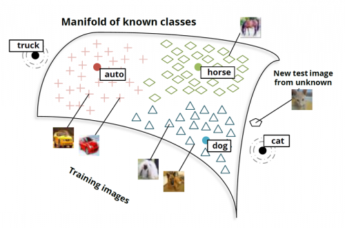
"The Manifold Hypothesis"

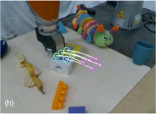
Rigid-Body Structure

\begin{aligned} x_{t+1} = f_\alpha(x_t, u_t) \end{aligned}

Wouldn't it be nice to able to constrain our dynamics to obey these constraints? What prevents these structure from being horribly violated after multiple rollouts?

Non-penetration Constraint

Distribution Risk as Imposition of Implicit Constraints

\begin{aligned} \min_\theta\quad & \mathbb{E}_\rho\left[c_T(x_T) + \sum^{T-1}_{t=0} c(x_t,u_t) - {\color{red} \beta\sum^{T-1}_{t=0} \log p(x_t,u_t)}\right] \\ \text{s.t.}\quad & x_{t+1} = f_\alpha(x_t, u_t) \;\; \forall t, \quad u_t = \pi_\theta(x_t, t)\;\;\forall t, \quad x_0 \sim \rho(x) \\ & {\color{blue} g(x_t,u_t) = 0} \end{aligned}

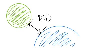
Claim: Let data lie on embedded submanifold M in the ambient space (x,u).

Denote denote the distance function (with the ambient space metric) between any (x,u) in the ambient space and the manifold M.

\begin{aligned} (x,u) \end{aligned}

\begin{aligned} g(x,u) \end{aligned}

Then, the negative log likelihood acts as a soft constraint penalizing deviation away from the submanifold M.

The Strict Case and Randomized Smoothing

If we were actually able to train p(x,u) in the limit of infinite data, we have:

\begin{aligned} -\log p(z) = \begin{cases} 0 & \text{ if } (z)\in\mathcal{M} \\ -\infty & \text{ else } \end{cases} \end{aligned}

So again, this corresponds to the case of requiring strict feasibility.

But such score models would be extremely hard to train. To get around this issue, score-based models utilize randomized smoothing:

\begin{aligned} z+w, \text{ where } z\sim p(z), \; w\sim\mathcal{N}(w;0,\mathbf{\Sigma}) \end{aligned}

\begin{aligned} z+w\sim \int p(z - w)\mathcal{N}(w; 0, \mathbf{\Sigma}) dw \end{aligned}

Gaussian Smoothing leads to Quadratic Penalty

\begin{aligned} -\log p(\bar{z}) & = - \log \exp\left[-\frac{1}{2}\|g(z)\|^2_{\mathbf{\Sigma}^{-1}}\right] \\ & = \frac{1}{2}\|g(z)\|^2_{\mathbf{\Sigma}^{-1}} \end{aligned}

To build some intuition, let's think of a simple case where p(x,u) is uniformly distributed on some manifold M.

The smoothed distribution is likely in the form of

\begin{aligned} \bar{z} = z+w\sim \mathcal{N}(g(z); 0, \mathbf{\Sigma}) \end{aligned}

Then, the negative log-likelihood is the penalty term of the constraint.

The general case is surprisingly hard to reason about!

Train a Generative Model of your Training Data,

Use it to fight Distribution Shift in Optimal Control