Funnel Progress

Recap of Problem

For some discrete-time system , find some tuple such that the policy stabilizes all to

It took a while to define what exactly the input/output portals refer to.

Attempt 1. Goal-conditioned Policies

\mathcal{S}_i,\mathcal{S}_f,\pi(\cdot;\cdot)

x'=f(x,u)

x_i\in\mathcal{S}_i

\pi(x ; x_f)

x_f

Challenges & Questions:

1. How do we get these goal-conditioned (a.k.a. universal) policies?

2. How do we represent these sets?

Attempt 1. Stochastic Policy Optimization (RL)

\begin{aligned} \min_\theta \quad & \mathbb{E}_{x_g\sim\mathcal{S}_g, x_i\sim \mathcal{S}_i}\left[\|x_T - x_g\|^2_\mathbf{Q} + \sum_t \|u_t\|^2_\mathbf{R} \right] \\ \text{s.t.} \quad & x_{t+1} = f(x_t, u_t) \quad \forall t \\ & u_t = \pi_\theta(x_t; x_g) \\ & x_0 = x_i \end{aligned}

In universal policy formulation, we can try to solve a stochastic policy optimization problem:

There is a chicken-and-egg problem between size of the sets and the ease of policy optimization.

1. How do we set the initial and goal sets? If they are too large, policy optimization is not

successful. Even if they are, there's no point since the whole point of our approach is to

decompose the problem into easier problems.

2. On the other hand, if they are too small, the resulting size of the graph is too large.

Attempt 1. Stochastic Policy Optimization (RL)

Performance of Policy Optimization with single goal

u_t = \mathbf{K}_t x_t + k_t

u_t = \pi_\theta(x_t)

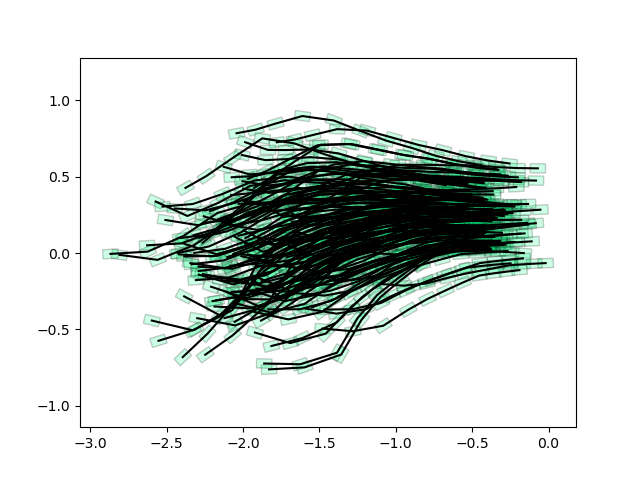
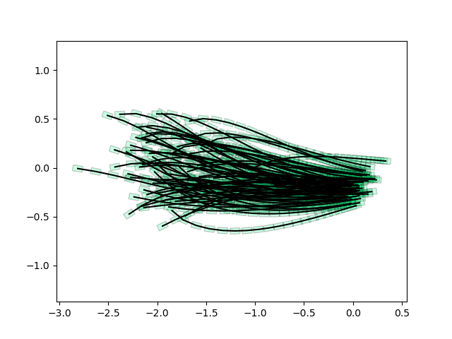
Policy with Time-varying gains and biases

Neural network policy

Not quite doing the job as well as I hoped.... Maybe because the initial set was not good?

Attempt 1. Stochastic Policy Optimization (RL)

Not quite doing the job as well as I hoped.... Maybe because the initial set was not good?

Iterative Refinement of the Initial Set

1. Solve the policy optimization problem from sample ellipsoid.

2. Perform weighted PCA on the initial set with weights

3. Sample from refined ellipsoid, repeat.

w(x^i_0) = \exp(-\alpha V(x^i_0))

Some factors led me to abandon this route.

1. Policy optimization is a bit costly to use as an inner routine in an alternation scheme.

2. At the same time, performance of PO was not that good when we care about reaching the goal exactly.

3. Many hyperparameters. How do we set reliably temperature parameter?

4. At the time, Pang was looking into LQR solutions with more promising results!

Re-usable Parts from this attempt.

\begin{aligned} \min_{\mathbf{K}_t,k_t} \quad & \left[\|x_T - x_g\|^2_\mathbf{Q} + \sum_t \|u_t\|^2_\mathbf{R} \right] \\ \text{s.t.} \quad & x_{t+1} = f(x_t, u_t) \quad \forall t \\ & u_t = \mathbf{K}_t x_t + k_t \\ & x_0 = x_i \end{aligned}

I have a pretty good single-shooting optimization algorithm for trajectory optimization!

\begin{aligned} \coloneqq V(\theta), \theta=(\mathbf{K}_t,k_t) \end{aligned}

Re-usable Parts from this attempt.

\begin{aligned} \nabla_{\theta} V(\theta) \end{aligned}

The solver supports three modes of estimating gradients

1. Policy Gradient Trick:

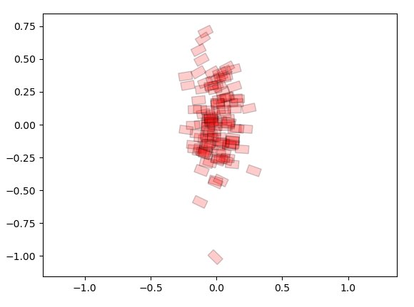
2. Autodiff computation graph with numerical gradients:

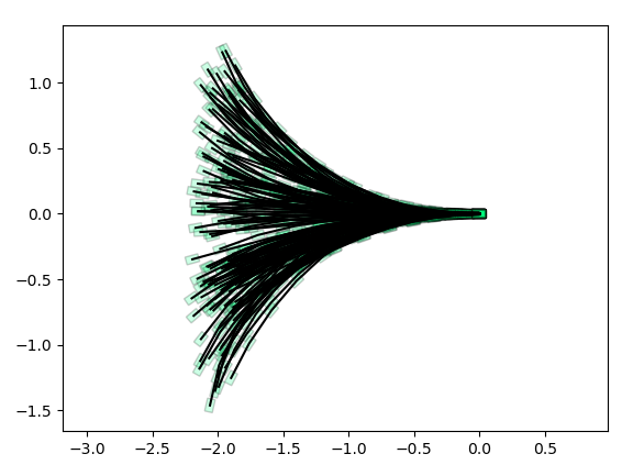
3. Autodiff computation graph with randomized gradients:

Inject Gaussian noise at output of the policy

w_t \sim \mathcal{N}(0,\sigma^2\mathbf{I})

\begin{aligned} \nabla_{\theta} \mathbb{E}_{w_t} [V(\theta)] = \frac{1}{\sigma^2} V(\theta) \sum^T_{t=0} \frac{\partial u_t}{\partial \theta}^\top w_t \end{aligned}

Do autodiff computations on the gradient, but approximate dynamic gradients with finite differences.

Do autodiff computations on the gradient, but approximate dynamic gradients with least-squares estimation of the gradient.

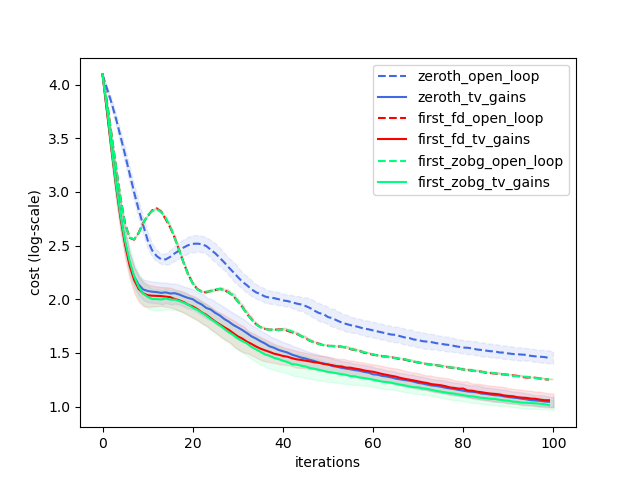
Trajopt Results

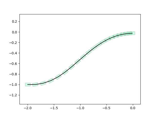
Trajopt significantly "easier" than policyopt, works quite reliably for now.

1. Having closed-loop gains to optimize makes a large difference in performance.

2. First-order optimizers more performant than the policy gradient trick.

Randomized vs. Finite Differences.

Attempt 2. Forwards Reachability

For some discrete-time system , find some tuple such that the policy stabilizes all to

Attempt 1. Goal-conditioned Policies

x'=f(x,u)

x_i\in\mathcal{S}_i

\pi(x ; x_f)

x_f

\mathcal{S}_i,\mathcal{S}_f,\pi(\cdot;\cdot)

Lessons: Directly optimizing for such policies is difficult. What if we don't ask for feedback-stabilizable set of goal points, but are willing to incorporate open-loop trajectories?

Attempt 2. Forwards Reachable Sets Robust to Disturbances on Initial Conditions

For some discrete-time system , given some set of initial conditions ,

Find where the definition is:

x'=f(x,u)

\mathcal{S}_f

\mathcal{S}_f = \{x_{T+1} | \exists u_0,\cdots,u_T \text{ with } \|u_t\|\leq \gamma \forall t \text{ for any } x_0 \in \mathcal{S}_i\}

x_i\in\mathcal{S}_i

Attempt 2. Robust Forward Reachable Sets

Forwards Reachable Sets Robust to Disturbances on Initial Conditions

For some discrete-time system , given some set of initial conditions ,

Find where the definition is:

x'=f(x,u)

\mathcal{S}_f

\mathcal{S}_f = \{x_{T+1} | \exists u_0,\cdots,u_T \text{ with } \|u_t\|\leq \gamma \forall t \text{ for any } x_0 \in \mathcal{S}_i\}

S_f = \cap_{x_0 \in \mathcal{S}_i} x_{T+1}(x_0)

Attempt 2. Robust Forward Reachable Sets

Specialization to Ellipsoids on LTV systems

\delta x_{t+1} = \mathbf{A}_t \delta x_t + \mathbf{B}_t \delta u_t

Set of finial conditions is characterized by Finite Impulse Response (FIR)

\delta x_{T+1} = \mathbf{N}\delta x_0 + \mathbf{M}_0 \delta u_0 + \mathbf{M}_1 \delta u_1 + \cdots \mathbf{M}_T \delta u_T

\|u_t\|^2\leq \gamma

If is zero, the reachable set under the constraint is given by

\{x_{T+1}\} = \mathcal{E}^\gamma_0 \oplus \mathcal{E}^\gamma_1 \oplus \cdots \oplus \mathcal{E}^\gamma_T

Suppose we solve trajopt for some nominal trajectory , and describe dynamics of disturbances with time-varying linearizations along this trajectory,

(x_0,\cdots,x_{T+1})

where .

\mathcal{E}^\gamma_t = \{x | x^\top \left[\mathbf{M}_t\mathbf{M}_t^\top\right]^{-1} x \leq \gamma \}

Note that this Minkowski sum results in a convex body with a unique minimum volume outer ellipsoid (MVOE), which can be solved with SDPs / Picard iterations. Denote this MVOE with .

\mathcal{E}^\gamma_{u}

\delta x_0

Attempt 2. Robust Forward Reachable Sets

What is we want to solve for nonzero disturbances?

\delta x_{T+1} = \mathbf{N}\delta x_0 + \mathbf{M}_u \delta u

\mathcal{E}^\gamma_{u} = \{x | x = \mathbf{M}_u \delta_u, \|\delta u\|\leq \gamma\}

Let denote parameters of the MVOE such that

\mathbf{M}_u, \delta_u

We can rewrite the FIR as a simple equation:

In addition, suppose that the uncertainty set for the initial condition is contained within some ellipsoid with quadratic form

\mathcal{E}^\rho_{x} = \{\delta x | \delta x^\top \mathbf{S} \delta x\leq \rho\}

What can we say about the set of such that there exists a point such that no matter what the adversary picks in , we can achieve ?

\delta x_{T+1}

x\in \mathcal{E}^\gamma_{u}

y \in \mathcal{E}^\rho_{\mathbf{A}x}

\delta x_{T+1} = x + y

\mathcal{E}^\rho_{\mathbf{A} x} = \{\delta x | \delta x^\top \mathbf{A}^{-\top}\mathbf{S}\mathbf{A}^{-1} \delta x\leq \rho\}

where we the image of this set through the linear map A becomes

Second Route: The Bottleneck Hypothesis

Intuition: Depending on the geometry, the intersection of all these cones for the reachable sets are necessarily bottlenecked around some location around the nominal trajectory.

Note that the true picture is far more complicated. x0 is an hyperellipsoid, and all time-slices of the cones are all hyperellipsoids.

Second Route: The Bottleneck Hypothesis

But these are far practical to compute if we fix a point.

x0: Backwards Reachable Set

Do TV-LQR along the red trajectory along its linearization, and determine ROA with line search.

x_{T+1}: Forward Reachable Set

Compute MVOE along the blue trajectory, already explained how to compute this given a fixed initial condition.

Bottleneck Hypoethesis: Suppose we fix a point and compute these forward / backward sets. Is there some initial region, rho, and gamma, such that this is the solution to the robust reachable sets problem?

Second Route: The Bottleneck Hypothesis

Backwards Reachable

Forwards Reachable

Intern Meeting