Differentiating through Discontinuities
Terry
Computing Gradients of Stochastic Objectives
Now let's talk about gradient computations.
Given that has differentiable almost everywhere but has jump discontinuities, how should we compute the gradient of the stochastic objective?
Quantity to compute / estimate:
Recall: The usual trick of D.C.T and Monte-Carlo doesn't work!
Back to our good old example....
Computing Gradients of Stochastic Objectives
We'll review three methods of how to resolve this.
- Use the zero-order numerical gradient.
- Bootstrap the function to a smooth function approximator.
- Analytically add back the Gaussian to the derivative.
Method 1.
If we use finite differences instead of gradients, the interval is not zero-measure, and will always be able to capture the discontinuity.
- Captures the behavior that we want nicely, but very difficult to analyze since we can't use Taylor.
- Usually suffers from higher variance, which leads to worse convergence rates.
Computing Gradients of Stochastic Objectives
Method 2. Bootstrapping to a smooth function approximator.
An effective solution, if you had lots of offline compute, is to simply find a differentiable representation of your discontinuous function by function fitting.
Computing Gradients of Stochastic Objectives
1. Evaluate the bundled objective at finite points:
2. Regress on e.g. neural network to find a surrogate function that is differentiable everywhere:
3. Compute the derivative of the surrogate function.
Doesn't "feel" right to me, but the learning people love this trick!
Bootstrapping to a smooth function approximator.
Computing Gradients of Stochastic Objectives
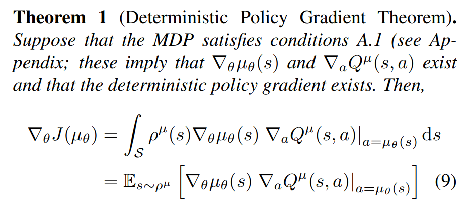
From DPG paper:
- If the Q function is discontinuous, won't they have the same issue?
- Not if they bootstrap a neural network to approximate Q!
Conv. w/ Abhishek
Likely, many learning methods bypass the problem with discontinuities by spending offline time to store discontinuities into continuous functions.
Of course, comes with some associated disadvantages as well.
Carrots example.
Computing Gradients of Stochastic Objectives
- Q: Why do we need neural simulators?
- A: Because we need gradients.
Conv. with Yunzhu:
Conv. with Russ:
- Q: Why don't you like the word "differentiable physics"?
- A: Physics has always been differentiable. Drake already gives you autodiff gradients through plant.
Resolution?
Perhaps gradients of the smooth representation of the plant can sometimes behave better than true plant gradients.
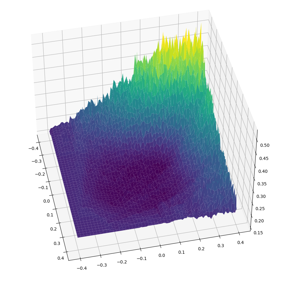
Very noisy landscape.
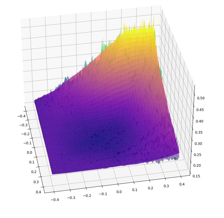
Bootstrapped to NN
Analytically adding back the Gaussian.
There is actually a quite easy solution to the delta issue if we really wanted to sample gradients....
Computing Gradients of Stochastic Objectives
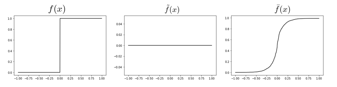
WLOG Let's represent the scalar function having discontinuities at x=0 as:
with
Then we can represent the gradient of the function as:
Gradient sampling fails because we have zero probability of landing at the delta
(and we can't evaluate it if we do anyways....)
Analytically adding back the Gaussian.
So instead of sampling the entire gradient, we can analytically integrate out the delta, then sample the rest.
Computing Gradients of Stochastic Objectives
Taken from "Systematically Differentiating Parametric Discontinuities", SIGGRAPH 2021.
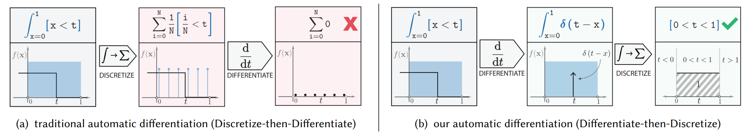
Analytically adding back the Gaussian.
So instead of sampling the entire gradient, we can analytically integrate out the delta, then sample the rest.
Computing Gradients of Stochastic Objectives
Decompose the integral into components without delta (top row), and the delta (bottom row).
Scaling to higher dimensions is challenging.
So how do we scale this to higher dimensions? Starts becoming real complicated....
Computing Gradients of Stochastic Objectives
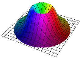
Derivative of heaviside is the delta, but what is the derivative of a 2D indicator function?
Does such a thing as make sense? Infinity at but ?
Consistent with the 1D delta? Many questions.
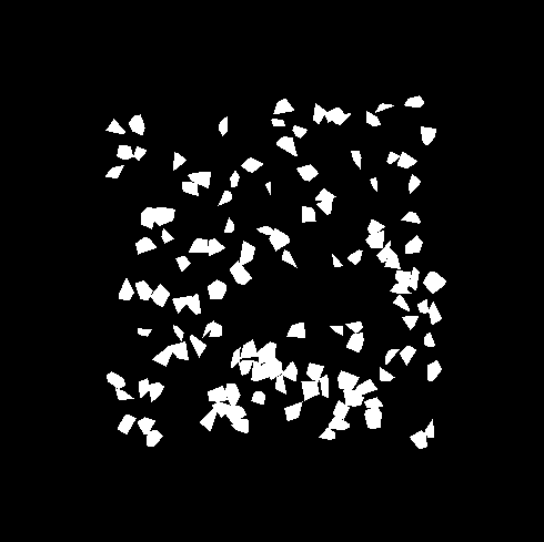
Convolution with 2D Gaussian gives a "ridge" of Gaussians,
Computational approach might be to find the closest surface of discontinuity, then evaluate the Gaussian centered at the closest point.