Randomized Smoothing
for Trajectory and Policy Optimization
Terry
Two Approaches to Optimal Control in Robotics
Differential Dynamics and Optimization
Tabular MDP and Approximate DP
Motivation: what explains the empirical success of RL methods? How do we "translate" what they did in a language that we (I) understand better, and use it for better performance? Is it the stochasticity? Is it the zero-order nature of their algorithms?
Deterministic
Rely on Analytical Gradients
Continuous State
Stochastic
Zero-order & Sampling
Discrete State
Robotics Problems
Nonlinear
Programming
Approximate Dynamic Programming
Robotics: Non-smooth, Non-convex Optimization
What are robotic problems? Why are they hard?
1. The optimal control problems are non-convex (and not gradient-dominant) - nonlinear dynamics.
2. The optimal control problems are non-smooth (contact, combinatorial choices).
3. Sometimes, optimal control problems can have discontinuities.
Problems in robotics are usually continuous state, reasonably deterministic problems.
We should expect to solve optimal control problems under such dynamics and costs with a deterministic policy. (i.e. there is nothing stochastic about the problem).
Deterministic, Non-convex, Non-smooth Problems.
Challenges in Differential Optimization: Nonconvexity
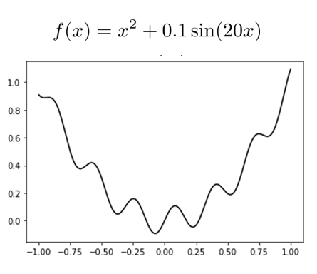
Non-convex (more precisely, not gradient dominant) functions can get you stuck in local minima
Often hinders good behavior in non-convex optimization:
Gradient is local (only looks at pointwise rate-of-change)
Trajopt for Car
Challenges in Differential Optimization: Non-smoothness
Gradient descent can be arbitrarily bad (even fail to converge to stationary points) for non-smooth problems.
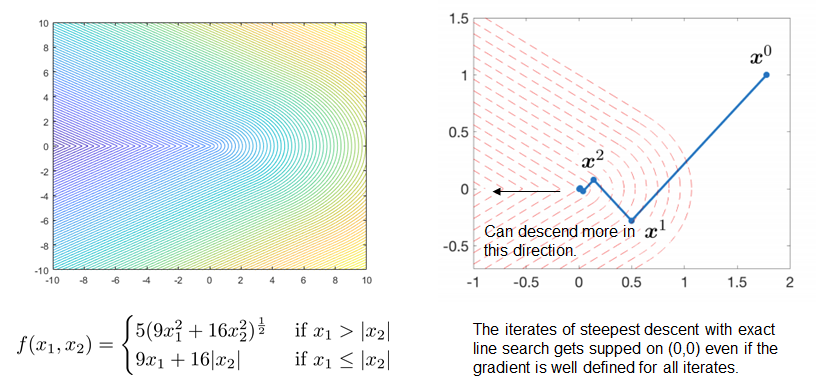
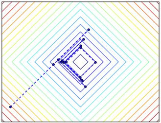
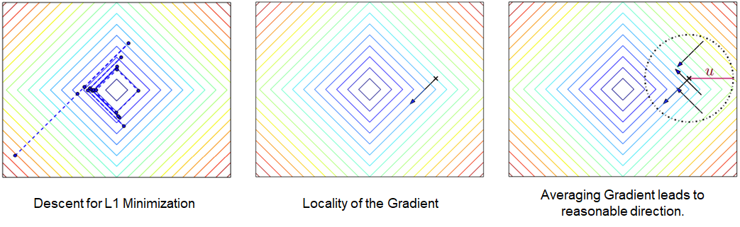
L1 minimization
Gradients in Robotics
The optimal control problems we solve in robotics are of non-convex, non-smooth nature.
But our tools behind typical optimization (SNOPT, etc.) are mostly gradient-based optimizers.
Natural that such solutions will be "fragile" (e.g. sensitive to initial guesses).
Robotics relies a lot on gradients....

Randomized Smoothing: Couple Insights
Randomized Smoothing
f is non-convex, potentially non-smooth. Not uncommon to have discontinuities. Hard to use gradients.
Introduce noise in the decision variables. How does this make the problem better?
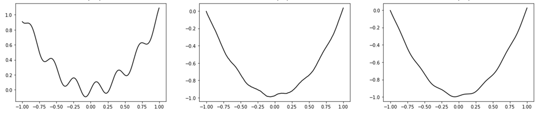
Original Objective
Surrogate Objective
Randomized Smoothing as Convolution
Convolution between original objective and the distribution.
- Smooths out high-frequency features of the cost to make the landscape nicer.
- Under choice of adequate kernels, convolution is guaranteed to be smooth.
- Lowers the Lipschitz constant of the resulting objective.
Gradient computation
Given information about , how do we compute the gradient of
Best case: we are given some analytical closed-form expression for , but highly unlikely.
Standard trick: Exchange expectation and derivative, then use Monte-Carlo to approximate expected value.
This is the "gradient sampling" algorithm - we can average a bunch of gradients and do descent with it, as opposed to the local gradient at the current iterate.
Failure Mode: Discontinuities
The algorithm has a particular failure case: functions with discontinuities.
Example: Consider Heaviside function.
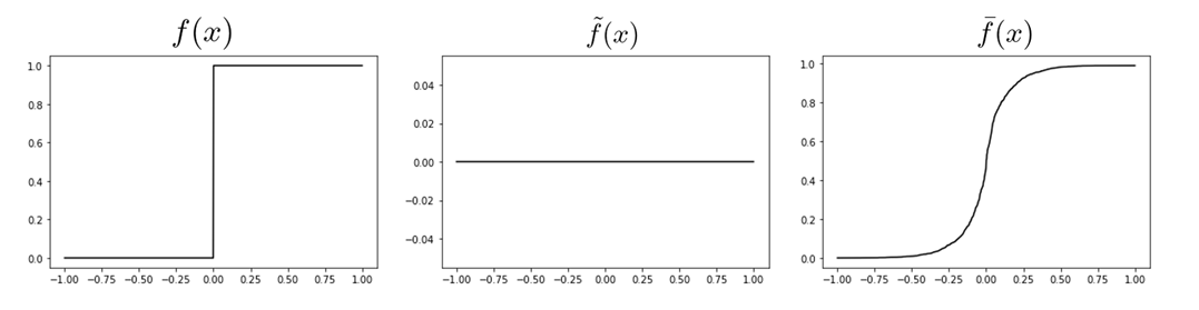
Staircase Effect in Non-smoothness
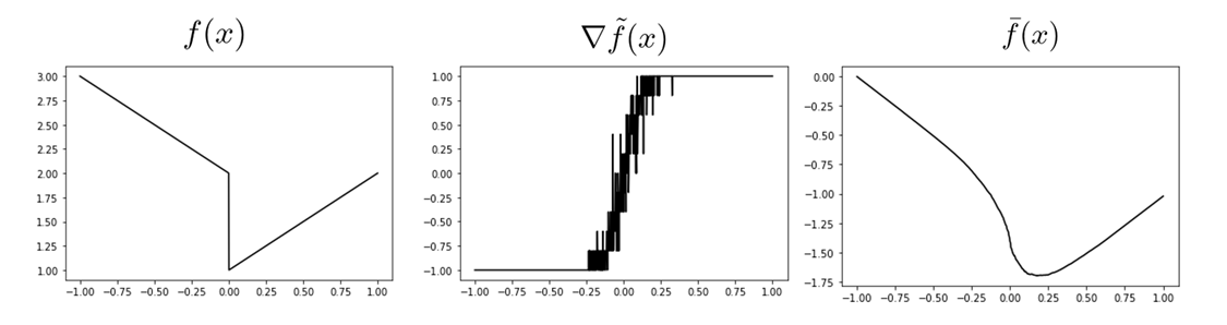
For non-smooth problems, can get a reasonable approximation.
But the quality of the approximation can be compromised in low-sample regimes.
(Staircase Effect)
Zero-order Variant
So how do we use randomized smoothing if the objective function is discontinuous?
One alternative is to take an expectation of finite differences instead:
1. Doesn't require f to be differentiable
2. More robust to numerics of discontinuities.
3. In fact, why should we use the gradient instead of the zero-order version, since we're sampling anyways?
Randomized Smoothing of the Value Function
Consider solving the following problem for deterministic initial condition and deterministic dynamics.
This setting covers the following problems:
- Open-loop policy optimization (i.e. trajectory optimization). Policy is simply parameterized as sequence of open-loop inputs.
- Closed-loop policy optimization from fixed initial state. (Typical policy optimization deals with expected value of this over multiple initial conditions)
Why might this problem be hard to tackle with typical gradients?
- Non-convexity of the optimization landscape (value function w.r.t. policy parameters).
- Non-smoothness that arises in some typical problems inherent in RL problems.
Toy Problem: Throwing Ball against the Wall
Back to high-school physics: suppose we throw a ball (Ballistic motion) and want to maximize the distance thrown using gradient descent.
Quiz: what is the optimal angle for maximizing the distance thrown?
Toy Problem: Throwing Ball against the Wall
Back to high-school physics: suppose we throw a ball (Ballistic motion) and want to maximize the distance thrown using gradient descent.
Quiz: what is the optimal angle for maximizing the distance thrown?
45 degrees!
If we plot the objective as a function of the angle, it is a nice gradient dominant function that will converge to the local minima.
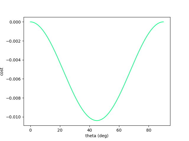
(Interestingly, this is non-convex. Typical example of one of Jack's PL inequality functions).
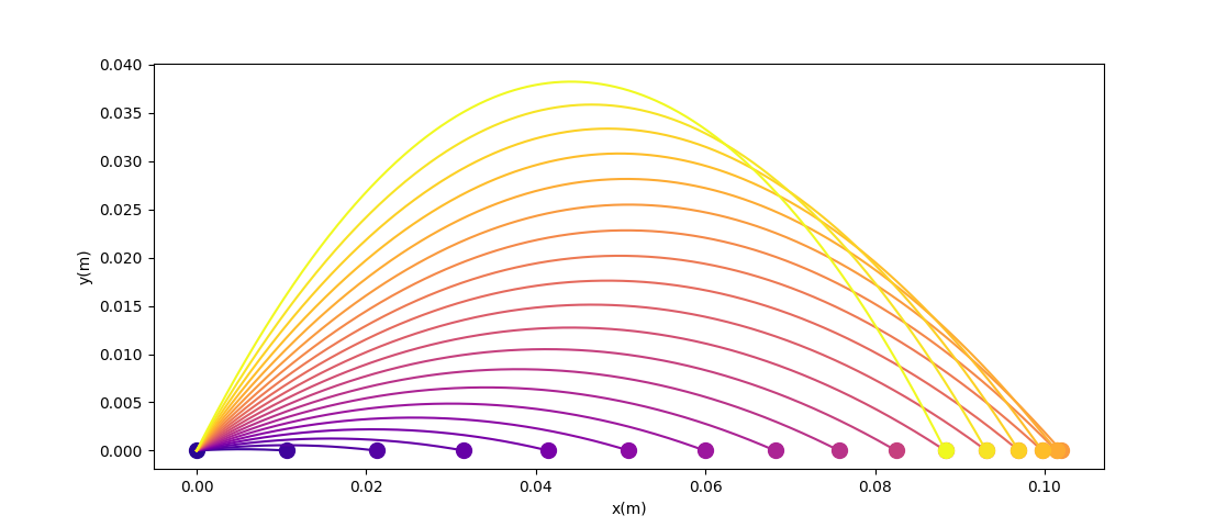
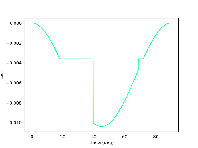
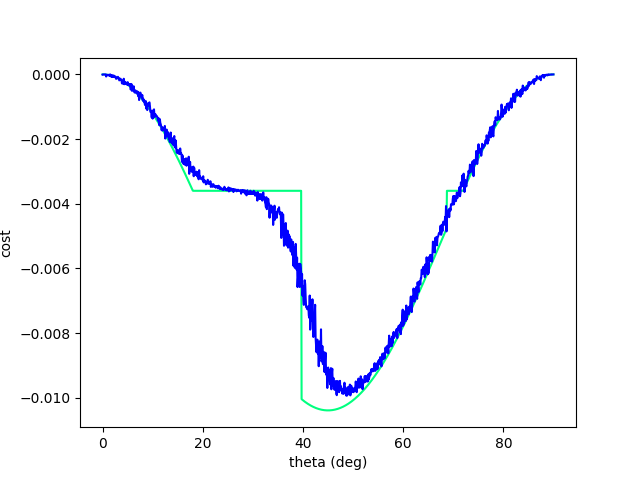
Toy Problem: Throwing Ball against the Wall
Back to high-school physics: suppose we throw a ball (Ballistic motion) and want to maximize the distance thrown using gradient descent.
Now we no longer have such nice structure....gradient descent fails.
There is fundamentally no local information to improve once we've hit the wall!
Even though the physical gradients are very well defined, we can no longer numerically obtain the minimum of the function.
Now let's add a wall to make things more interesting. (Assume inelastic collision with the wall - once it hits, falls straight down)

Randomized Smoothing to the Rescue.
Back to high-school physics: suppose we throw a ball (Ballistic motion) and want to maximize the distance thrown using gradient descent.
Now we have recover gradient dominance! Now we know where to go when we've hit the wall.
Note: there might exist an inflection point. But zero probability of landing there during gradient descent iterations?
To resolve this, consider a stochastic objective by adding noise to the decision variable:
Similar Examples: Lessons from Differentiable Sim.
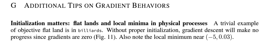
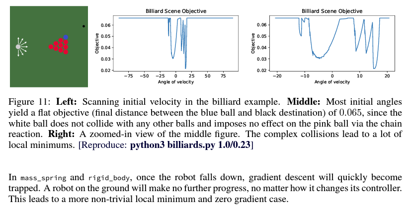
Excerpt from Difftaichi, one of the big diff. sims.
Rather surprising that we can tackle this problem with a randomized solution, without:
- manual tuning of initial guesses
- tree / graph search.
(Or rather, it was surprising to me at the beginning that gradients can't tackle this problem, the problem seems pretty easy and a search direction seems to exist.)
Some Connections
When are randomized policies better than deterministic policies?
The fact that you can obtain better performance with randomization in the presence of discontinuities is not new.
Binary Hypothesis Testing / Statistical Decision Theory (Neyman Pearson)
Deterministic Rules
Pareto Frontier
By randomizing, you can achieve better performance using the Neyman-Pearson criteria:
Danger of Gradient Strikes Again.
So we know that the stochastic objective is better for a more global search.
The problem is that we can no longer have a good way to utilize the gradient when the objective function is discontinuous.
Randomized Smoothing Policy Optimization
Note: In "Policy Optimization", we deal with optimization of closed-loop policy parameters.
Original Problem
Surrogate Problem
We think the surrogate problem has a nicer landscape compared to the original problem, w.r.t. two criteria:
- "Gradient dominance" of the landscape.
- Flatness / discontinuity of the gradients.
which suggests an algorithm to use the surrogate problem to better solve the original problem.
Sorry hold on!
Analytical Policy Gradient
Given the access to the following gradients:
One can use the chain rule to obtain the analytic gradients, that can be computed efficiently using autodiff on the rollout:
Conceivably, this can be used to update the parameters of the policy.
Policy Gradient Sampling Algorithm
Initialize some parameter estimate
While desired convergence:
Sample some initial states
Compute the analytical gradient of the value function from each sampled state.
Average the sampled gradients to obtain the gradient of the expected performance:
Update the parameters using gradient descent / Gauss-Newton.
Delta Strikes Again: Discontinuous Value Functions
Recall the following theorem: For discontinuous functions,
Recall the following theorem: For discontinuous functions,
We've previously looked at this in the context of contact dynamics, but the policy search suffers from similar problems.
But unlike contact dynamics (non-smooth but mostly continuous), the value function may truly suffer from many discontinuities.
Meaningful Question to ask: For which class of specifications / problems do we have discontinuous value functions?
- Could it appear for smooth systems in the presence of constraints?
- Viscosity solutions to the HJB equation: usually nonsmooth, but not quite discontinuous
- torque-limited pendulum (courtesy of Jack)
- Non-smoothness / Bifurcation in Dynamics
- Discontinuities in Cost
Zero-Order Policy Update
How do we solve the surrogate problem? Start with zero-order optimization.
Surrogate Problem
1. Sample the perturbations of the policy parameters.
2. Compute a direction of improvement w.r.t. policy parameters.
3. Update policy parameters with the computed direction.
4. Decrease the variance on injected noise as iterations converge.
Zero-Order Gradient Estimation (SPSA)
Randomized Smoothing Trajectory Optimization
Note: In "Trajectory Optimization", we deal with optimization of open-loop input sequences starting from a single initial point.
Original Problem (Single-shooting formulation)
Surrogate Problem
Note: Comparison with Previous Work
expectation over entire trajectory of noises
expectation over noise in a single timestep.
Question: how should we inject noise?
- Introducing noise of same variance at every timestep leads to extremely high variance estimates
- Least variance is when we take a deterministic policy up until the last step and sample the last action. However, such a solution does not smooth out the objective much.
- Adding noise in the beginning of the trajectory leads to large variance. However, it is most effective in exploring different possibilities.
- Fundamental tension between variance and exploration when optimizing for sequential decisions in open loop.
Variance Reduction vs. Exploration
Injecting noise right at the end of the trajectory will lead to a small variance among the distribution of value functions.
However, the capability to explore different solutions is extremely limited to a single timestep.
Injecting noise right at the front of the trajectory will lead to high variance among the distribution of value functions.
However, the method now has a lot of capability to explore. (Think of the ball throwing example)
What is the optimal way to trade off exploration vs. variance of the expected value function?
Perhaps we can reason about this in the space of increasing the width of the distribution for the latter part of the trajecotires.
Example:
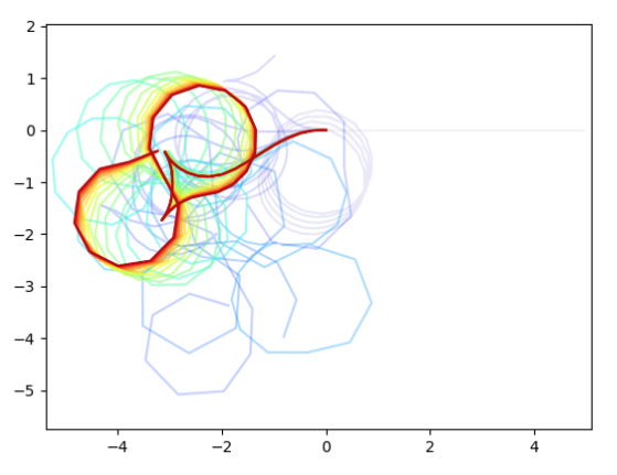
Randomized Smoothing Trajectory Optimization
We would like to use this for a more global exploration of contact modes.
Consider the following toy problem of pushing the box.
Goal configuration
Initial configuration
What we know about the problem:
-
Without any smoothing whatsoever, the gradient is zero. Unable to find good directions of improvement.
-
If we just smooth the dynamics and reason about the "bundled dynamics", cannot
Randomized Smoothing of Contact Dynamics
Smoothing of the Objective
Smoothing of the Dynamics
Questions, questions, and more questions.
1. What's the real tradeoff between analytical gradients (computed through symbolic / automatic diff), vs. numerical gradient? If there are considerable benefits to using analytical gradients (e.g. in higher dimensions), is there a way to modify the method for objectives with discontinuities?
2. What are useful questions for analysis? (Where do I go beyond the fact that this will "intuitively" help?) What are theoretical characterizations of performance (variance of the Monte-Carlo approximation? convergence rate?) under which cases?
3. Should we sample from the parameters, or append noise to the output?