Differentiable RL
Stream of Consciousness....
Policy Search Problem
Value Function
Initial distribution of rewards
Gaussian Policy
Deterministic & Differentiable Dynamics
Policy Optimization given Critic
Model Value Expansion
Suppose we have a estimate of our value function / Q-function.
Model-Based Component
Model-Free Component
DDPG
BPTT
Policy Optimization given Critic
Model Value Expansion
Suppose we have a estimate of our value function / Q-function.
Model-Based Component
Model-Free Component
DDPG
BPTT
Bias-Variance Tradeoff
Model Value Expansion
Suppose we have a estimate of our value function / Q-function.
Model-Based Component
Model-Free Component
- Unbiased in Expectation
- Potentially High Variance
- Biased Estimate
- Low Variance
Bias-Variance Tradeoff
Model Value Expansion
Suppose we have a estimate of our value function / Q-function.
Model-Based Component
Model-Free Component
- Unbiased in Expectation
- Potentially High Variance
- Biased Estimate
- Low Variance
Q1: How do we choose the horizon for a given system?
Horizon Selection
Model Value Expansion
Suppose we have a estimate of our value function / Q-function.
Model-Based Component
Model-Free Component
- Unbiased in Expectation
- Potentially High Variance
- Biased Estimate
- Low Variance
Consider a simple rule:
Horizon Selection
Model Value Expansion
Suppose we have a estimate of our value function / Q-function.
Model-Based Component
Model-Free Component
- Unbiased in Expectation
- Potentially High Variance
- Biased Estimate
- Low Variance
Consider a simple rule:
Maximize horizon to minimize bias
Until the variance is too difficult to handle
Controlling Model Variance
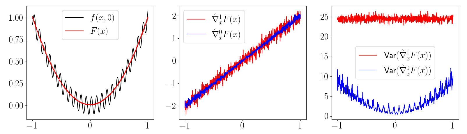
Variance Reduction
Can use empirical variance, but tend to be difficult to estimate.
Bound on First-order Gradient Variance given Lipschitz Constants
Controlling Dynamic Stiffness Alleviates Variance!
Controlling Model Variance
Variance Reduction
Can use empirical variance, but tend to be difficult to estimate.
Bound on First-order Gradient Variance given Lipschitz Constants
Controlling Dynamic Stiffness Alleviates Variance!
Less Stiff Dynamics Leads to Longer Model-Based Horizon
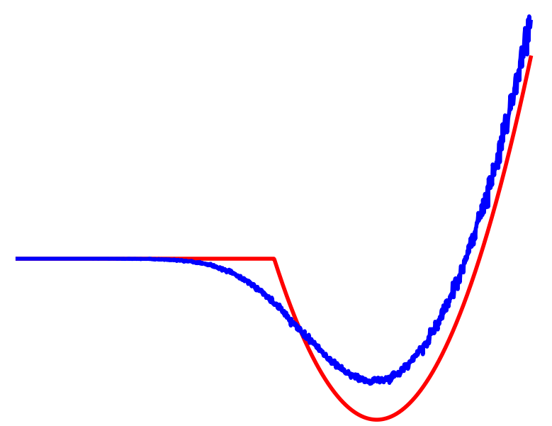
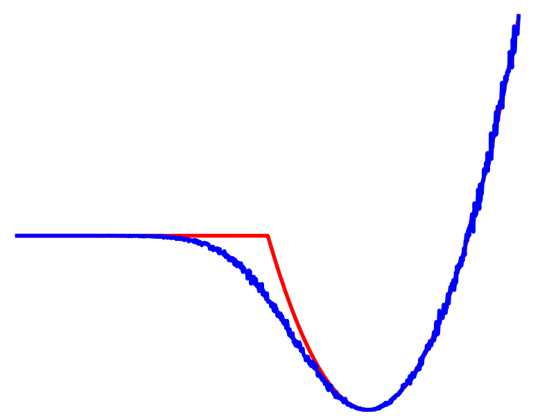
Dynamics Smoothing

Non-smooth Contact Dynamics
Smooth Surrogate Dynamics

No Contact
Contact
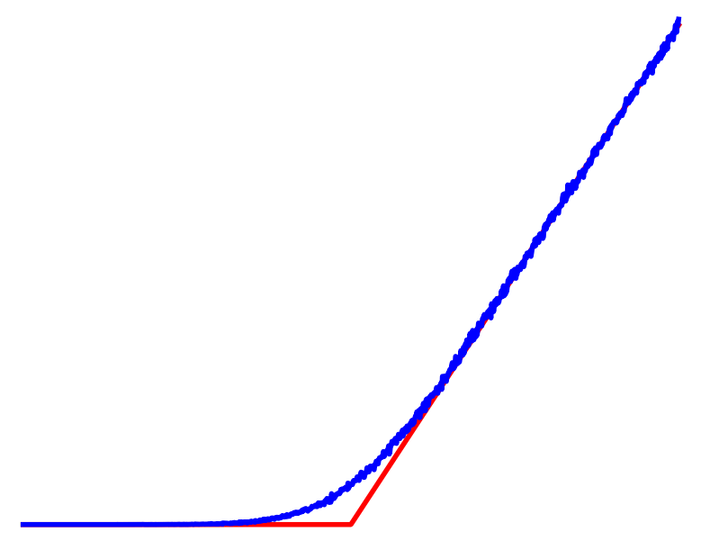
Averaged
Differentiable Simulator Comes with a Knob on Smoothness
Bias-Variance Tradeoff
Horizon Expansion
Dynamic Smoothing
High Gradient Estimation Variance
Low Gradient Estimation Bias
(Due to value estimation)
Low Gradient Estimation Variance
High Gradient Estimation Bias
(due to wrong dynamics)
Bias-Variance Tradeoff
Horizon Expansion
Dynamic Smoothing
High Dynamics Bias
Low Policy Gradient Variance
High Gradient Estimation Variance
Low Gradient Estimation Bias
(Due to value estimation)
Low Gradient Estimation Variance
High Gradient Estimation Bias
(due to wrong dynamics)
High Function Estimation Bias
Low Policy Gradient Variance
"The Path of Manageable Variance"
But how does annealing help?
If we only cared about low variance, might as well just run H=0 DDPG!
Does annealing help with value function estimation?
Reinforcement Learning
Cost
Contact
No Contact
Averaged
Dynamic Smoothing
Averaged
Contact
No Contact
No Contact
Previous analysis doesn't capture
dynamic smoothing benefits...
Dynamic Smoothing vs. Diffusion?
Score-based Generative Modeling
Policy Optimization through Contact
True data distribution lives on manifold, gradient is too stiff.
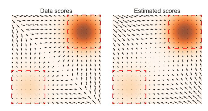
True contact dynamics is too stiff

Value Function Estimation
Model Value Expansion
Suppose we have a estimate of our value function / Q-function.
Model-Based Component
Model-Free Component
Q2: What's the right way to estimate the value,
1. Given that we will be using gradients,
2. Given that we chose some horizon H?
Bounding Gradient Bias
Original Problem (True Value)
Surrogate Problem
Gradient Bias (Quantity of Interest)
Bounding Gradient Bias
Gradient Bias (Quantity of Interest)
This part is unbiased
Bounding Gradient Bias
Gradient Bias (Quantity of Interest)
State Value Estimation
State-Action Value Estimation
Gradients need to match well over distribution of states at time t.
Push-forward measure from initial distribution under closed-loop dynamics
Bounding Gradient Bias
Gradient Bias (Quantity of Interest)
Usual Regression for Value Function Estimation
Sources of Bias
1. Distribution of data is from different behavior policy.
2. Accurate modeling of value does not guarantee modeling of gradients.
3. Bootstrapping bias.
Value Function Estimation
Finite-error modeling of value does not guarantee good gradients.
DDPG is equally questionable?
Value Gradient Boostrapping
Gradient Bias (Quantity of Interest)
State Value Estimation
In known dynamics case, suffices to estimate dV/dx well.
Value Gradient Boostrapping
Bellman Equation
Consider the boostrapping equation for TD(0)
Value Gradient Boostrapping
Bellman Equation
Consider the boostrapping equation for TD(0)
Bellman Gradient Equation
We can boostrap the gradient directly!
TD(k) Bootstrapping
Actor Loss
TD(k) Gradient Boostrapping (Critic Loss), can be weighted for TD Lambda
TD(k) Bootstrapping
TD(k) Gradient Boostrapping (Critic Loss), can be weighted for TD Lambda
Actor Loss
Critic H and Actor H does need not be the same!
Hypothesis: Actually it's beneficial to use the same H
1. Distribution of data is from different behavior policy.
2. Accurate modeling of value does not guarantee modeling of gradients.
3. Bootstrapping bias.
TD(k) Bootstrapping
Sources of Bias


TD(k) Gradient Boostrapping (Critic Loss), can be weighted for TD Lambda
Gradient Boostrapping Performance
Relies on Gradients from Models
High does dynamic stiffness affect estimation error?
TD(k) Gradient Boostrapping (Critic Loss), can be weighted for TD Lambda
Variance for long H and stiff dynamics tells us that
we should use less H for stiff dynamics!
Smoothing Conditioned Value Gradient
Critic Learning
Smoothing Conditioned Value Gradient
Actor Learning
Anneal H and rho simultaneously
(Noise Conditioned) Score Function under the
Control as Inference Interpretation
Differentiable Simulators
TinyDiffSim
gradSim
dFlex
Warp
Brax
Have my own preference on how I would implement it,
but not willing to go through the giant engineering time.
Mujoco FD
Personally have more trust in these,
but don't like soft contact models.