Updates with Russ

Parallelization of the iRS-LQR algorithm

Model Direcitive

iRS-LQR main thread

Worker t

Worker Pool (~30 threads)

Worker n

Sample over dynamics around single nominal point.

Each worker gets their own time segment of the trajectory to sample on.

Each worker gets their own time segment of the trajectory to sample on.

CPU parallelization can get good trajectories within seconds with Pang's quasistatic sim!

(~100 samples per knotpoint)

Successes Cases for Planning through Contact

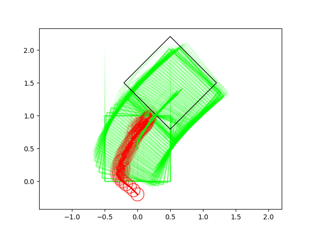
Box Pushing / Pivoting Examples

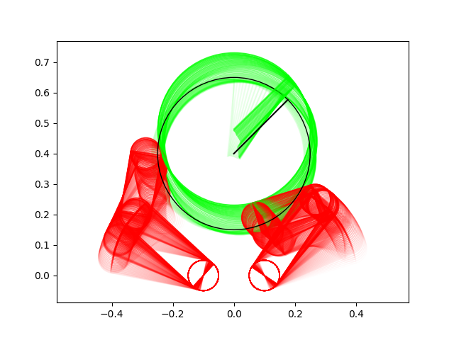
Planar In-hand Manipulation

Many of these results have very non-informative guesses as initial conditions.

(We really try not to avoid helping the algorithm in any way with initial guesses)

Most of the results so far use zero-order heavily.

Ball moving right

Ball moving left

Ball lifting

Ball rotation

Box trajectory tracking

Box pushing

Box pivoting w/ gravity

Box in-place rotation

The Importance of Randomized Smoothing

The exact method fails in cases where randomized smoothing succeeds. This seems to be because of the locality of the gradient for contact problems.

The Importance of Randomized Smoothing

• It is possible for the contact forces to be close to 0 in some multi-contact cases.

The Importance of Randomized Smoothing

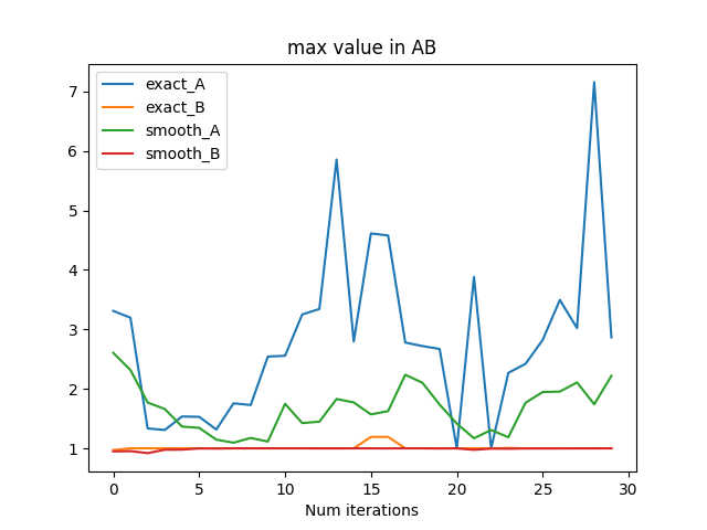
• When a contact has small contact force, the matrix we're inverting to compute the gradient of the dynamics is close to singular (left figure).
• This leads to large entries \(\hat{A}\) but not in \( \hat{B} \) (why?) (right figure).

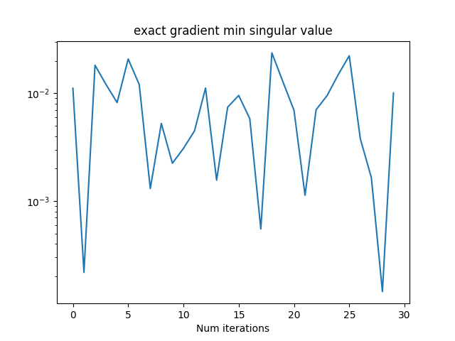
• Smoothing regularizes contact forces when the system is statically-indeterminate. Can we do that directly in the dynamics?

(should've plotted the condition number)

The Importance of Randomized Smoothing

• Larger entries in A lead to jerkier trajectories, and higher cost.

Exact gradient

Smoothed gradient

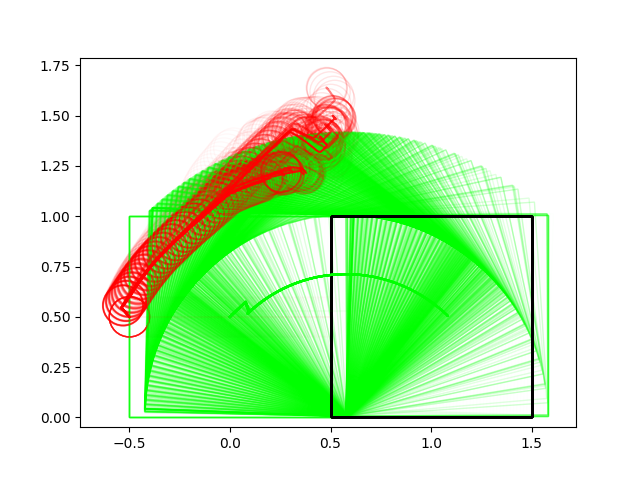
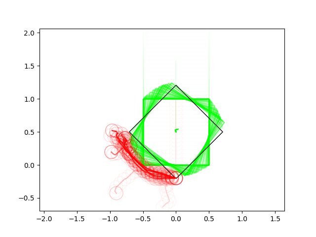
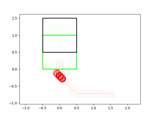
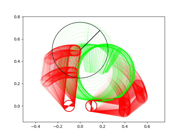
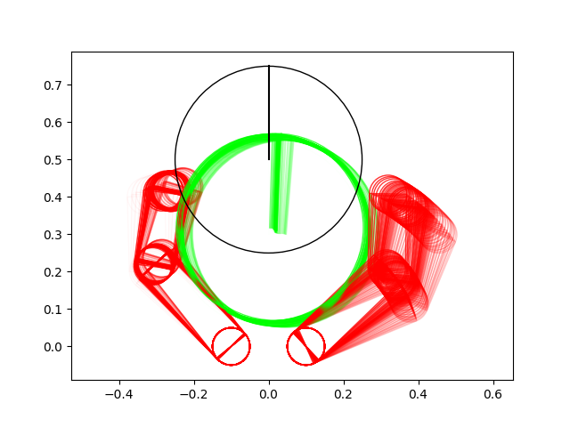
Failure Cases: Limitations of Local Optimization 

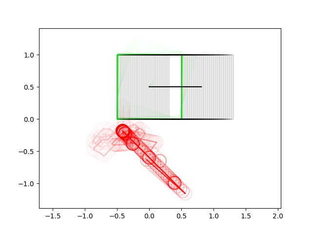
The algorithm doesn't realize it needs to go to the left of the box in order to produce the desired trajectory

The algorithm doesn't realize it needs to pinch the ball with the ends of fingers to lift the ball up

We promised some of our initial motivations was powering through some of these non-convexities of contact modes. So what's going on here?

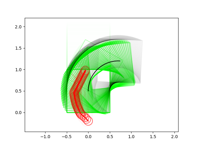
Failure Cases: Limitations of Local Optimization 

If we have to go to the other side, it requires knowledge that going to the other side is better (i.e. already requires value function across multiple initial conditions)

There is no "one-step" action that the pusher can take in order to realize it can do better by going to the left. In contrast, CEM will take that action sequence randomly and realize it decreases the cost, and slowly adjust.

Lesson 1. In order to power through non-convexities of long-horizon mode sequences, you really need to be taking expectations across trajectories, not one-step dynamics.

Lesson 2. For some problems, there is really no gap between planning from a single initial condition and getting a good policy across multiple initial conditions.

Failure Cases: Unstable descent behavior

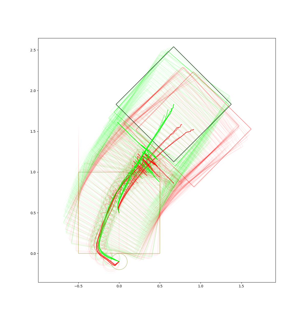
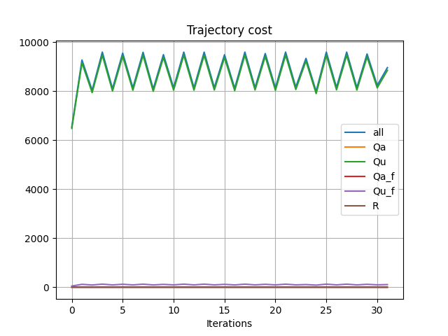
Lesson 3. Just like gradient descent and step sizes, the algorithm needs reasonable amount of tuning in order to get stable behavior. Accumulated many subtle tricks along the debugging process to stabilize iterations.

Red is even iterations, green is odd iterations.

Failure Cases: Numerical Ill-conditioning of Gradient

Fundamental tension between numerically well-conditioned gradients and accurate simulation of non-smooth contact!

Analysis: randomized smoothing of friction

We have sufficient understanding of what it's like to smooth out normal-direction contact forces for

Pang's position-controlled dynamics. Example: box-on-box dynamics is a ReLU, smoothing is softplus.

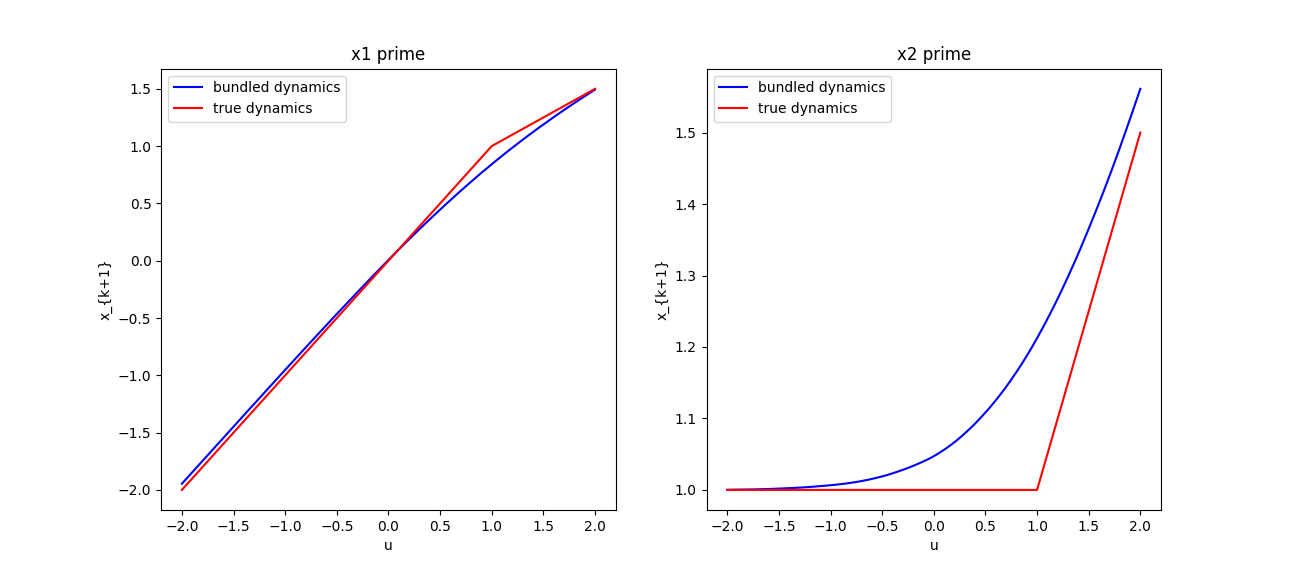
Analysis: randomized smoothing of friction

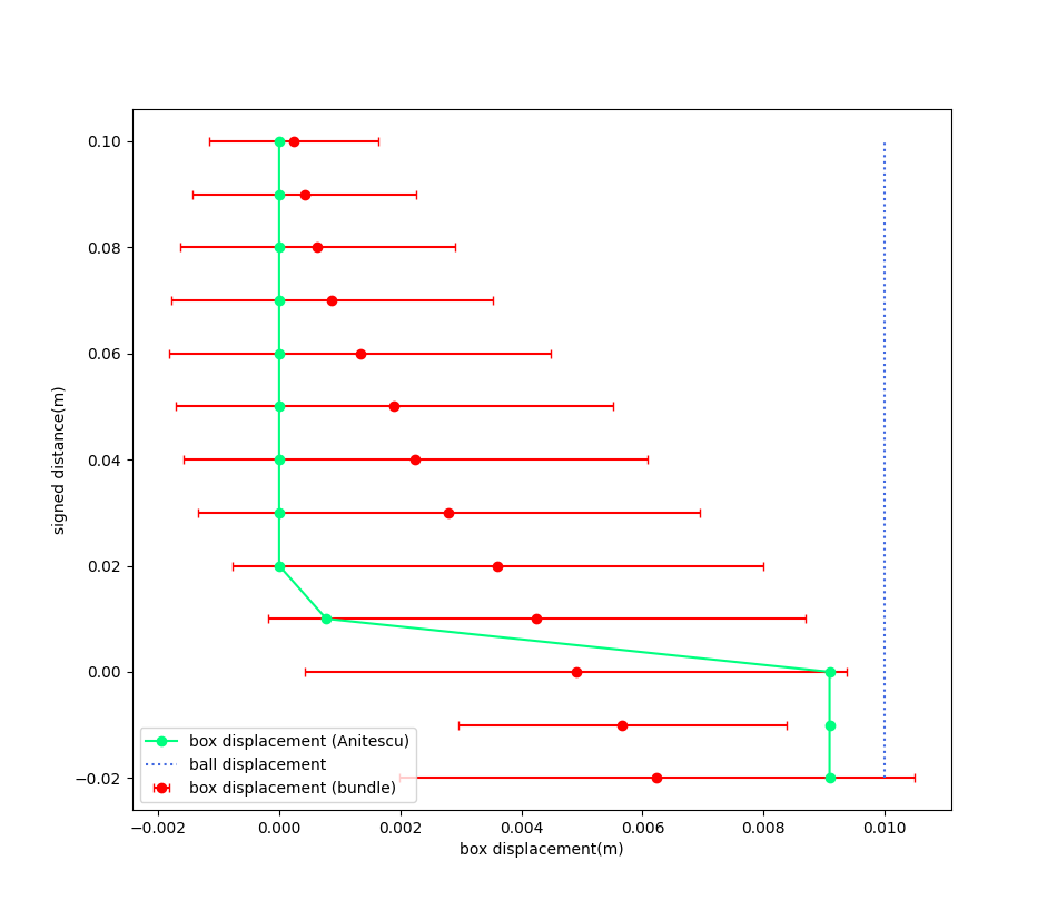
So what does randomized smoothing of friction look like? Not surprisingly, it imitates a boundary layer shaped like erfc. It drags the box in shear from a distance, and downplays the effect of friction when it is actually in contact.

Frictionless Surface

We move the ball in x by 0.01m, and vary the height between the box and the ball. The x-displacement of the box is plotted.

Box displacement under bundle dynamics

Box displacement under Anitescu

Displacement of the ball

Analysis: randomized smoothing of friction

But wait a minute....the Heaviside strikes back! We won't recover the bundle dynamics from first-order methods, but we can from zero-order methods. (We thought it was gone because the collision dynamics are ReLU)

Box displacement under bundle dynamics

Box displacement under Anitescu

Displacement of the ball

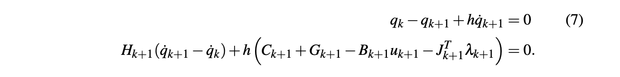
In the linearization, consider the change of x-coordinate of the box at the next timestep w.r.t. the y displacement of the ball.

Then, we get the conclusion that

The implication is that in the first order method, there is nothing telling the ball to go down in order to move the box, while the zero-order method retains this information.

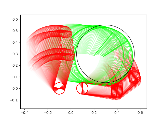
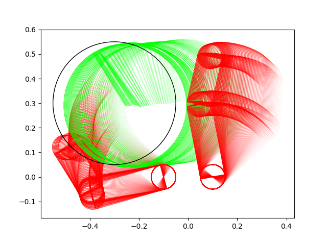
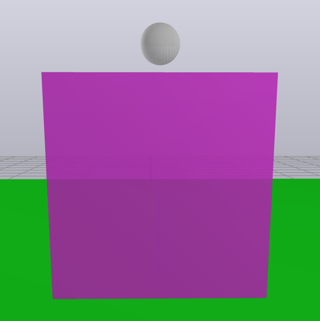
Back to Pang's gripper example

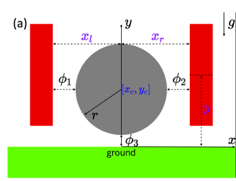
Rotate your head 90 degrees and we are back to the gripper problem. The gradient of the height of the ball w.r.t. the gripper gap is zero before and after contact, so nothing tells it to squeege the gripper in order to pull the ball upwards.

So what actually happens?

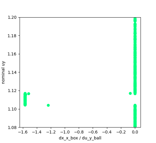
Contrary to the intuitive example, the first-order method still seems successful in predicting this gradient in code!

First order / Zero order Comparison of the B matrix estimated from sampling.

(We're plotting the sensitivity of dx_box w.r.t. dy_ball.)  

What's going on here? The first-order seems to have as good of an information as the zero-order method in predicting that it needs to go down to push the box!

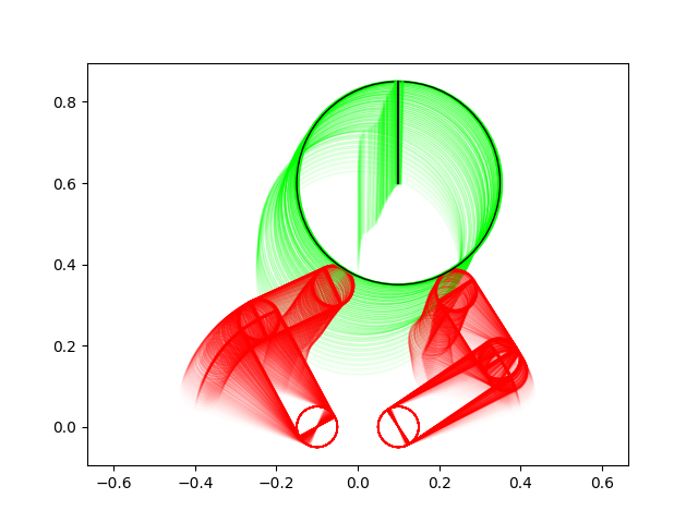
Anitescu saves the day for first-order method.

Anitescu's relaxation of the original LCP creates a boundary layer that inflates the delta function.

This somewhat saves the first order method from sampling from a delta function.

(We suspect similar things are saving people from running into this issue in Mujoco?)

Plot of gradient before sampling

dx_box / dy_ball (term in the B matrix)

zero before and after contact as we expected

But there is a "buffer zone"

Remaining Questions 

1. Do we have enough material to publish for RA-L? (September 9 deadline, ~2.7 weeks left)

2. How do we fit everything into 8 pages (Accumulated 2 pages of references at this point..)

3. What do you see as the main contribution of this work? Here is the story so far....

• Started out by saying we wanted to power through non-convexity of contact modes through expectation, this didn't quite work out as a strength (though we have examples where it powers through local minima)
• However, the prospect that zero-order optimization is just as powerful as first order optimization (even better in the presence of Heaviside, which you can't get away from in friction) is quite appealing.
• The fact that you can convert very gradient-dependent algorithms like iLQR into zero-order is quite appealing.
• Maybe all we need is a very fast parallelizable simulator instead of a differentiable one that we used to fixate on. (Maybe an argument for using LCP solvers instead of QPs?)

4. What are the remaining questions that we should be focusing on / what would you like to see more

• Empirical convergence / correctness behavior between first order, zero order, and exact gradient methods
• Effects of sample complexity (how does algorithm behave with more samples)
• More impressive examples?

TODO: More advanced examples

Big limitation comes from the difficulty of simulating multiple contacts at once