Smoothing Techniques for Optimal Control of Highly Contact Rich Systems
H.J. Terry Suh
MIT
Motivation: Why should we care?
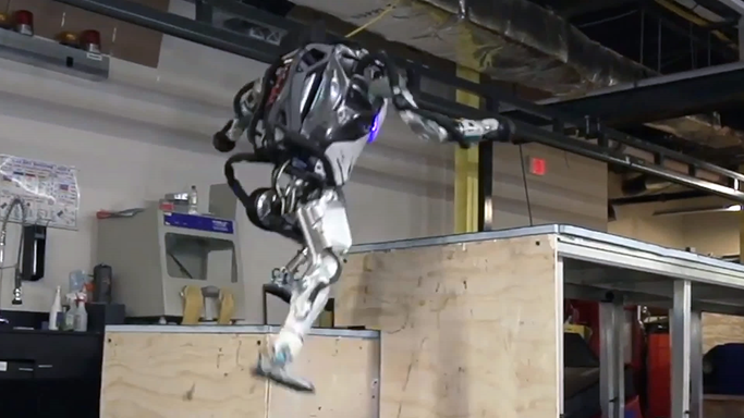
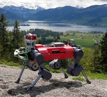
Agile & Autonomous Locomotion

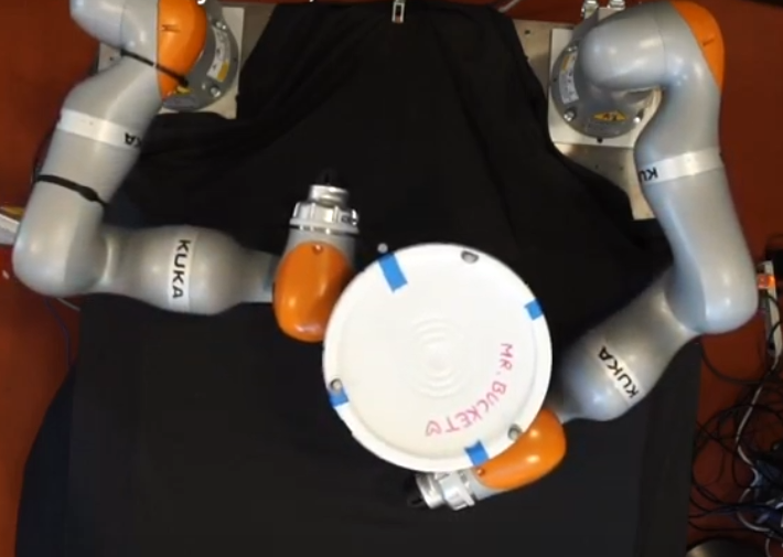
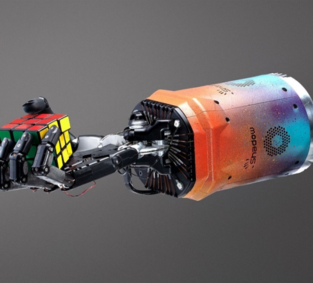
Dexterous Manipulation
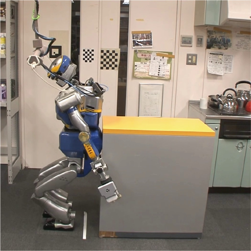
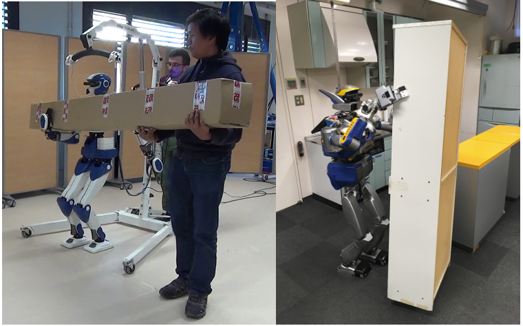
Whole-Body Loco-Manipulation
"The art of robots making contact where they are not supposed to make contact"
Motivation: What makes this problem difficult?
The Non-Smooth Nature of Contact makes tools from smooth optimization difficult to use.
Making & Breaking Contact
Non-smoothness of Friction
Non-smoothness of Geometry
Motivation: Hybrid Dynamics
Hybrid Dynamics
- Is appealing because it's a framework describes dynamical systems with mixed continuous and discrete variables.
- Divides the landscape into piecewise smooth regions, divided by manifolds that cause non-smoothness.
- General solutions to optimal control of hybrid dynamics involve having to decide which of these pieces to choose, while optimizing within each individual piece. (Mixed-Integer Nonlinear Programming)
Motivation: The Fallacy of Hybrid Dynamics
Contact is non-smooth. But Is it truly "discrete"?
The core thesis of this talk:
Counting contact modes for these kinds of systems results in trillions of modes.
Are we truly thinking of whether we're making contact or not for all possible fingers?
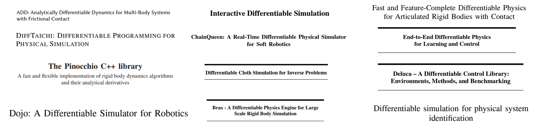
Smoothing Techniques for Non-Smooth Problems
Some non-smooth problems are successfully tackled by smooth approximations without sacrificing much from bias.
Is contact one of these problems?
*Figures taken from Yuxin Chen's slides on "Smoothing for Non-smooth Optimization"
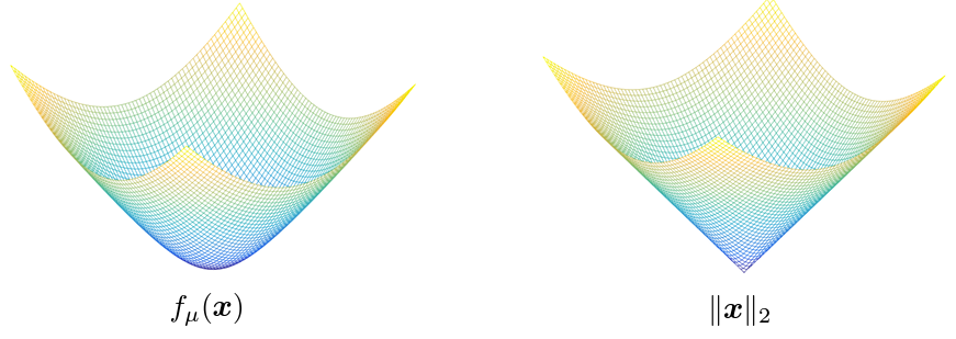
Smoothing in Optimization
We can formally define smoothing as a process of convolution with a smooth kernel,
In addition, for purposes of optimization, we are interested in methods that provide easy access to the derivative of the smooth surrogate.
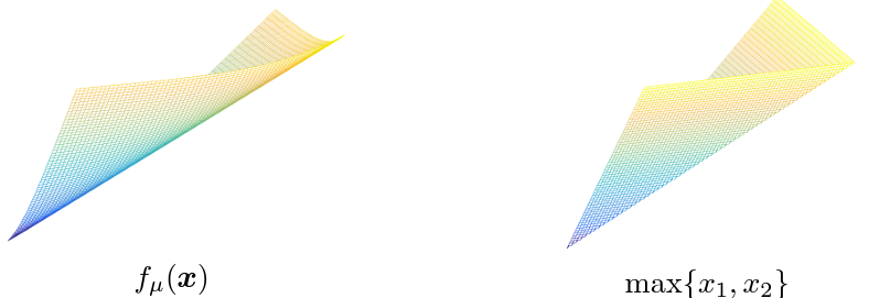
Original Function
Smooth Surrogate
Derivative of the Smooth Surrogate:
These provide linearization Jacobians in the setting when f is dynamics, and policy gradients in the setting when f is a value function.
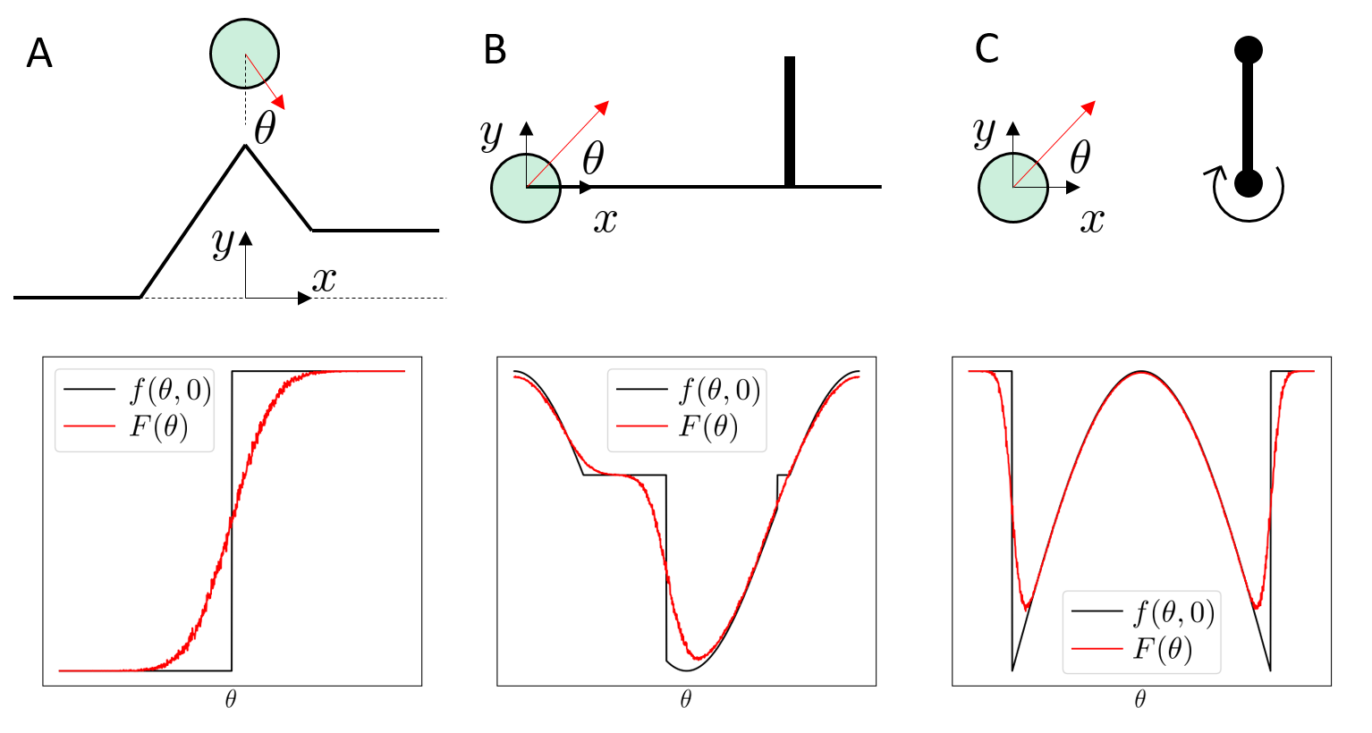
Taxonomy of Smoothing
Case 1. Analytic Smoothing
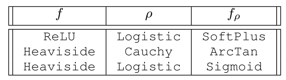
- If the original function f and the distribution rho is sufficiently structured, we can also evaluate the smooth surrogate in closed form by computing the integral.
- This can be analytically differentiated to give the derivative.
- Commonly used in ML as smooth nonlinearities.
Taxonomy of Smoothing
Case 2. Randomized Smoothing, First Order
- When we write convolution as an expectation, it motivates Monte-Carlo sampling methods that can estimate the value of the smooth surrogate.
- In order to obtain the derivative, we can use the Leibniz integral rule to exchange the expectation and the derivative.
- This means we can sample derivatives to approximate the derivative of the sampled function.
- Requires access to the derivative of the original function f.
- Also known as the Reparametrization (RP) gradient.
Taxonomy of Smoothing
Case 2. Randomized Smoothing, First Order
*Figures taken from John Duchi's slides on Randomized Smoothing
Taxonomy of Smoothing
Case 2. Randomized Smoothing, Zeroth-Order
- Interestingly, we can obtain the derivative of the randomized smoothing objective WITHOUT having access to the gradients of f.
- This gradient is derived from Stein's lemma
- Known by many names: Likelihood Ratio gradient, Score Function gradient, REINFORCE gradient.
This seems like it came out of nowhere? How can this be true?
Taxonomy of Smoothing
Rethinking Linearization as a Minimizer.
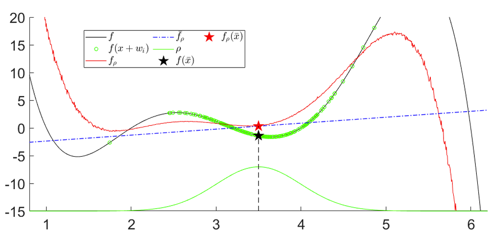
- The linearization of a function provides the best linear model (i.e. up to first order) to approximate the function locally.
- We could use the same principle for a stochastic function.
- Fix a point xbar. If we were to sample bunch of f(xbar + w_i) and run a least-squares procedure to find the best linear model, this converges to the linearization of the smooth surrogate.
Also provides a convenient way to compute the gradient in zeroth-order. Just sample and run least-squares!
Tradeoffs between structure and performance.
The generally accepted wisdom: more structure gives more performance.
Analytic smoothing
Randomized Smoothing
First-Order
Randomized Smoothing
Zeroth-Order
- Requires closed-form evaluation of the integral.
- No sampling required.
- Requires access to first-order oracle (derivative of f).
- Generally less variance than zeroth-order.
- Only requires zeroth-order oracle (value of f)
- High variance.
Structure Requirements
Performance / Efficiency
Smoothing of Contact Dynamics
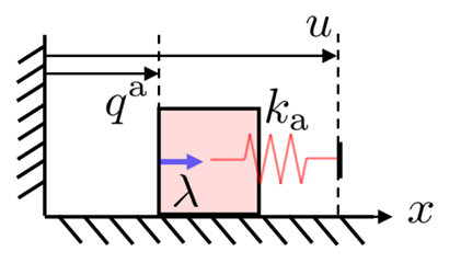
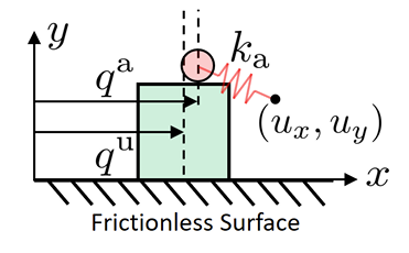
Without going too much into details of multibody contact dynamics, we will use time-stepping, quasidynamic formulation of contact.
- We assume that velocities die out instantly
- Inputs to the system are defined by position commands to actuated bodies.
- The actuated body and the commanded position is connected through an impedance source k.
Equations of Motion (KKT Conditions)
Non-penetration
(Primal feasibility)
Complementary slackness
Dual feasibility
Force Balance
(Stationarity)
Quasistatic QP Dynamics
We can randomize smooth this with first order methods using sensitivity analysis or use zeroth-order randomized smoothing.
But can we smooth this analytically?
Barrier (Interior-Point) Smoothing
Quasistatic QP Dynamics
Equations of Motion (KKT Conditions)
Interior-Point Relaxation of the QP
Equations of Motion (Stationarity)
Impulse
Relaxation of complementarity
"Force from a distance"
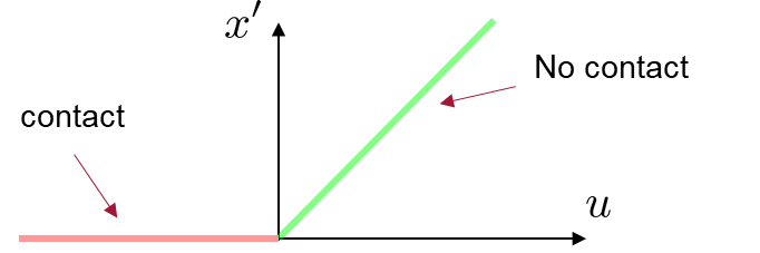
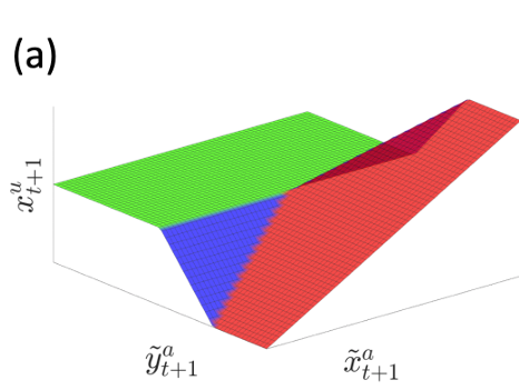
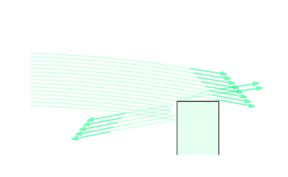
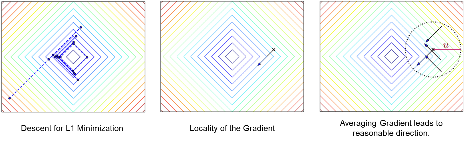
What does smoothing do to contact dynamics?
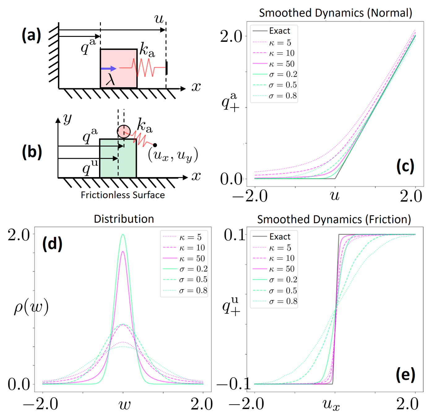
- Both schemes (randomized smoothing and barrier smoothing) provides "force from a distance effects" where the exerted force increases with distance.
- Provides gradient information from a distance.
- In contrast, without smoothing, zero gradients and flat landscapes cause problems for gradient-based optimization.
Is barrier smoothing a form of convolution?
Equivalence of Randomized and Barrier Smoothing.
- For the simple 1D pusher system, it turns out that one can show that barrier smoothing also implements a convolution with the original function and a kernel.
- This is an elliptical distribution with a "fatter tail" compared to a Gaussian".
Later result shows that there always exists such a kernel for Linear Complementary Systems (LCS).
Optimal Control with Dynamics Smoothing
Replace linearization in iLQR with smoothed linearization
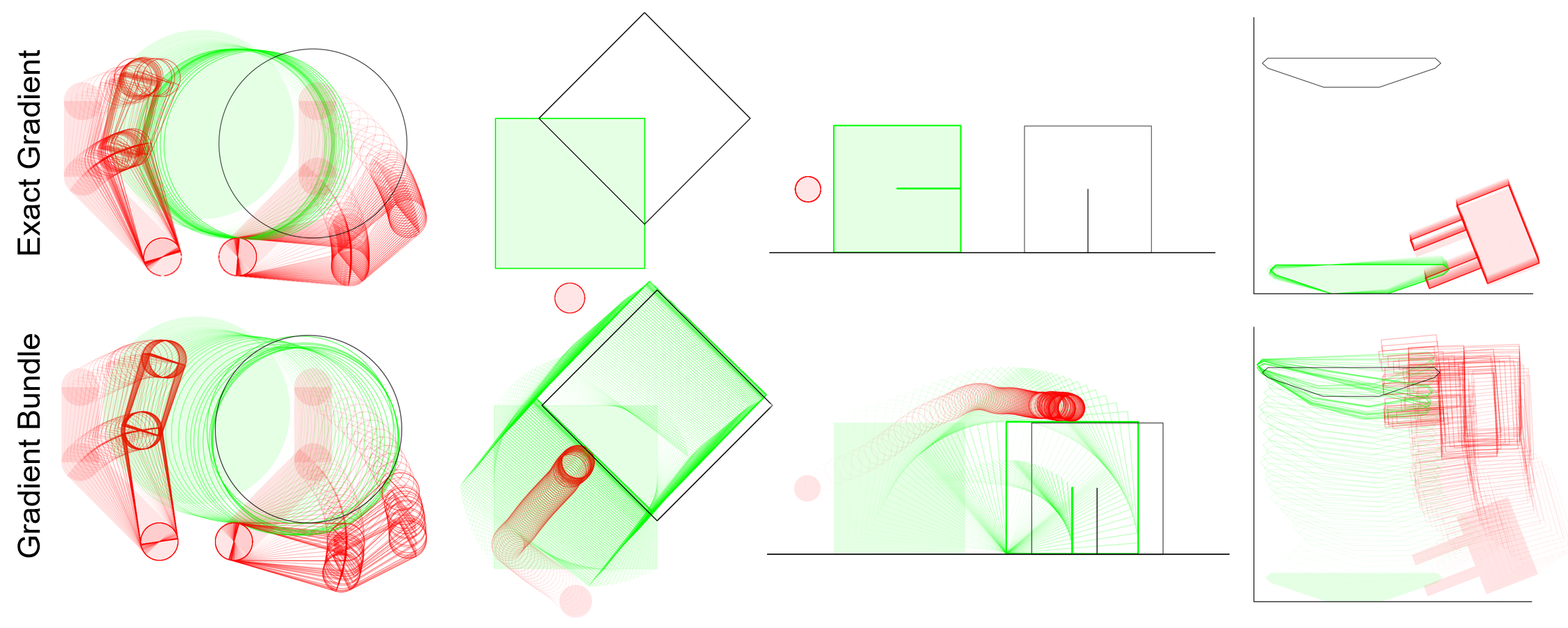
Exact
Smoothed
Smoothing of Value Functions.
Optimal Control thorugh Non-smooth Dynamics
Policy Optimization
Cumulative Cost
Dynamics
Policy (can be open-loop)
Dynamics Smoothing
Value Smoothing
Recall that smoothing turns into .
Why not just smooth the value function directly and run policy optimization?
Smoothing of Value Functions.
Original Problem
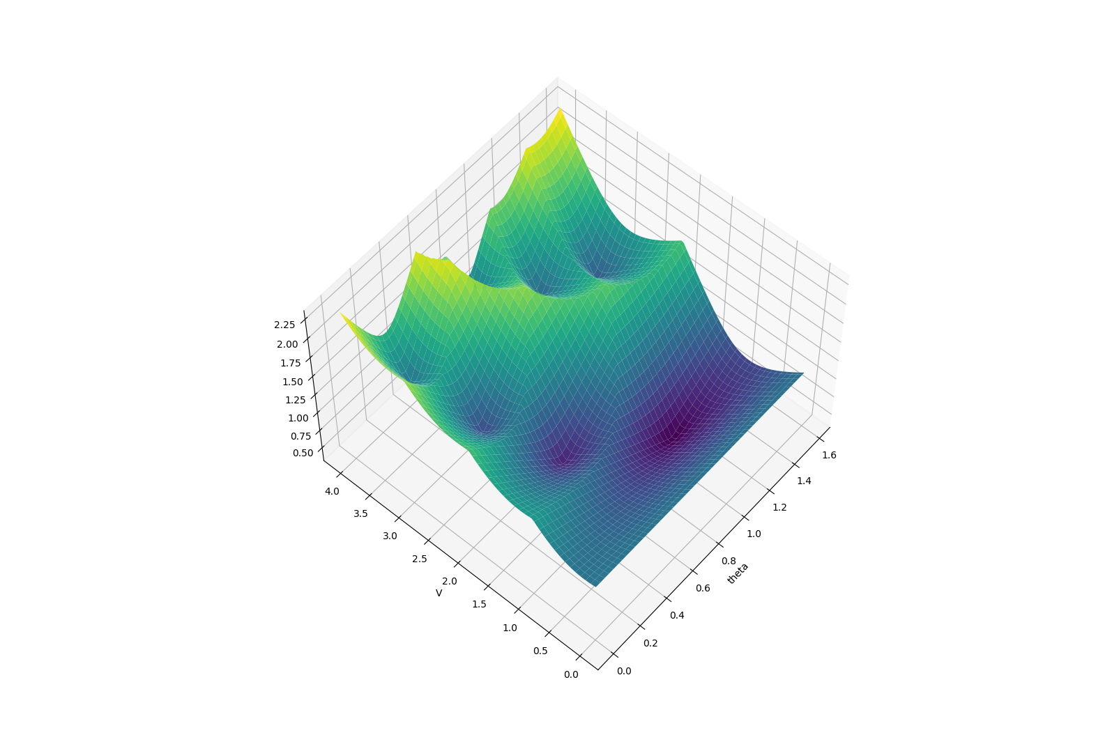
Long-horizon problems involving contact can have terrible landscapes.
Smoothing of Value Functions.
Smooth Surrogate
The benefits of smoothing are much more pronounced in the value smoothing case.
Beautiful story - noise sometimes regularizes the problem, developing into helpful bias.
How do we take gradients of smoothed value function?
Analytic smoothing
Randomized Smoothing
First-Order
Randomized Smoothing
Zeroth-Order
- Requires differentiability over dynamics, reward, policy.
- Generally lower variance.
- Only requires zeroth-order oracle (value of f)
- High variance.
Structure Requirements
Performance / Efficiency
Pretty much not possible.
How do we take gradients of smoothed value function?
First-Order Policy Search with Differentiable Simulation
Policy Gradient Methods in RL (REINFORCE / TRPO / PPO)
- Requires differentiability over dynamics, reward, policy.
- Generally lower variance.
- Only requires zeroth-order oracle (value of f)
- High variance.
Structure Requirements
Performance / Efficiency
Turns out there is an important question hidden here regarding the utility of differentiable simulators.
Do Differentiable Simulators Give Better Policy Gradients?
Very important question for RL, as it promises lower variance, faster convergence rates, and more sample efficiency.
What do we mean by "better"?
Consider a simple stochastic optimization problem
First-Order Gradient Estimator
Zeroth-Order Gradient Estimator
Then, we can define two different gradient estimators.
What do we mean by "better"?
First-Order Gradient Estimator
Zeroth-Order Gradient Estimator
Bias
Variance
Common lesson from stochastic optimization:
1. Both are unbiased under sufficient regularity conditions
2. First-order generally has less variance than zeroth order.
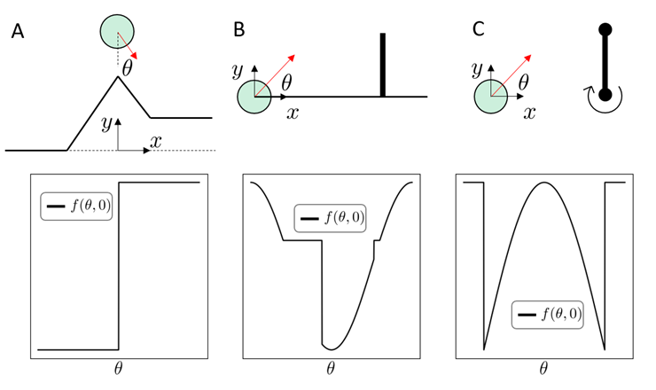
What happens in Contact-Rich Scenarios?
Bias
Variance
Common lesson from stochastic optimization:
1. Both are unbiased under sufficient regularity conditions
2. First-order generally has less variance than zeroth order.
Bias
Variance
Bias
Variance
We show two cases where the commonly accepted wisdom is not true.
1st Pathology: First-Order Estimators CAN be biased.
2nd Pathology: First-Order Estimators can have MORE
variance than zeroth-order.
Bias from Discontinuities
1st Pathology: First-Order Estimators CAN be biased.
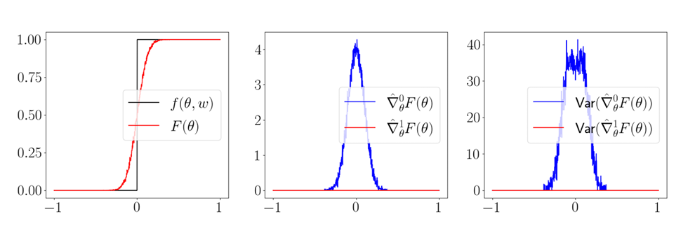
What's worse: the empirical variance is also zero!
(The estimator is absolutely sure about an estimate that is wrong)
Not just a pathology, could happen quite often in contact.
Empirical Bias leads to High Variance
Perhaps it's a modeling artifact? Contact can be softened.
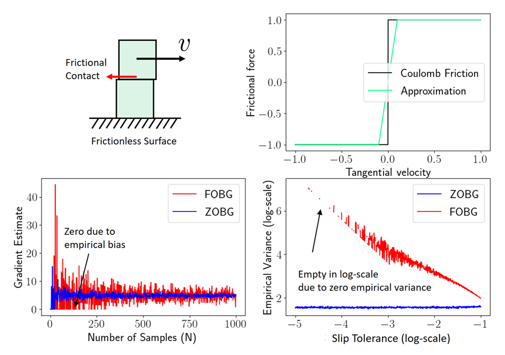
- From a low-sample regime, no statistical way to distinguish between an actual discontinuity and a very stiff function.
- Generally, stiff relaxations lead to high variance. As relaxation converges to true discontinuity, variance blows up to infinity, and suddenly turns into bias!
- Zeroth-order escapes by always thinking about the cumulative effect over some finite interval.
Variance of First-Order Estimators
2nd Pathology: First-order Estimators CAN have more variance than zeroth-order ones.
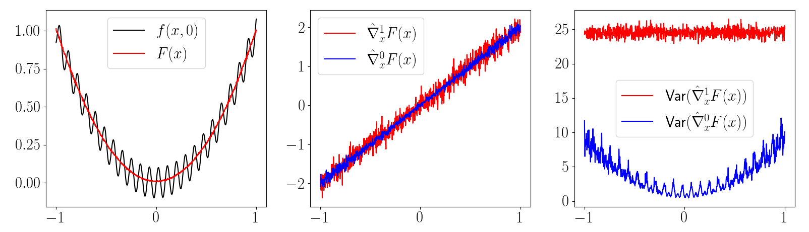
Scales with Gradient
Scales with Function Value
Scales with dimension of decision variables.
High-Variance Events
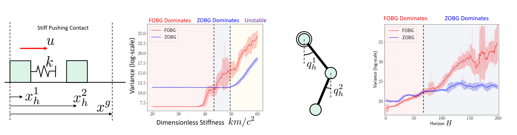
Case 1. Persistent Stiffness
Case 2. Chaotic
- Contact modeling using penalty method is a bad idea for differentiable policy search
- Gradients always has the spring stiffness value!
- High variance depending on initial condition
- Zeroth-order always bounded in value, but the gradients can be very high.
Motivating Gradient Interpolation
Bias
Variance
Common lesson from stochastic optimization:
1. Both are unbiased under sufficient regularity conditions
2. First-order generally has less variance than zeroth order.
Bias
Variance
Bias
Variance
1st Pathology: First-Order Estimators CAN be biased.
2nd Pathology: First-Order Estimators can have MORE
variance than zeroth-order.
Can we automatically decide which of these categories we fall into based on statistical data?
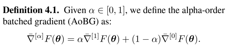
The Alpha-Ordered Gradient Estimator
Perhaps we can do some interpolation of the two gradients based on some criteria.
Previous works attempt to minimize the variance of the interpolated estimator using empirical variance.
Robust Interpolation
Thus, we propose a robust interpolation criteria that also restricts the bias of the interpolated estimator.
Robust Interpolation
Robust Interpolation
Implementation
Confidence Interval on the zeroth-order gradient.
Difference between the gradients.
Key idea: Unit-test the first-order estimate against the unbiased zeroth-order estimate to guarantee correctness probabilistically. .
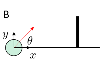
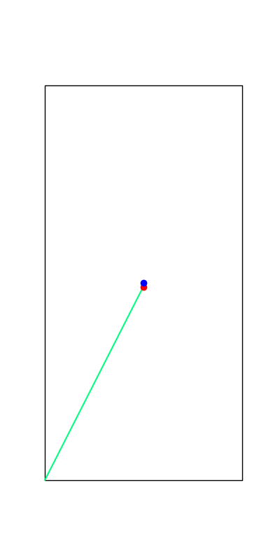
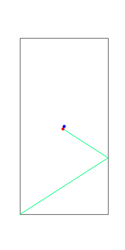
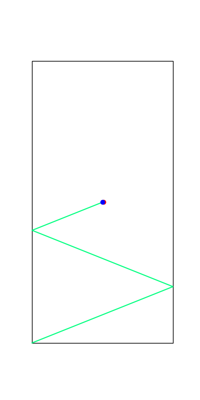
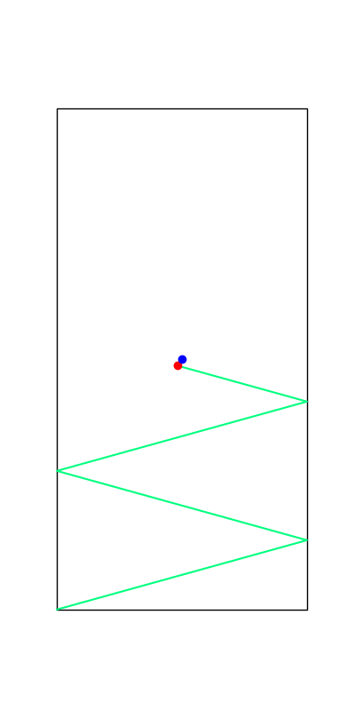
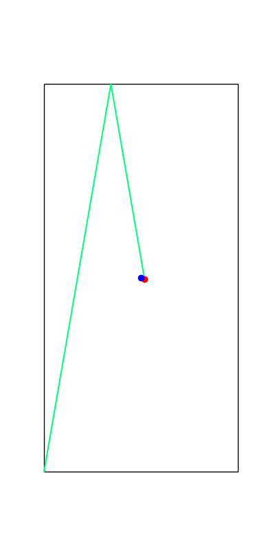
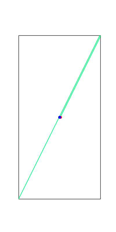
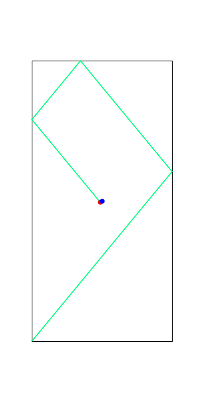
Results: Ball throwing on Wall
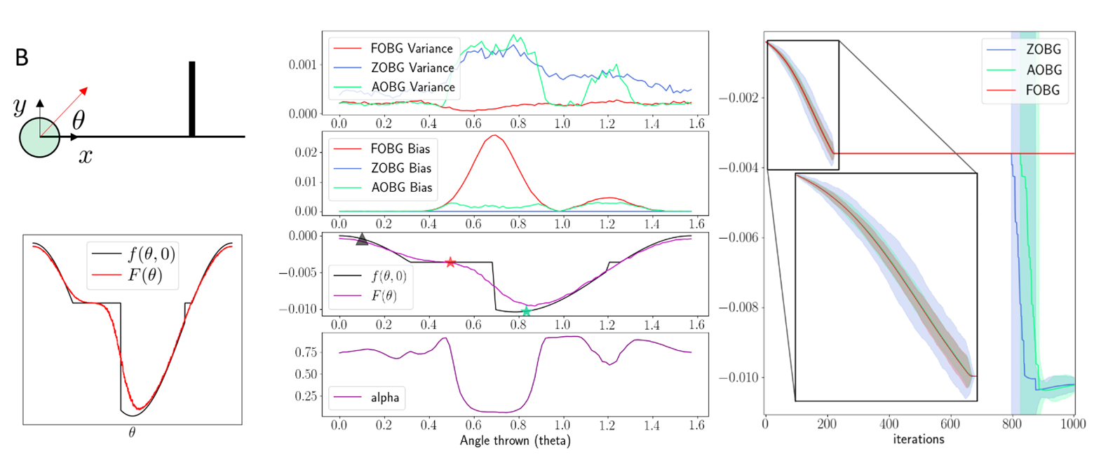
Key idea: Do not commit to zeroth or first uniformly,
but decide coordinate-wise which one to trust more.
Results: Policy Optimization
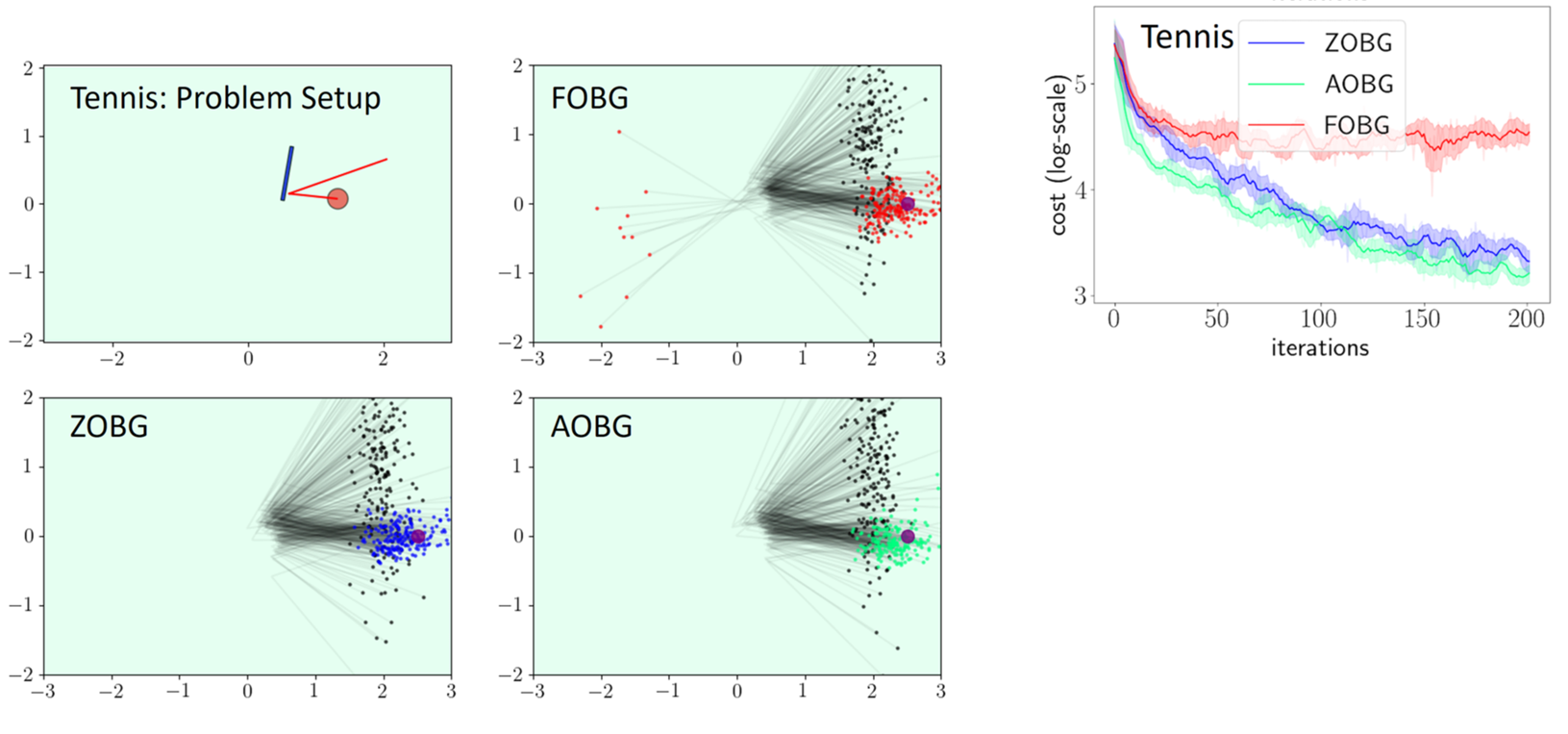
Able to capitalize on better convergence of first-order methods while being robust to their pitfalls.
Limitations of Smoothing
Contact is non-smooth. But Is it truly "discrete"?
The core thesis of this talk:
The local decisions of where to make contact are better modeled as continuous decisions with some smooth approximations.
My viewpoint so far:
Limitations of Smoothing
Contact is non-smooth. But Is it truly "discrete"?
The core thesis of this talk:
The local decisions of where to make contact are better modeled as continuous decisions with some smooth approximations.
My viewpoint so far:
The remaining "discrete decisions" come not from contact, but from discrete-level decisions during planning.
Smoothing CANNOT handle these high-level discrete decisions.
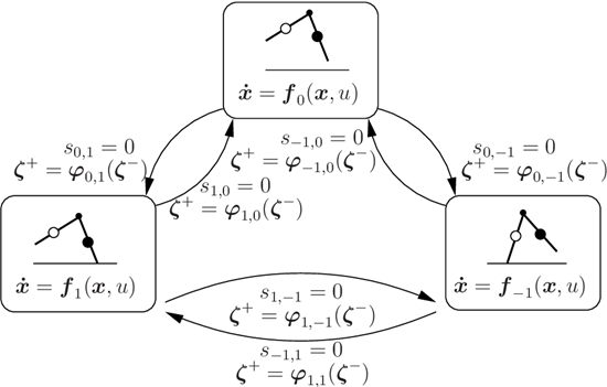
Limitations of Smoothing
These reveal true discrete "modes" of the decision making process.
Limitations of Smoothing
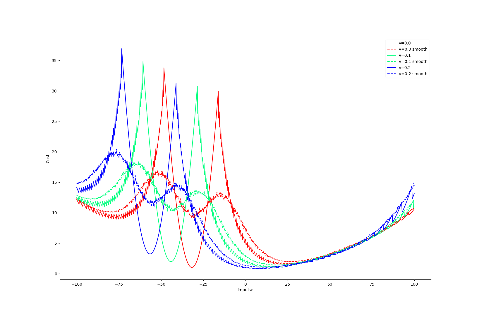
Apply negative impulse
to stand up.
Apply positive impulse to bounce on the wall.
Limitations of Smoothing
Can we smooth local contact decisions and efficiently search through high-level discrete decisions?
Our ideal solution
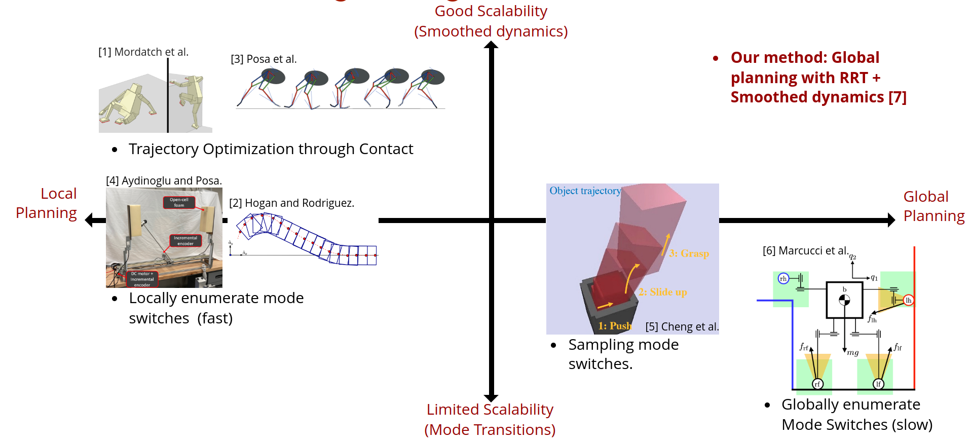
Global Search with Smoothing: Contact-Rich RRT
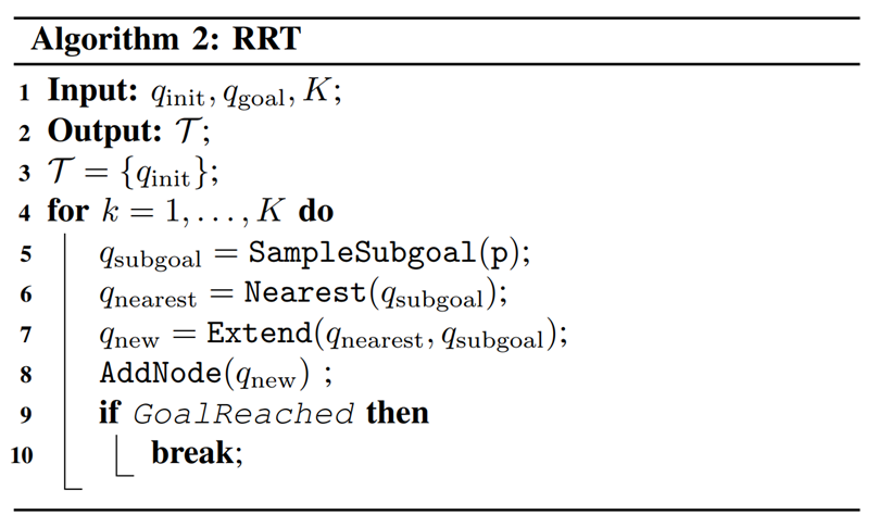
Motivating Contact-Rich RRT
Sampling-Based Motion Planning is a popular solution in robotics for complex non-convex motion planning
How do we define notions of nearest?
How do we extend (steer)?
- Nearest states in Euclidean space are not necessarily reachable according to system dynamics (Dubin's car)
- Typically, kinodynamic RRT solves trajopt
- Potentially a bit costly.
Reachability-Consistent Distance Metric
Reachability-based Mahalanobis Distance

How do we come up with a distance metric between q and qbar in a dynamically consistent manner?
Reachability-Consistent Distance Metric
Reachability-based Mahalanobis Distance
How do we come up with a distance metric between q and qbar in a dynamically consistent manner?
Consider a one-step input linearization of the system.
Then we could consider a "reachability ellipsoid" under this linearized dynamics,
Note: For quasidynamic formulations, ubar is a position command, which we set as the actuated part of qbar.
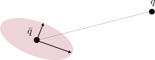
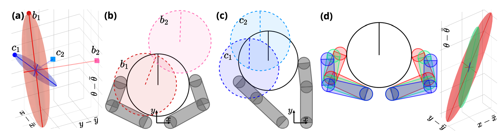
Reachability Ellipsoid
Reachability Ellipsoid
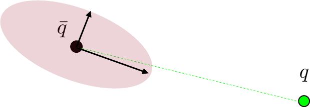
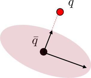
Intuitively, if B lengthens the direction towards q from a uniform ball, q is easier to reach.
On the other hand, if B decreases the direction towards q, q is hard to reach.
Mahalanobis Distance of an Ellipsoid
Reachability Ellipsoid
The B matrix induces a natural quadratic form for an ellipsoid,
Mahalanobis Distance using 1-Step Reachability
Note: if BBT is not invertible, we need to regularize to property define a quadratic distance metric numerically.
Smoothed Distance Metric
For Contact:
Don't use the exact linearization, but the smooth linearization.
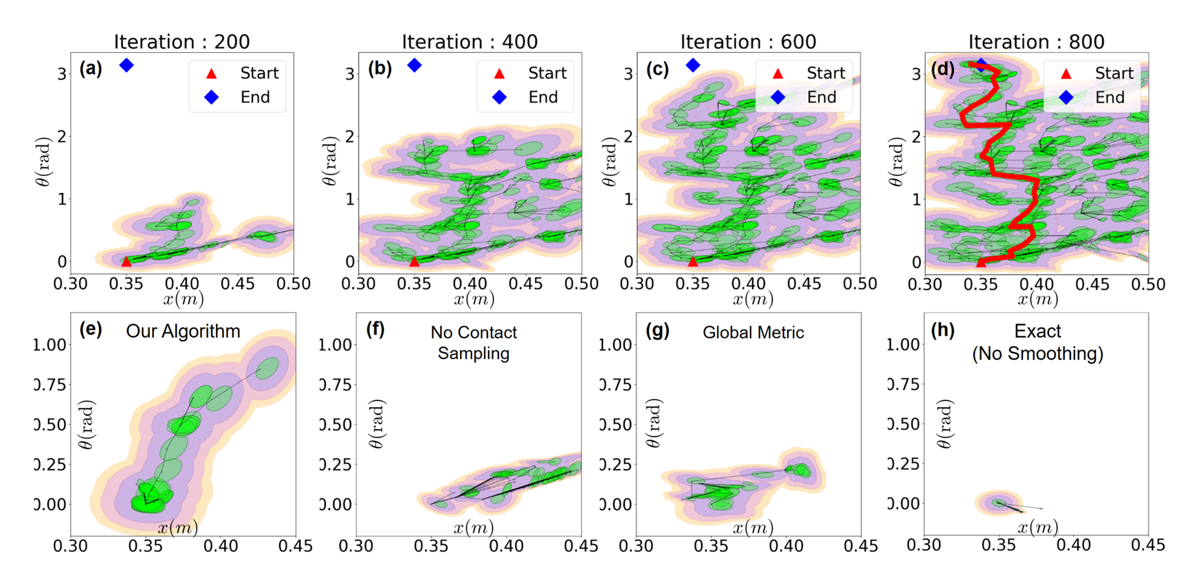
Global Search with Smoothing
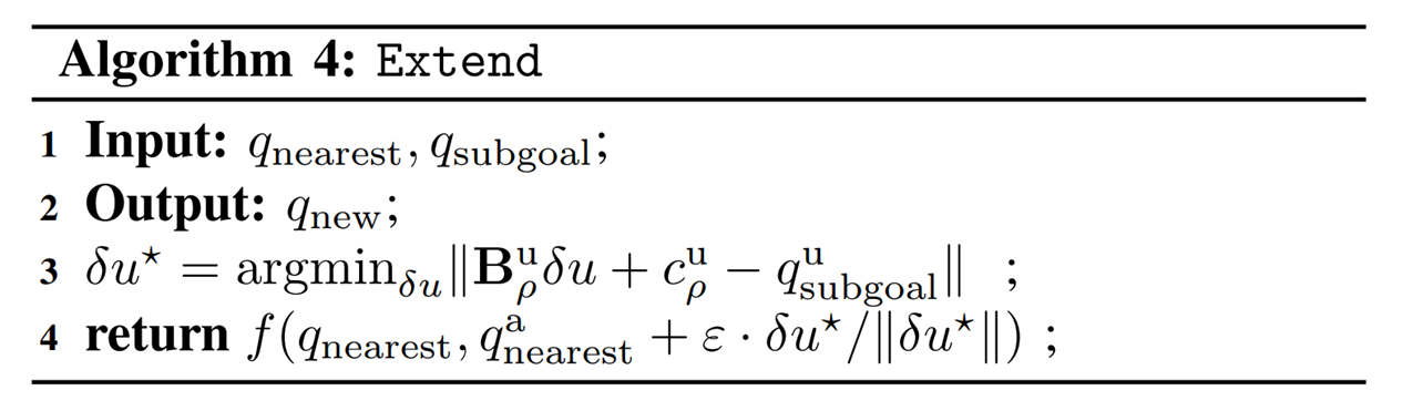
Dynamically consistent extension
Theoretically, it is possible to use long-horizon trajopt algorithms such as iLQR / DDP.
Here we simply do one-step trajopt and solve least-squares.
Importantly, the actuation matrix for least-squares is smoothed, but we rollout the actual dynamics with the found action.
Dynamically consistent extension
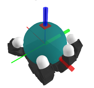
Contact Sampling
With some probability, we execute a regrasp (sample another valid contact configuration) in order to encourage further exploration.

Global Search with Smoothing
Before I go...


Will be hosting an IROS workshop on
Leveraging Models for Contact-Rich Manipulation.
https://sites.google.com/view/iros2023-contactrich/home
Excited to talk to more model-based folks who are interested in manipulation! (Or conversely, manipulation folks who still have an ounce of hope for models).
Thank you!
-
H.J. Terry Suh*, Tao Pang*, Russ Tedrake,
"Bundled Gradients through Contact via Randomized Smoothing",
RA-L 2022, Presented at ICRA 2022
-
H.J. Terry Suh, Max Simchowitz, Kaiqing Zhang, Russ Tedrake,
"Do Differentiable Simulators Give Better Policy Gradients?"
ICML 2022 Outstanding Paper Award,
2022 TC on Model-based Optimization for Robotics Best Paper Award
- Tao Pang*, H.J. Terry Suh*, Lujie Yang, Russ Tedrake,
"Global Planning for Contact-Rich Manipulation via Local Smoothing of Quasidynamic Contact Models",
To appear in Transactions of Robotics (T-RO)