A geometric interpretation of
(quantum) optimal transport
Thomas Borsoni\(^{1,2}\)
under the supervision of Virginie Ehrlacher\(^{1,2}\) & Geneviève Dusson\(^{3}\)
96\(^{\text{th}}\) annual GAMM meeting, Stuttgart
March 17\(^{\text{th}}\), 2026
\(^{1}\) CERMICS, ENPC, Champs-sur-Marne, France
\(^{2}\) MATHERIALS team, INRIA, France
\(^{3}\) Université Bourgogne-Franche-Comté, Besançon, France
Geometric interpretation
of classical and quantum optimal transport
Aim of the presentation
1. Classical and quantum optimal transport
Outline
2. Geometric interpretation of optimal transport
3. The folded Wasserstein distances
1. Classical and quantum optimal transport
Classical optimal transport

Principle
Given a cost \(c : E_1 \times E_2 \to \R\), construct a cost on \(\mathcal{P}(E_1) \times \mathcal{P}(E_2)\)
Given a distance \(d\) on \(E\), construct the Wasserstein-\(p\) distance on \(\mathcal{P}(E)\)
Formulations
1. Kantorovich primal: minimize a cost among couplings
2. Kantorovich dual: maximise a profit among potentials (prices)
3. Dynamic: minimize an energy along paths
Applications
Machine learning, image processing, economics, data sciences,...
- Mean-field limits of particle systems
- Geometry and analysis of spaces of probability measures
Aim
To compare probability measures: compute a cost or a distance
(+ interpolations)
Classical optimal transport
Aim
To compare probability measures: compute a cost or a distance
(+ interpolations)
Principle
Given a cost \(c : E_1 \times E_2 \to \R\), construct a cost on \(\mathcal{P}(E_1) \times \mathcal{P}(E_2)\)
Given a distance \(d\) on \(E\), construct the classical Wasserstein-\(p\) distance on \(\mathcal{P}(E)\)
Formulations
1. Kantorovich primal: minimize a cost among couplings
2. Kantorovich dual: maximise a profit among potentials (prices)
3. Dynamic: minimize an energy along paths
Applications
Machine learning, image processing, economics, data sciences,...
- Mean-field limits of classical particle systems
- Geometry and analysis of spaces of probability measures
Probability measures vs density matrices
Classical description:
System described at statistical level by a probability measure over a set \(E\)
Quantum description:
System described at statistical level by a density matrix over a Hilbert space \(\mathcal{H}\)
Probability measure \(\mu\)
Density matrix \(\rho\)
\(\cdot \; \; \mu\) is a measure on \(E\)
\(\cdot \; \; \mu \geq 0\)
\(\cdot \; \; \mu(E) = 1\)
\(\cdot \; \; \rho\) is a self-adjoint operator on \(\mathcal{H}\)
\(\cdot \; \; \rho \succeq 0\)
\(\cdot \; \; \mathrm{Trace}(\rho) = 1\)
"mixed" state
"pure" state
Dirac mass at \(\bm{\delta}_x\) for \(x \in E\)
\(x \in E\)
Projector onto \(\psi \in \mathcal{H}^*\)
\(\psi \in \mathcal{H}^* / \mathbb{C}^*\)
Quantum optimal transport
Aim
To compare density matrices: compute a cost or a distance
(+ interpolations)
Principle
Given a cost \(c\) on \((\mathcal{H}_1)^* / \mathbb{C}^* \times (\mathcal{H}_2)^* / \mathbb{C}^*\), construct a cost on \(\mathcal{D}(\mathcal{H}_1) \times \mathcal{D}(\mathcal{H}_2)\)
Given a distance \(d\) on \(\mathcal{H}^* / \mathbb{C}^*\), construct the quantum Wasserstein-\(p\) distance on \(\mathcal{D}(\mathcal{H})\)
Formulations
1. Kantorovich primal nonseparable: minimize a cost among all couplings
1'. Kantorovich primal separable: among couplings without entanglement
2. Kantorovich dual
3. Dynamic
Applications
Machine learning...
- Mean-field limits of quantum particle systems
- Geometry and analysis of spaces of density matrices
Golse-Mouhot-Paul, De Palma-Trevisan...
Tóth-Pitrik, Beatty-Stilck França...
Carlen-Maas
2. Geometric interpretation of optimal transport
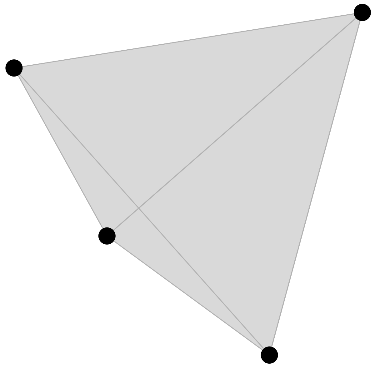
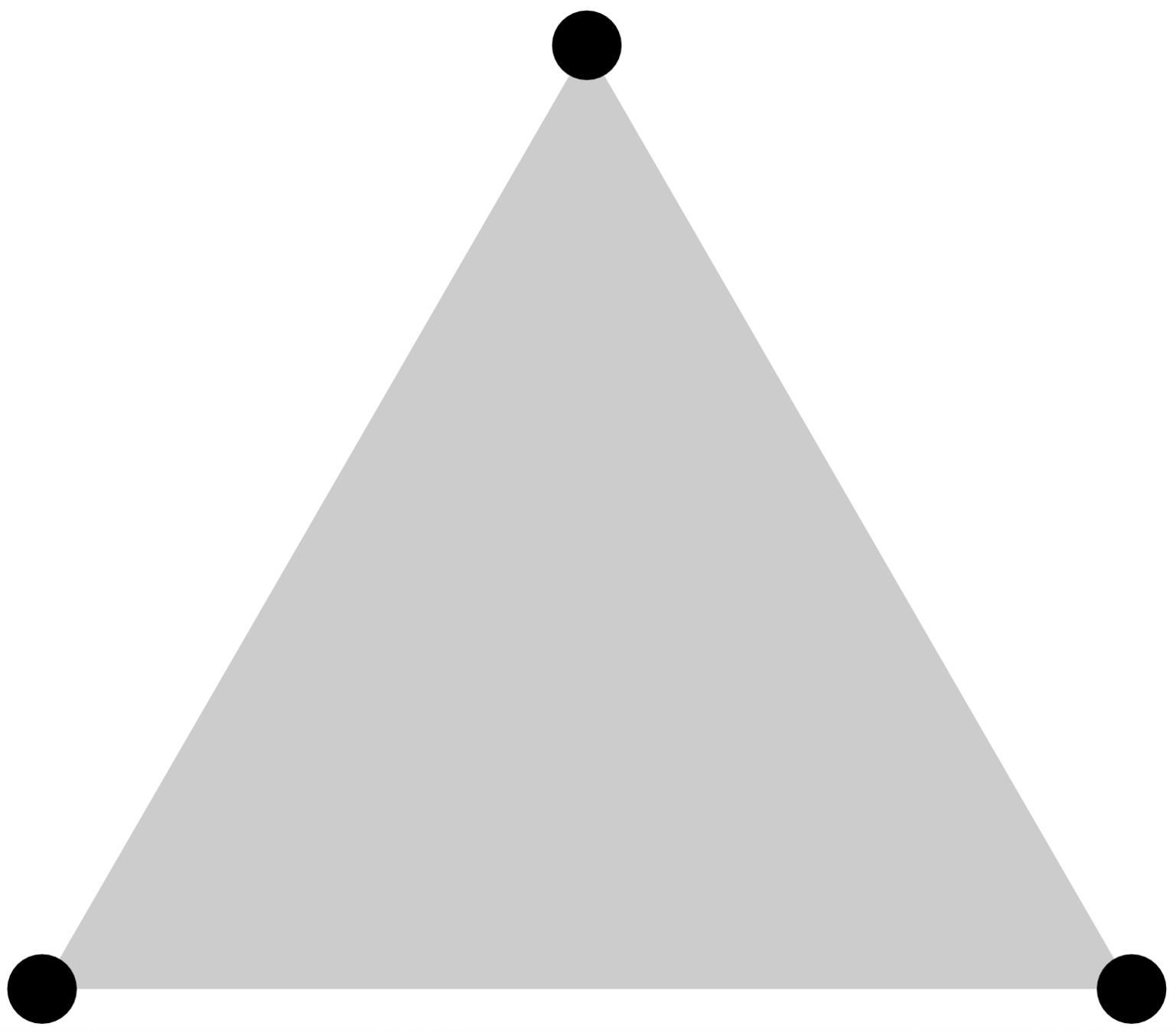
(good) illustration of a
set of probability measures
\(\bullet\) convex set
\(\bullet\) extreme boundary
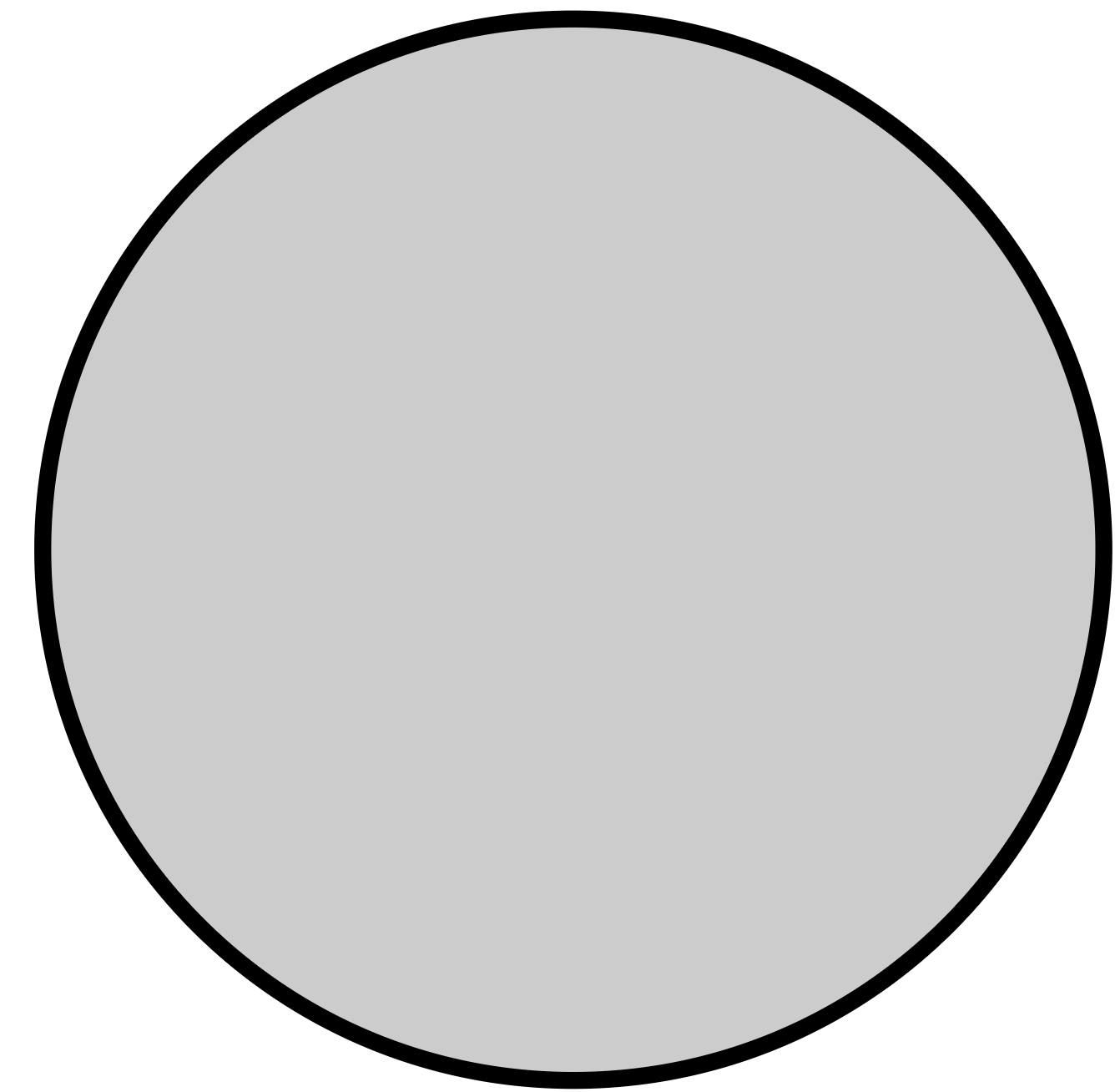
(not so good) illustration of a
set of density matrices
convex set
whose extreme boundary is \(\cong \mathcal{H}^* / \mathbb{C}^*\)
simplex
probability measure
convex combination
"mixed" states
"pure" states
- start with a distance \(d\) on \(E_0 \cong E\)
- construct a distance \(W_p\) on \(\mathcal{P}(E_0)\)
- \(\forall x,y \in E_0\), \(W_p\)\((\bm{\delta}_x, \bm{\delta}_y) = d(x,y)\)
Classical optimal transport extends a distance defined on the extreme boundary of a simplex to the whole simplex
Geometric interpretation of optimal transport
(case of a distance)
[Savaré-Sodini 22]
Classical
Quantum
Quantum optimal transport extends a distance defined on the extreme boundary of the convex \(\mathcal{D}(\mathcal{H})\) to the whole convex
- start with a distance \(d\) on \(\mathcal{H}^* / \mathbb{C}^*\)
- construct a distance \(D_p\) on \(\mathcal{D}(\mathcal{H})\)
- \({D_p}_{|\mathcal{H}^* / \mathbb{C}^*}\)\(= d\)
How to extend a distance \(d\) from \(E\) to \(C\)?
\(\bullet\) convex set \(C\)
\(\bullet\) extreme boundary \(E\)
classical optimal transport
quantum optimal transport
In general
How to extend a distance \(d\) from \(E\) to \(C\)?
\(\bullet\) convex set \(C\)
\(\bullet\) extreme boundary \(E\)
classical optimal transport
quantum optimal transport
In general
3. The folded Wasserstein distance
A possible answer:
Choquet theory
Representing every \(x \in C\) with convex combinations of points of \(E\)
- \(\mu_1 = \frac34 \bm{\delta}_{e_1} + \frac14 \bm{\delta}_{e'_1} \) represents \(x\)
(\(x\) is the barycenter associated with \(\mu_1\))
Representing every \(x \in C\) with probability measures \(\mu \in \mathcal{P}(E)\)
Choquet theory
Representing every \(x \in C\) with convex combinations of points of \(E\)
Representing every \(x \in C\) with probability measures \(\mu \in \mathcal{P}(E)\)
- \(\mu_1 = \frac34 \bm{\delta}_{e_1} + \frac14 \bm{\delta}_{e'_1} \) represents \(x\)
- \(\mu_2 = \frac12 \bm{\delta}_{e_2} + \frac12 \bm{\delta}_{e'_2} \) represents \(x\)
(\(x\) is the barycenter associated with \(\mu_1\))
(\(x\) is the barycenter associated with \(\mu_2\))
Choquet theory
Representing every \(x \in C\) with convex combinations of points of \(E\)
Representing every \(x \in C\) with probability measures \(\mu \in \mathcal{P}(E)\)
- \(\mu_3 = \frac14 \bm{\delta}_{e_3} + \frac14 \bm{\delta}_{e'_3} + \frac12 \bm{\delta}_{e''_3} \) represents \(x\)
- \(\mu_1 = \frac34 \bm{\delta}_{e_1} + \frac14 \bm{\delta}_{e'_1} \) represents \(x\)
- \(\mu_2 = \frac12 \bm{\delta}_{e_2} + \frac12 \bm{\delta}_{e'_2} \) represents \(x\)
(\(x\) is the barycenter associated with \(\mu_1\))
(\(x\) is the barycenter associated with \(\mu_2\))
(\(x\) is the barycenter associated with \(\mu_3\))
Choquet theory
Representing every \(x \in C\) with convex combinations of points of \(E\)
Representing every \(x \in C\) with probability measures \(\mu \in \mathcal{P}(E)\)
- \(\mu_1 = \frac34 \bm{\delta}_{e_1} + \frac14 \bm{\delta}_{e'_1} \) represents \(x\)
- \(\mu_2 = \frac12 \bm{\delta}_{e_2} + \frac12 \bm{\delta}_{e'_2} \) represents \(x\)
- \(\mu_3 = \frac14 \bm{\delta}_{e_3} + \frac14 \bm{\delta}_{e'_3} + \frac12 \bm{\delta}_{e''_3} \) represents \(x\)
many \(\mu \in \mathcal{P}(E)\) represent \(x\) !
(\(x\) is the barycenter associated with many \(\mu \in \mathcal{P}(E)\))
- \(\mu_1 = \frac34 \bm{\delta}_{e_1} + \frac14 \bm{\delta}_{e'_1} \) represents \(x\)
- \(\mu_2 = \frac12 \bm{\delta}_{e_2} + \frac12 \bm{\delta}_{e'_2} \) represents \(x\)
- \(\nu = \frac23 \bm{\delta}_{g} + \frac13 \bm{\delta}_{g'}\) represents \(y \neq x\)
\(\mu_1\) \(\sim \) \(\mu_2\)
\(\mu_1\), \(\mu_2\) \(\nsim \) \(\nu\)
then
but
- Let \(\sim\) be the equivalence relation on \(\mathcal{P}(E)\):
\(\mu\) and \(\nu\) represent the same \(x \in C\),
Choquet theory
Choquet-Bishop-DeLeeuw Theorem:
If \(C\) is convex and compact *, then
* and subset to a locally convex Hausdorff space
(\(x\) is the barycenter associated with at least one \(\mu \in \mathcal{P}(E)\))
Since
\(\mu\) and \(\nu\) represent the same \(x \in C\),
Choquet-Bishop-DeLeeuw
there exists at least one \(\mu \in \mathcal{P}(E)\) which represents \(x\)
Representing every \(x \in C\) with probability measures \(\mu \in \mathcal{P}(E)\)
Choquet theory
unfold
extend
fold back
with classical optimal transport
Folded Wasserstein distance on \(C\): \(D_p := W_p / \sim\)
(Choquet)
How to extend \(d\) from \(E\) to \(C\)?
?
represent
quotient
Folded Wasserstein
[B. 25]
The quotient (pseudo-)distance
*pseudo-distance: would be a distance if it separated points
a priori, fails the triangle inequality!
- Candidate quotient distance:
- The actual quotient pseudo*-distance:
?
on
The folded Wasserstein metric space
Theorem
- \(C\) compact convex subset of \((X,\|\cdot\|)\) Banach
- \((E,d)\) compact Polish and \(d\) continuous w.r.t. \(\|\cdot\|\)
- For all \(x,y \in E\), \(d(x,y) \geqslant \|x-y\| \)
Assume:
Then:
- \(D_p\) is a distance on \(C\), and if* \(\mathrm{Ri}(C) \neq \emptyset\), is continuous w.r.t. \(\|\cdot\|\)
- For all \(x,y \in C\), \(D_p(x,y) \geqslant \|x-y\|\)
- \(D_p\) sub-extends \(d\), and if \(d = \|\cdot - \cdot\|\), \(D_p\) extends \(d\)
A possible answer to: how to extend \(d\) from \(E\) to \(C\)?
*\(\mathrm{Ri}(C)\) is the relative interior of \(C\). In finite dimension, \(C \neq \emptyset \implies \mathrm{Ri}(C) \neq \emptyset\).
\(\forall x,y \in E\), \(D_p(x,y) \leqslant d(x,y) \) \(\forall x,y \in E\), \(D_p(x,y) = d(x,y) \)
- If \((E,d)\) is geodesic and \(p>1\), then \((C,D_p)\) is geodesic
[B. 25]
- Classical optimal transport extends a cost from the extreme boundary of a simplex to the whole simplex
- Quantum Kantorovich OT without entanglement is folded OT with the convex \(\mathcal{D}(\mathcal{H})\)
- Folded OT is constructed from classical OT
Conclusion
- Folded optimal transport extends a cost from the extreme boundary of a (compact) convex to the whole convex
Perspective
- Quantum Kantorovich OT with entanglement using noncommutative convexity
a generalization of classical OT