CS5001 / CS5003:
Intensive Foundations of Computer Science
Lecture 10: Searching and Sorting

Today's topics:
- Searching
- Linear Search
- Binary Search
- Sorting
- Selection Sort
- Insertion Sort
- Merge Sort
- Quicksort
Lecture 10: Searching and Sorting
- Searching is when we find something in a data structure. We frequently search for strings in things like web pages, PDFs, documents, etc., but we can also search through other data structures, like lists, dictionaries, etc.
- Depending on how our data is organized, we can search in different ways. For unorganized data, we usually have to do a linear search, which is the first type of search we will discuss.
- If our data is organized in some way, we can do more efficient searches. If our data is in a strict order, we can perform a binary search, which is the second type of search we will look at.
Lecture 10: Searching
- The most straightforward type of search is the linear search.
- We traverse the data structure (e.g., a string's characters, or a list) until we find the result. How would we do a linear search on a list, like this? Let's say we are searching for 15.
Lecture 10: Linear Searching
lst = [12, 4, 9, 18, 53, 82, 15, 99, 98, 14, 11]- The most straightforward type of search is the linear search.
- We traverse the data structure (e.g., a string's characters, or a list) until we find the result. How would we do a linear search on a list, like this? Let's say we are searching for 15.
Lecture 10: Linear Searching
lst = [12, 4, 9, 18, 53, 82, 15, 99, 98, 14, 11]def linear_search(lst, value_to_find):
"""
Perform a linear search to find a value in the list
:param lst: a list
:param value_to_find: the value we want to find
:return: the index of the found element, or -1 if the element does not
exist in the list
>>> linear_search([12, 4, 9, 18, 53, 82, 15, 99, 98, 14, 11], 15)
6
>>> linear_search([12, 4, 9, 18, 53, 82, 15, 99, 98, 14, 11], 42)
-1
"""
for i, value in enumerate(lst):
if value == value_to_find:
return i
return -1- What if we want to find a substring inside a string? Python, of course, has a string search algorithm built-in (
s.find()), but let's think about how we might do this.
Lecture 10: Linear Searching
s = "The cat in the hat"
find_str(s, "cat")- What if we want to find a substring inside a string? Python, of course, has a string search algorithm built-in (
s.find()), but let's think about how we might do this.
Lecture 10: Linear Searching
s = "The cat in the hat"
find_str(s, "cat")
def find_str(s, str_to_find):
"""
Returns the index of the first occurrence of str_to_find in s, and -1 if
the string is not contained in s
:param s: a string
:param str_to_find: the string to search for
:return: the index of the first occurrence of str_to_find in s,
-1 if not found
>>> find_str("the cat in the hat", "cat")
4
>>> find_str("aaaaab", "aab")
3
"""
for i in range(len(s) - len(str_to_find) + 1):
found = True
for c, c_to_find in zip(s[i:], str_to_find):
if c != c_to_find:
found = False
break
if found:
return i- Linear searching is slow! Why?
- Instead of performing a linear search, we can drastically speed up our searches if we first order what we are searching (this is sorting, which we will cover next!)
- We have discussed binary searches in class before -- the best example of when to use a binary search is the classic "find my number" game where someone thinks of a number between 1 and 100, and the player tries to guess. If the player guesses incorrectly, the number-chooser tells the player if their guess was too low or too high, and then the player guesses again.
- What is the best strategy for the guess-my-number game?
Lecture 10: Binary Searching
- Linear searching is slow! Why?
- Instead of performing a linear search, we can drastically speed up our searches if we first order what we are searching (this is sorting, which we will cover next!)
- We have discussed binary searches in class before -- the best example of when to use a binary search is the classic "find my number" game where someone thinks of a number between 1 and 100, and the player tries to guess. If the player guesses incorrectly, the number-chooser tells the player if their guess was too low or too high, and then the player guesses again.
- What is the best strategy for the guess-my-number game?
- First, guess the number in the middle.
- If the guess is too low, guess the number between the middle and the top, or the middle and the bottom.
- Keep narrowing by finding the "next middle" until you win
Lecture 10: Binary Searching
- What is the best strategy for the guess-my-number game?
- First, guess the number in the middle.
- If the guess is too low, guess the number between the middle and the top, or the middle and the bottom.
- Keep narrowing by finding the "next middle" until you win
- Why is this fast?
- It divides the amount of numbers left to search by 2 each time. If you start with 100 numbers, you have to guess at most 7 times. E.g.:
- Number picked: 1
- Guess: 50, then 25, then 12, then 6, then 3, then 1
- Number picked: 100
- Guess: 50, then 75, then 88, then 93, then 96, then 98, then 100.
Lecture 10: Binary Searching
- In Python, we would write the algorithm like this:
Lecture 10: Binary Searching
def binary_search(sorted_list, value_to_find):
    """
    Performs a binary search on sorted_list for value_to_find
    :param sorted_list: a sorted list, smallest to largest
    :param value_to_find: the value we are looking for
    :return: the index of value_to_find, or -1 if not found
    """
    low = 0  # the low index
    high = len(sorted_list) - 1  # the high index
    while low <= high:
        mid = (low + high) // 2  # the middle value
        if sorted_list[mid] < value_to_find:
            low = mid + 1
        elif sorted_list[mid] > value_to_find:
            high = mid - 1
        else:  # found!
            return mid
return -1- Be sure you understand how this algorithm works!
- Can we calculate the maximum number of guesses a binary search will take? Sure!
- Each guess splits the amount of the list we have to search by a factor of 2. Let's see what this means for 16 elements, if we guess incorrectly until we reach one element. The number of elements left will drop by half each time:
- 16 -> 8 -> 4 ->2 ->1
- This was four total divisions (16/2 = 8, 8/2=4, 4/2=2, 2/2 = 1), so we have:
Lecture 10: Binary Searching
- In general, this becomes:
where n is the number of elements, and k is the number of times we have to divide.
Lecture 10: Binary Searching
- We can simplify:
- We can take the log2 of both sides to get:
- And we get (after swapping sides):
- Therefore, the maximum number of steps, k, for a binary search is log2(n).
- For n =100, log2(100) = 6.64, or a maximum of 7 steps.
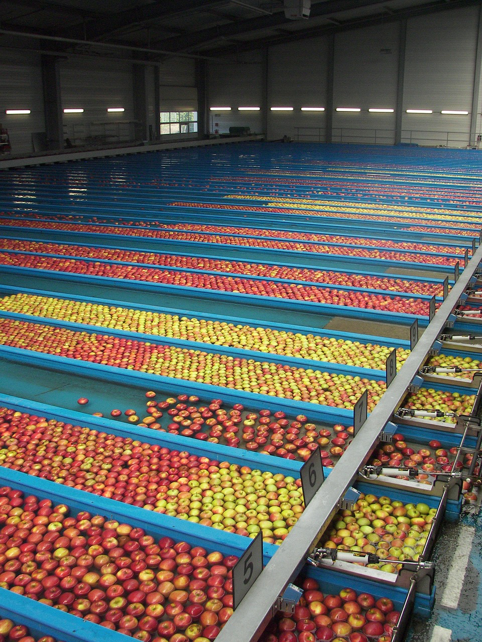
Lecture 10: Sorting
- In general, sorting consists of putting elements into a particular order, most often the order is numerical or lexicographical (i.e., alphabetic).
-
In order for a list to be sorted, it must:
- be in nondecreasing order (each element must be no smaller than the previous element)
- be a permutation of the input

Lecture 10: Sorting
- Sorting is a well-researched subject, although new algorithms do arise (see Timsort, from 2002)
Fundamentally, comparison can only be so good -- we will see some fast sorts and some not-so-fast sorts.

- Although we haven't studied it yet (it is coming up!), the best comparison sorts can only sort in the average case as fast as "n log n" -- that is, take the number of elements, n, and multiply by log n, and that is the best number of comparisons we have to do to sort the elements.
Lecture 10: Sorting
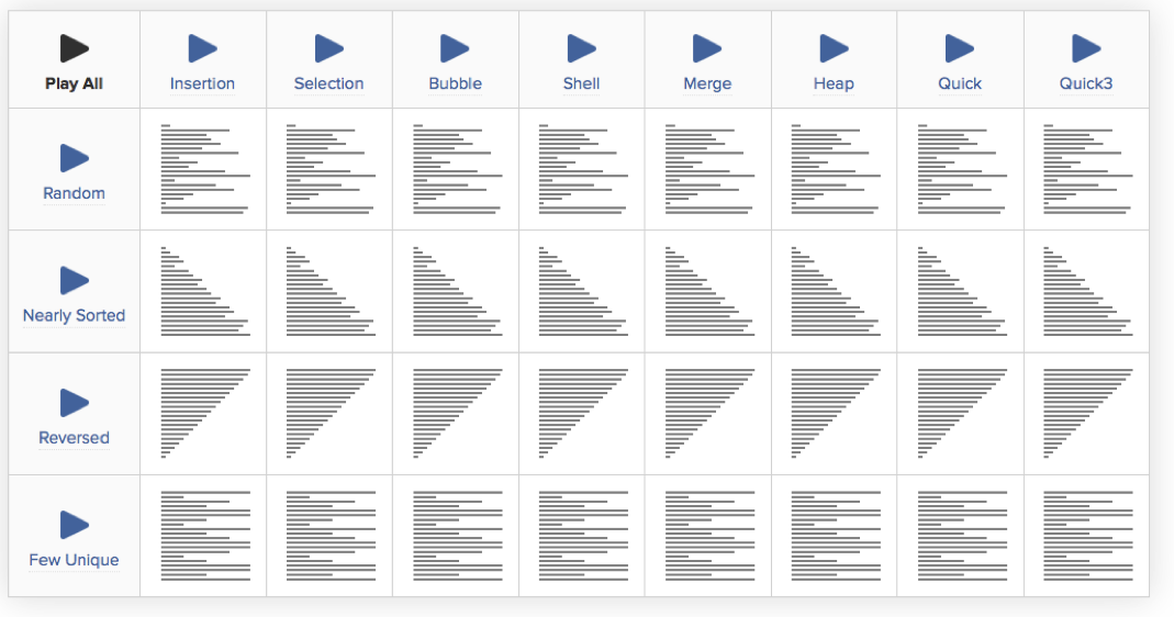
- There are some phenomenal online sorting demonstrations: see the “Sorting Algorithm Animations” website:
- http://www.sorting-algorithms.com, or the animation site at: http://www.cs.usfca.edu/~galles/visualization/ComparisonSort.html or the cool “15 sorts in 6 minutes” video on YouTube: https://www.youtube.com/watch?v=kPRA0W1kECg
Lecture 10: Sorting
- There are many, many different ways to sort elements in a list. We will look at the following
Insertion Sort
Selection Sort
Merge Sort
Quicksort
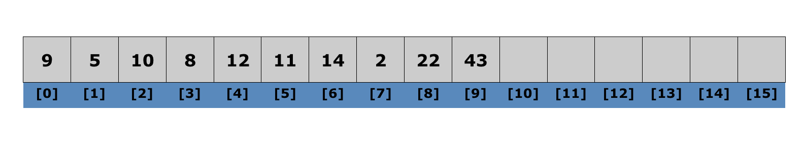
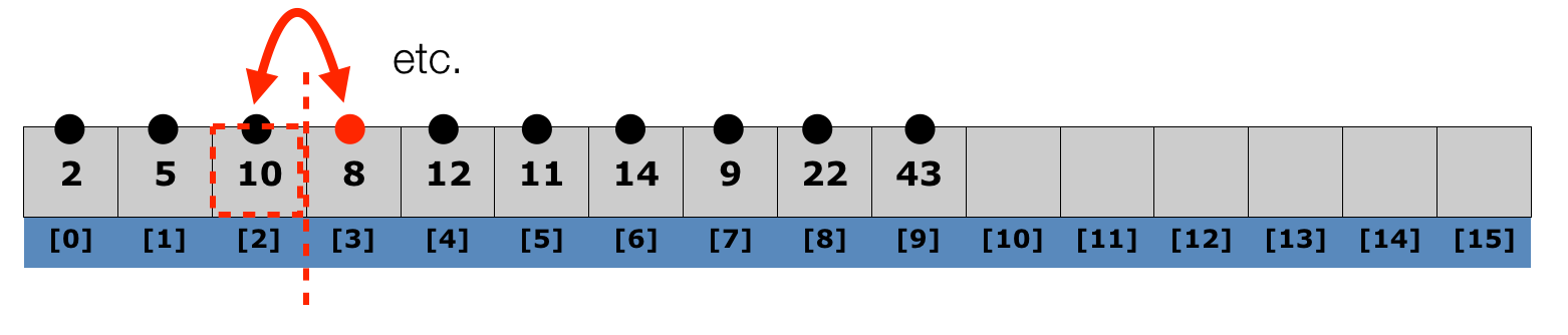
Lecture 10: Insertion Sort
-
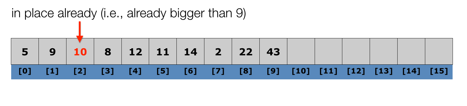
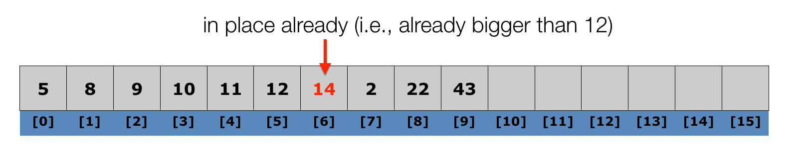
Insertion sort: orders a list of values by repetitively inserting a particular value into a sorted subset of the list
-
More specifically:
– consider the first item to be a sorted sublist of length 1
– insert second item into sorted sublist, shifting first item if needed
– insert third item into sorted sublist, shifting items 1-2 as needed
– ...
– repeat until all values have been inserted into their proper positions
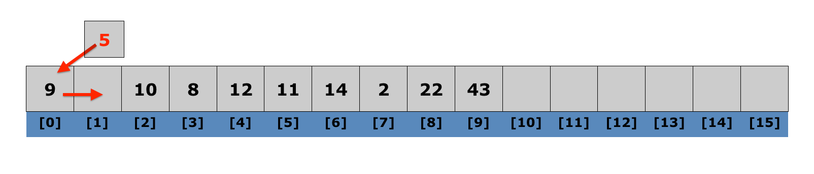
Lecture 10: Insertion Sort
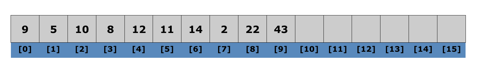
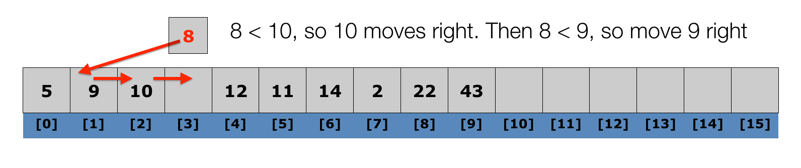
Algorithm:
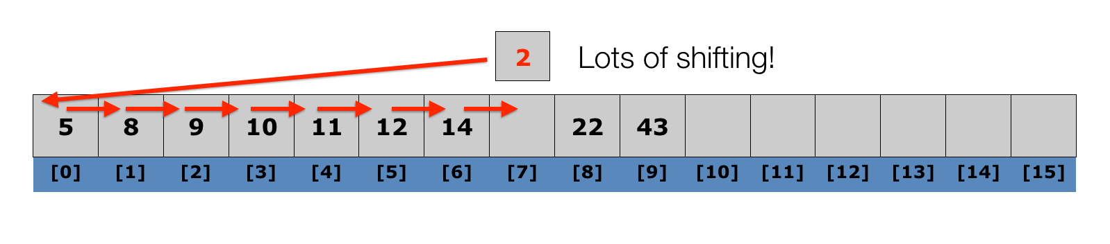
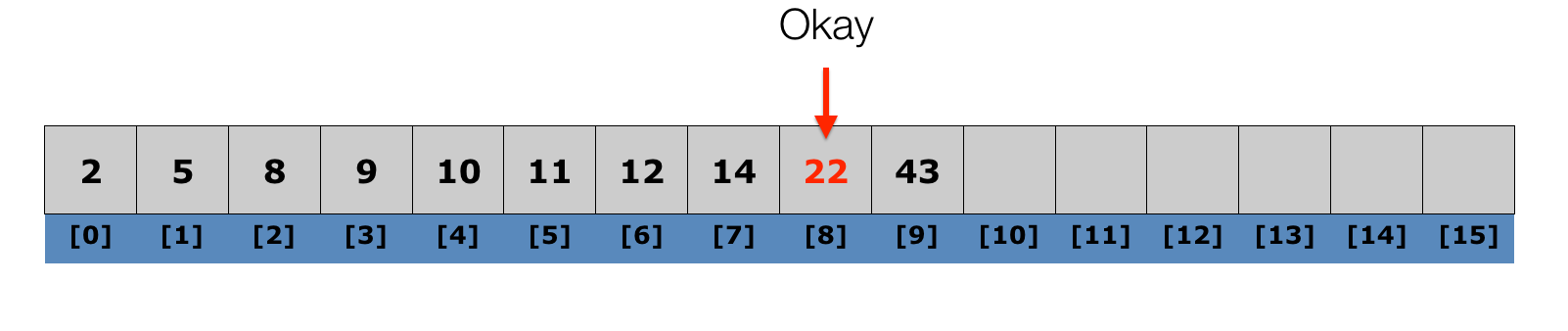
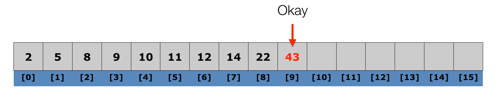
- iterate through the list (starting with the second element)
- at each element, shuffle the neighbors below that element up until the proper place is found for the element, and place it there.
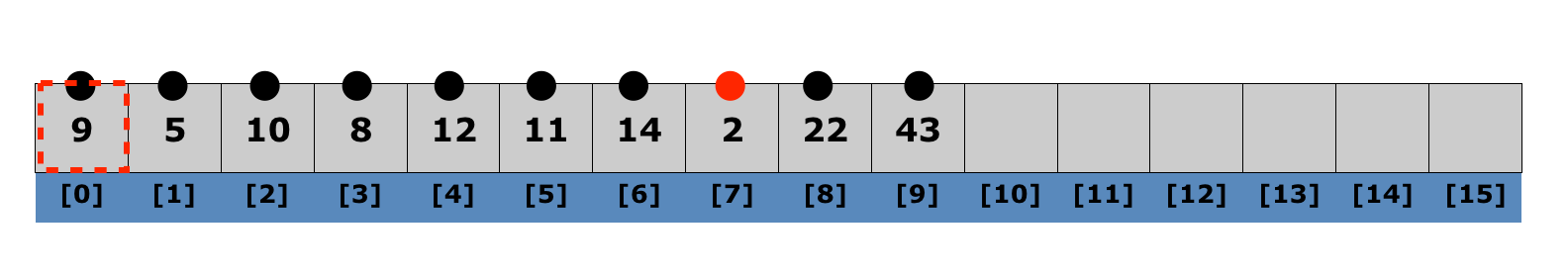
Lecture 10: Insertion Sort
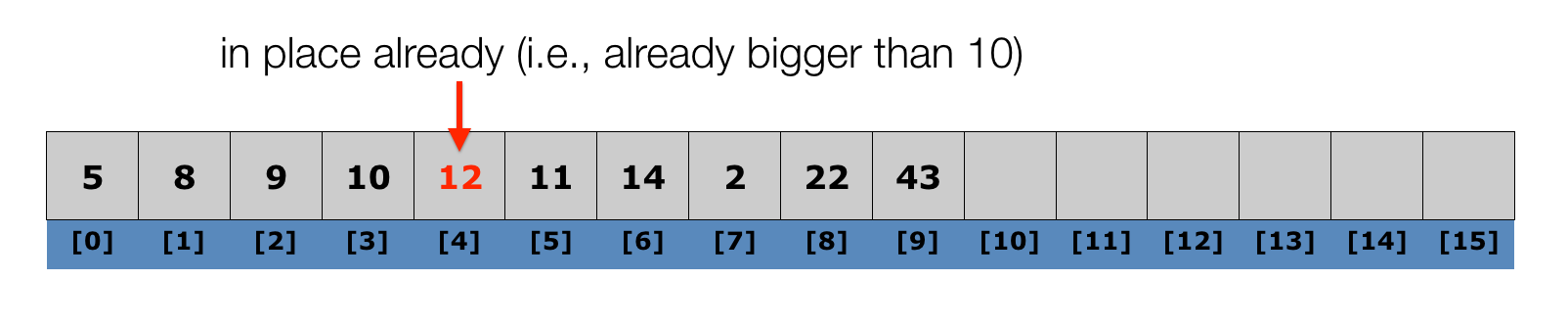
Algorithm:
- iterate through the list (starting with the second element)
- at each element, shuffle the neighbors below that element up until the proper place is found for the element, and place it there.
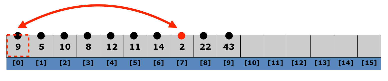
Lecture 10: Insertion Sort
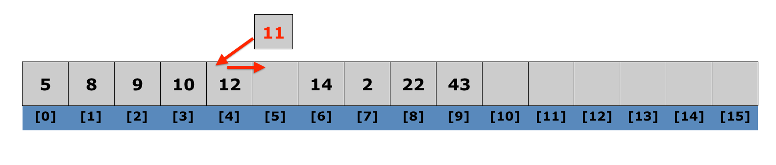
Algorithm:
- iterate through the list (starting with the second element)
- at each element, shuffle the neighbors below that element up until the proper place is found for the element, and place it there.
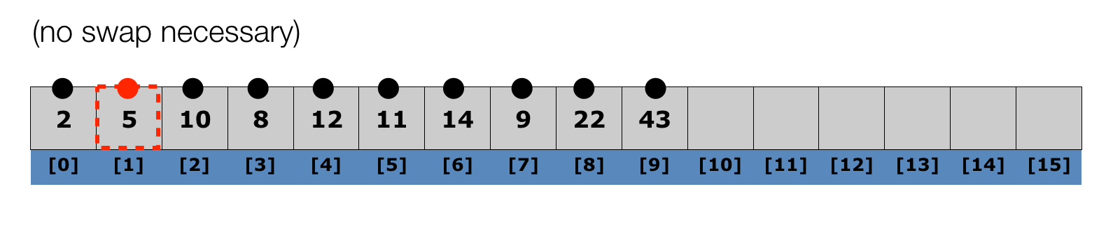
Lecture 10: Insertion Sort
Algorithm:
- iterate through the list (starting with the second element)
- at each element, shuffle the neighbors below that element up until the proper place is found for the element, and place it there.
Lecture 10: Insertion Sort
Algorithm:
- iterate through the list (starting with the second element)
- at each element, shuffle the neighbors below that element up until the proper place is found for the element, and place it there.
Lecture 10: Insertion Sort
Algorithm:
- iterate through the list (starting with the second element)
- at each element, shuffle the neighbors below that element up until the proper place is found for the element, and place it there.
Lecture 10: Insertion Sort
Algorithm:
- iterate through the list (starting with the second element)
- at each element, shuffle the neighbors below that element up until the proper place is found for the element, and place it there.
Lecture 10: Insertion Sort
Algorithm:
- iterate through the list (starting with the second element)
- at each element, shuffle the neighbors below that element up until the proper place is found for the element, and place it there.
Lecture 10: Insertion Sort
Algorithm:
- iterate through the list (starting with the second element)
- at each element, shuffle the neighbors below that element up until the proper place is found for the element, and place it there.
Lecture 10: Insertion Sort
Best case? The list is already sorted -- nothing to do!
Worst case? The list is completely reversed -- we have to shift the entire list each time!
The best case is said to be "linear" in that we only have to go through the list once (we have to look at n elements).
The worst case is called n2, because we have to look through (and move) all the remaining elements each time.
Lecture 10: Insertion Sort
Insertion sort code:
def insertion_sort(lst):
    for i in range(1,len(lst)):
        temp = lst[i]
        j = i
        while j >= 1 and lst[j - 1] > temp:
            lst[j] = lst[j - 1]
            j -= 1
        lst[j] = temp
Insertion sort is an easy sort to code, and it is decently fast for small lists.
Lecture 10: Selection Sort
-
Selection Sort is another in-place sort that has a simple algorithm:
- Find the smallest item in the list, and exchange it with the left-most unsorted element.
- Repeat the process from the first unsorted element.
- See animation at: http://www.cs.usfca.edu/~galles/visualization/ComparisonSort.html
Lecture 10: Selection Sort
-
Algorithm
- Find the smallest item in the list, and exchange it with the left-most unsorted element.
- Repeat the process from the first unsorted element.
- Selection sort is particularly slow, because it needs to go through the entire list each time to find the smallest item.
Lecture 10: Selection Sort
- Selection sort is always an n2 algorithm, because you don't get the benefit if the list is already sorted -- you always have to find the next smallest element.
- What might selection sort be good for?
- If you want to find the "top X" elements, you can do so relatively fast (at least as fast as any other algorithm, anyway)
Lecture 10: Selection Sort
- Selection sort is also easy to write, but unless you want to find the top X, it is worth it to simply write insertion sort, instead.
def selection_sort(lst):
    for i in range(len(lst)):
        min_index = i
        for j in range(i + 1, len(lst)):
            if lst[j] < lst[min_index]:
                min_index = j
lst[i], lst[min_index] = lst[min_index], list[i]- Selection sort code:
Lecture 10: Merge Sort
- So far, we have seen sorts that have bad worst-case performance (and in the case of selection sort, always have bad performance).
- Now, we are going to look at a sort called merge sort that has good performance, always.
- Merge sort uses the same basic idea as binary search: split the problem into halves as much as you can, leading to logarithmic behavior. Merge sort is called a divide-and-conquer algorithm because of this splitting.
- Merge sort can be coded recursively, so we will look at that.
- The basic idea of merge sort is to sort already sorted lists. For example:
- lst1 = [3, 5, 11]
- lst2 = [1, 8, 10]
- merge(lst1, lst2) produces [1, 3, 5, 8, 10, 11]
Lecture 10: Merge Sort
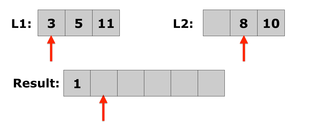
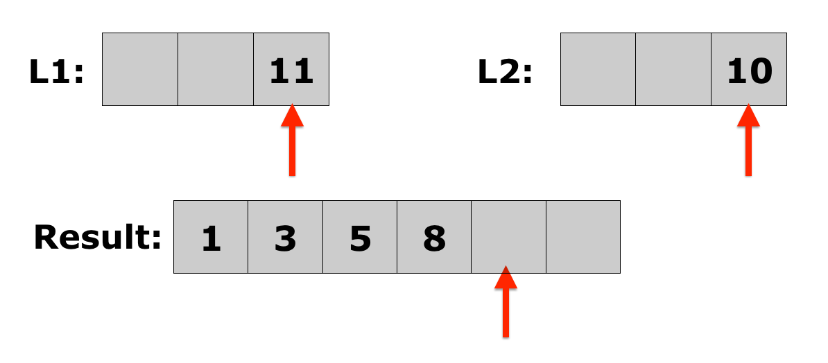
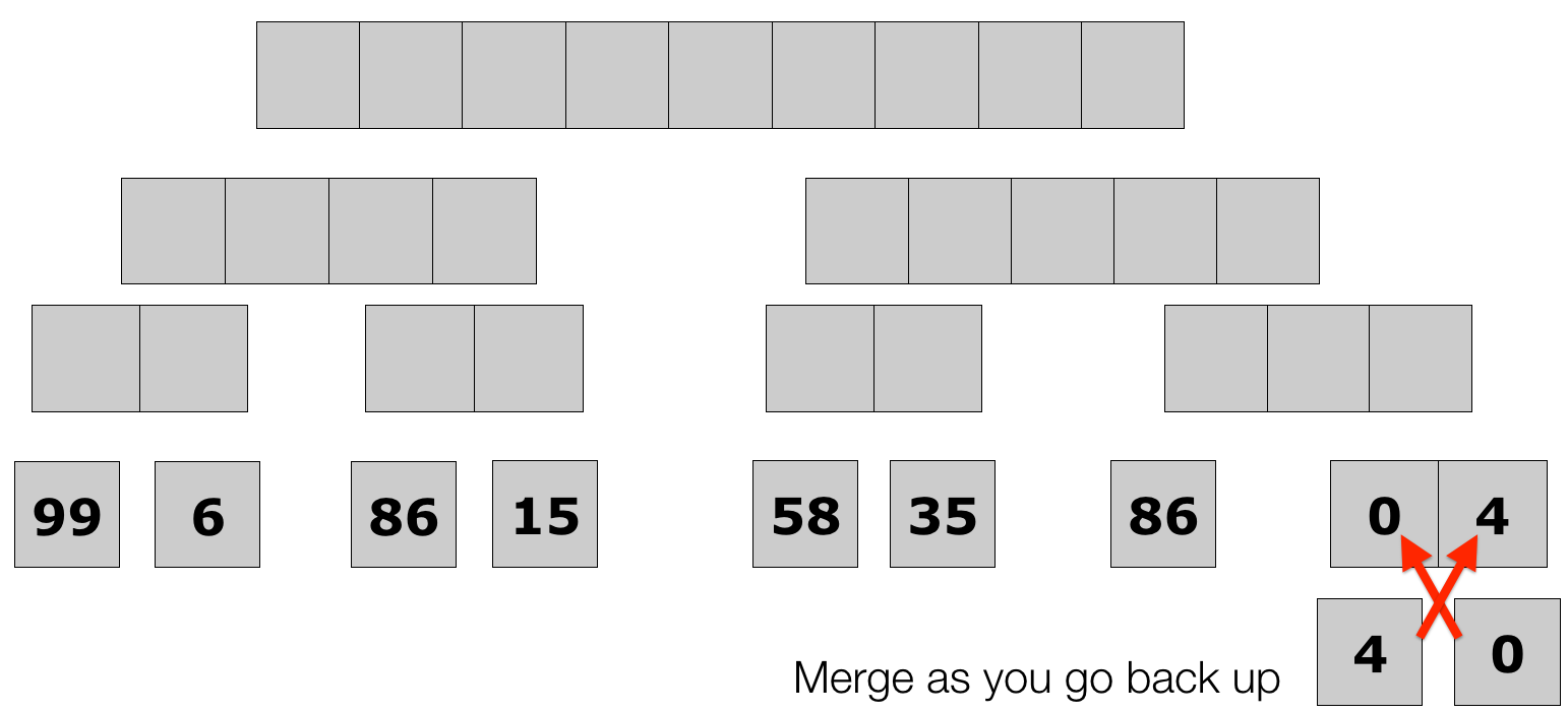
- Merging two sorted lists is easy:
- Choose the first element in each list.
- Compare the two elements, and append the smallest one to the new list.
- Choose the next smallest element from the list that just lost an element, and keep the element that was not appended. Repeat from step 2 until there is only one list left with elements, at which point you go to step 4.
- Append the remaining elements onto the new list.

Lecture 10: Merge Sort
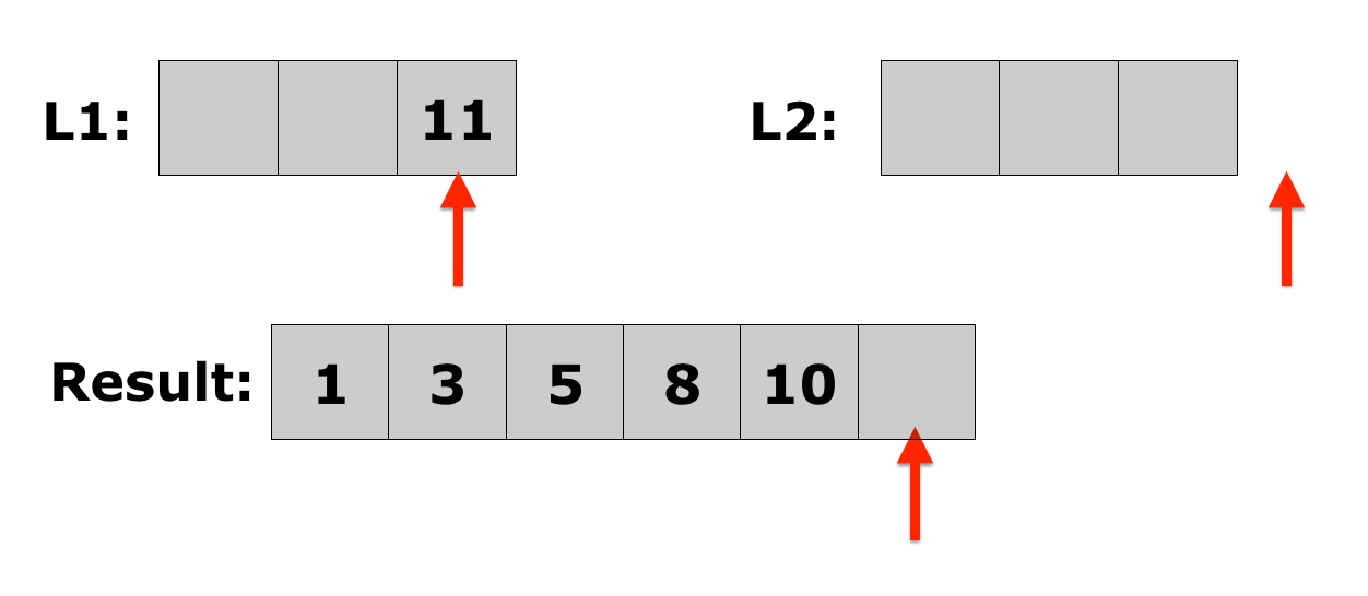
- Merging two sorted lists is easy:
- Choose the first element in each list.
- Compare the two elements, and append the smallest one to the new list.
- Choose the next smallest element from the list that just lost an element, and keep the element that was not appended. Repeat from step 2 until there is only one list left with elements, at which point you go to step 4.
- Append the remaining elements onto the new list.
Lecture 10: Merge Sort
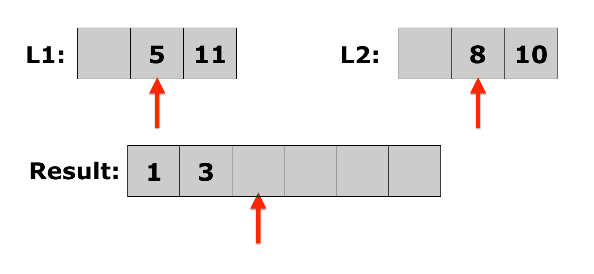
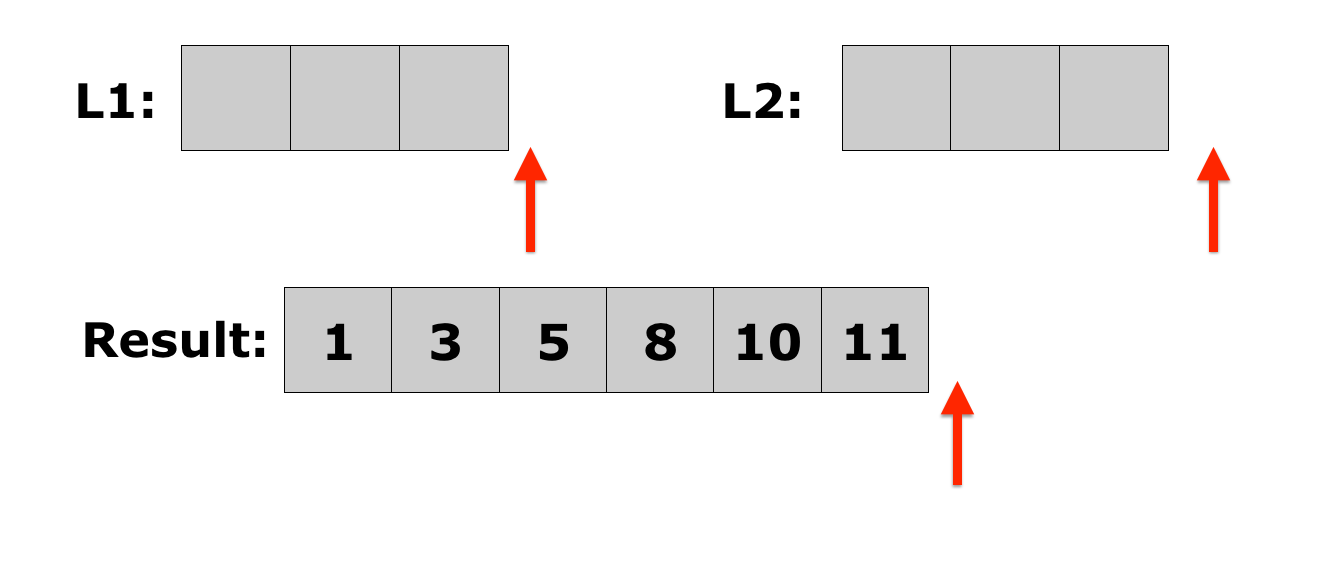
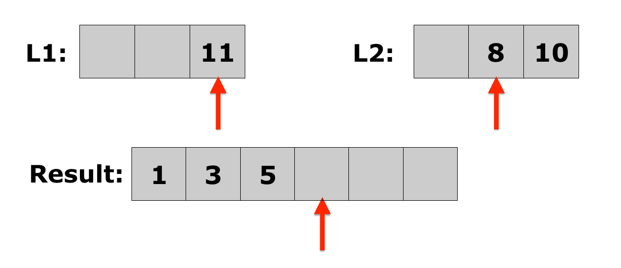
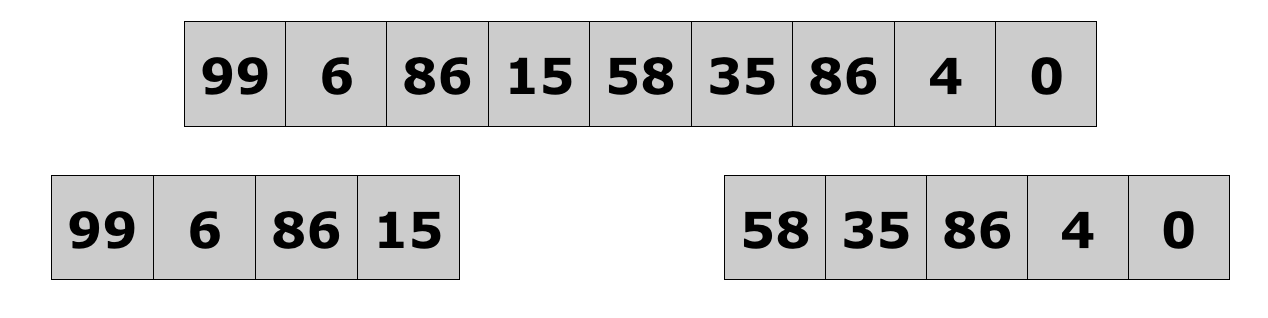
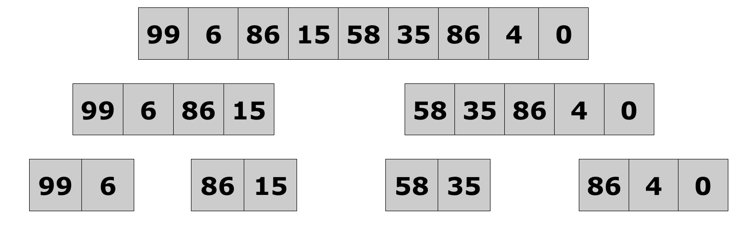
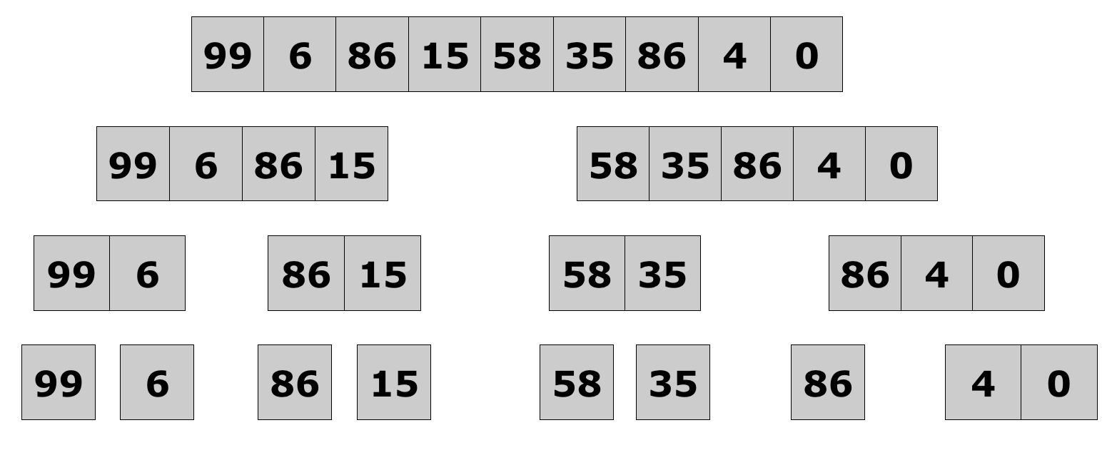
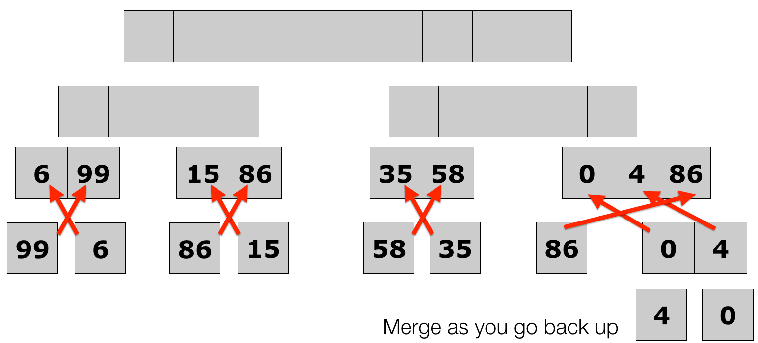
- How do you get initially sorted lists?
- Divide the list into half.
- Keep dividing each half until you are left with one element lists
- Because each list is only one element, it is, by definition, sorted
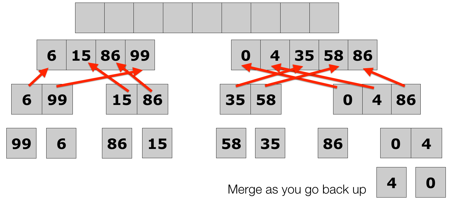
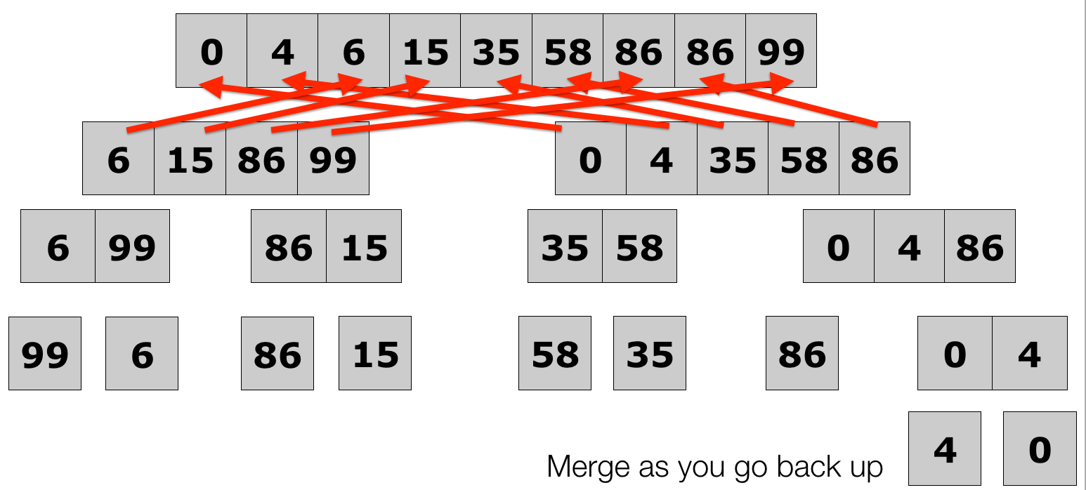
- Repeatedly merge the sublists together, two at a time, until there is only one sublist remaining. This will be a fully-sorted list.
def merge(lst1, lst2):
    """ Merge two already sorted lists and return the new, sorted list"""
    new_list = []
    len1 = len(lst1)
    len2 = len(lst2)
    p1 = 0
    p2 = 0
    while p1 < len1 and p2 < len2:
        if lst1[p1] <= lst2[p2]:
            new_list.append(lst1[p1])
            p1 += 1
        else:
            new_list.append(lst2[p2])
            p2 += 1

    new_list = new_list + lst1[p1:] + lst2[p2:]
    return new_list
Lecture 10: Merge Sort
- How do you get initially sorted lists?
- Divide the list into half.
- Keep dividing each half until you are left with one element lists
- Because each list is only one element, it is, by definition, sorted
- Repeatedly merge the sublists together, two at a time, until there is only one sublist remaining. This will be a fully-sorted list.
def merge_sort(lst):
    """ Use merge sort to sort lst in place"""
    n = len(lst)
    if n <= 1:
        return lst  # list with 0 or 1 elements is already sorted
    sublist1 = lst[:n // 2]
    sublist2 = lst[n // 2:]
    sublist1 = merge_sort(sublist1)
    sublist2 = merge_sort(sublist2)
    return merge(sublist1, sublist2)
Lecture 10: Merge Sort
- Merge sort full example
Lecture 10: Merge Sort
- Merge sort full example
Lecture 10: Merge Sort
- Merge sort full example
Lecture 10: Merge Sort
- Merge sort full example
Lecture 10: Merge Sort
- Merge sort full example

Lecture 10: Merge Sort
- Merge sort full example
Lecture 10: Merge Sort
- Merge sort full example
Lecture 10: Merge Sort
- Merge sort full example
Lecture 10: Merge Sort
- Merge sort full example
Lecture 10: Quick Sort
- Quicksort is a sorting algorithm that is often faster than most other types of sorts, including merge sort
- However, though it is often fast, it is not always fast, and can degrade significantly given the wrong conditions
- Quicksort is another divide and conquer algorithm
- The basic idea:
- Divide a list into two smaller sublists: the low elements and the high elements.
- Then, recursively sort the sub-lists
Lecture 10: Quick Sort
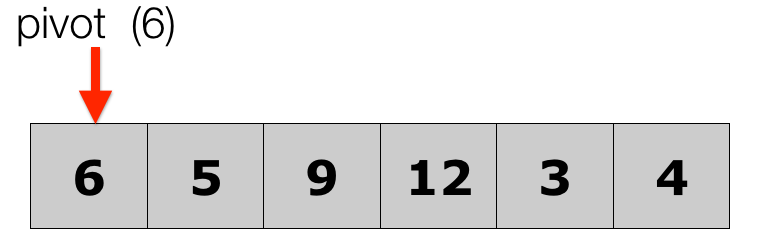
- The quicksort algorithm:
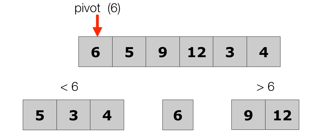
- Pick an element, called a pivot, from the list
- Reorder the list so that all elements with values less than the pivot come before the pivot, while all elements with values greater than the pivot come after it. After this partitioning, the pivot is in its final position. This is called the partition operation.
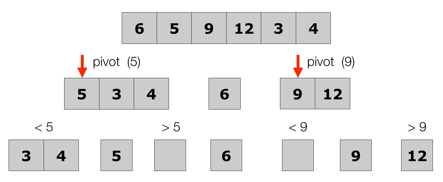
- Recursively apply the above steps to the sub-list of elements with smaller values and separately to the sub-list of elements with greater values.
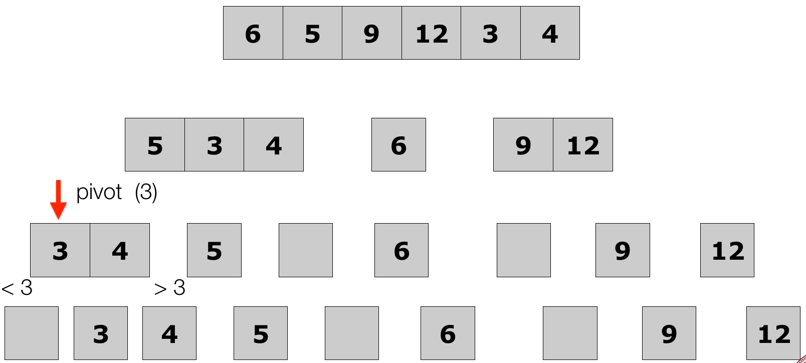
- The base case of the recursion is for lists of 0 or 1 elements, which do not need to be sorted.
Lecture 10: Quick Sort
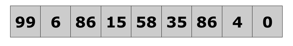
- Let's look at how we can run quick sort. The idea is to create new lists as we divide the original list.
- First, pick a pivot:
Lecture 10: Quick Sort
-
Partition into two new lists -- less than the pivot on the left, and greater than the pivot on the right.
Even if all elements go into one list, that was just a poor partition.
Lecture 10: Quick Sort
-
Keep partitioning the sub-lists
Lecture 10: Quick Sort
-
Keep partitioning the sub-lists
Lecture 10: Quick Sort
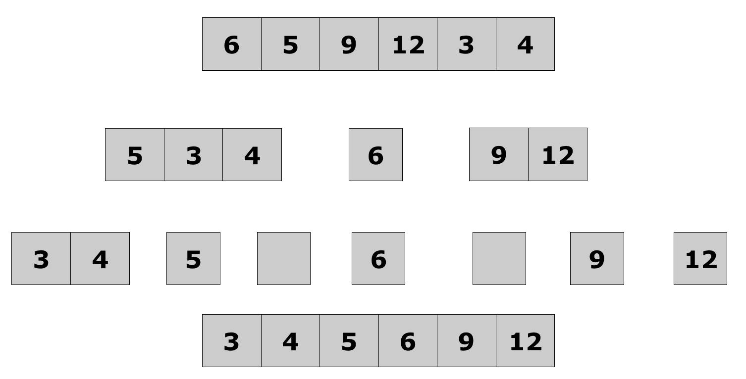
-
Keep partitioning the sub-lists
Lecture 10: Quick Sort
-
The quicksort functions:
def partition(lst, pivot):
    """ Partition a list into low and high elements, based on the pivot index"""
    pivot_val = lst[pivot]
    small_list = []
    large_list = []
    for i, value in enumerate(lst):
        if i == pivot:
            continue
        if value < pivot_val:
            small_list.append(value)
        else:
            large_list.append(value)
    return small_list, large_list

def quicksort(lst):
    """Perform quicksort on a list, in place"""
    if len(lst) <= 1:
        return lst
    # pick a random partition
    pivot = random.randint(0, len(lst)-1)
    small_list, large_list = partition(lst, pivot)
    return quicksort(small_list) + [lst[pivot]] + quicksort(large_list)