Applied Microeconomics
Lecture 3
BE 300
When Prices Change, How Will Consumers Respond?
From “Cosi is Good to Go” (August 2008):
RJ Dourney, owner of 13 Cosi franchises in the Boston area, has raised prices by 4 percent over the last year. Raising prices is always a suspenseful proposition, but it’s worked out well for Dourney. “I have seen no guest-count erosion,” says Dourney…
When Prices Change, How Will Consumers Respond?
From “Cosi is Good to Go” (August 2008) (cont):The 4 percent figure wasn't guesswork, Dourney based it on reports that franchisor Cosi Inc. commissions from Revenue Management Services, a Tampa Fla-based consulting firm.
"… the reports … tell you how much room you have in pricing before you start losing guests…"
Elasticity
The concept of elasticity measures how sensitive the quantity demanded is to a change in price.
When price changes, how much will the quantity demanded change?
Think of three products--"Not very sensitive", "Somewhat sensitive" and "Very sensitive" and why.
Elasticity
Some things that effect elasticity:
- Availability of close substitutes
- Necessities vs Luxuries
- Narrow vs. broadly defined markets
- Fraction of consumer's budget taken up by the good
Elasticity
One of the most commonly used measures of sensitivity of the demand curve is own price elasticity.
The own price elasticity of demand (ɛ): percentage change in the quantity demanded of a good for a 1 percent increase in its price.
What is the sign of ɛ?
Note: own-price elasticity of demand is (almost) always negative; but by convention, own-price elasticity of demand is often reported as its absolute value |Ep|.
Elasticity
Elasticity is calculated as:
ɛ = (Δ Q)/Q
(Δ P)/P
This can be written as:
ɛ= [ΔQ/ΔP] * (P/Q)
How is this related to our LINEAR graph of demand?
Elasticity
Two important things to note:
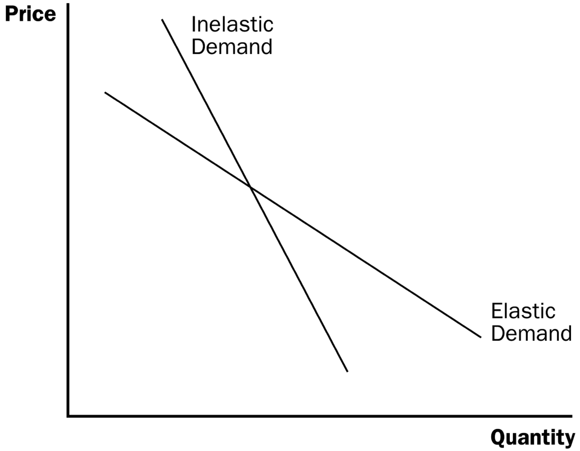
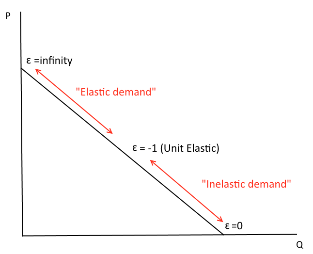
(1) Elasticity can be used to compare 2 different demand curves at the same point. The demand curve with the steeper slope is [MORE or LESS ?] elastic than the demand curve with the flatter slope.
(2) Elasticity changes as you move along the same demand curve--some parts of the demand curve are more elastic.
Elasticity
Elasticity
O2, Brute?
Case Objectives:
We have four objectives:
- Estimating demand by deriving a linear demand curve from data observations.
- Calculating own-price elasticity of demand using the point formula.
- Illustrating the relationship between elasticity & total revenue.
- Analyzing the resulting P & Q from movement along vs. shifts of demand curves.
Estimating Demand
Informal or Back-of-the-envelope estimation
- We can infer a linear demand from just two observations (two locations at a point in time, or data from two time periods, e.g., two consecutive weeks or years)
- We can infer demand from knowledge of current sales and prices, and published elasticities
You will see and example of inferring demand
from two observations in today’s case
Estimating Demand
Formal (i.e., statistical) approach:
- Use multiple regression analysis to estimate lines (or curves) through data points.
- Again the data can be time series (units sold and prices over time) or cross market (units sold and prices in different cities, or zip codes, etc.)
We’ll work with an example of a statistically
estimated demand curve in the Tagamet case.
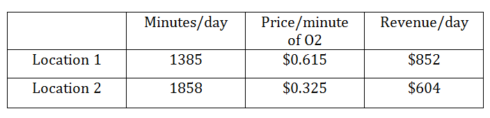
Oxygen Bar Data
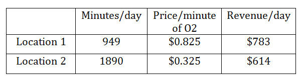
Observation: Despite a higher price and lower volume, Location 1 generates more revenue.
Is there a "better" average price for Location 2, i.e., one that would yield higher revenue? And Location 1?
O2, Brute?
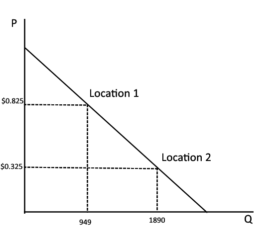
Let's assume these are two points on the same demand curve. We can use data in the table to derive a linear demand curve.
We think of the demand curve as P=M*Q+B.
How do you find the slope (M)?
O2, Brute?
Let's assume these are two points on the same demand curve. We can use data in the table to derive a linear demand curve.
We think of the demand curve as P=M*Q+B.
How do we find the y-intercept (B)?
O2, Brute?
For the inverse demand curve (the one with P on the left hand side), the slope is change in P over change in Q:
M=(0.825-0.325)
(949-1890)
M= -0.0005 (rounding)
To find the intercept, plug in the slope and two of the points:
0.825=(-0.0005)*949+b implies b=1.3 (rounding)
P=1.3 - 0.0005 Q
O2, Brute?
We can use the same method to find the equation for the regular (not inverse) demand curve:
M=(ΔQ/ΔP)=(949-1890)/(0.825-0.325)=-1882
Q=B-1882*P
Plug in a point:
949=B-1882*(0.825)
B=2501.65
Q=2501.7-1882P
(or just solve for Q using the inverse demand curve)
O2, Brute?
O2, Brute?
Location I : Could revenue be increased by changing price
and, if so, in which direction?
Assume these points are on the same demand curve!
Using Demand Equations for Business Decisions
One reason that we are interested in demand is because it tells
us how quantity demanded (or sales) is likely to change as we
change price, and price and quantity together determine revenue:
TR = P*Q
- Raising price will be more desirable if quantity falls only a little bit when we raise price.
- Lowering price will be more attractive to the extent that quantity increase a lot when we lower price.
Using Demand Estimation for Business Decisions
“If you set the price too high, then your sales are too low but if you set the price too low, margins are squeezed and we run out of inventory.” --“How Sears Uses Big Data to Get a Handle on Pricing” (WSJ, June 2012)
How do we know how to balance price with quantity?
By understanding how sensitive our demand is to a change in price.
Elasticity
Recall: elasticity is %change in Quantity Demanded divided by %change in price. I.e:
ɛ = (Δ Q)/Q
(Δ P)/P
In the linear demand curve case, (ΔQ/ΔP) is constant--what is it in the Oxygen Bar example?
-1882
Recall: for the linear demand curve, ɛ is (1/slope)*(P/Q).
Elasticity
We categorize elasticity into one of three groups:
Inelastic (price insensitive) if |ɛ| < 1
1% change in P causes less than a 1% change in Q demanded.
Elastic (price sensitive) if |ɛ| > 1
1% change in P causes more than a 1% change in Q demanded.
Unit elastic if |ɛ|=1
1% change in P causes exactly a 1% change in Q demanded.
Elasticity
“Americans Start to Curb Their Thirst for Gasoline”
(WSJ, Mar 3, 2008):
“A 10% rise in gasoline prices reduces consumption by just
0.6% in the short term...”
What does this imply about the short-term price elasticity for
gasoline? Is the demand for gasoline elastic, inelastic, or unit elastic?
Elasticity
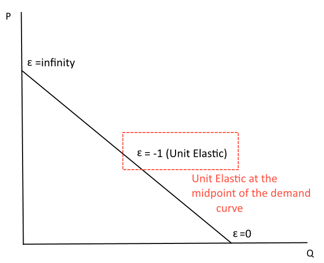
Elasticity is not the same thing as slope!
Elasticity
Elasticity
What is the elasticity of demand at Location 1?
What is the elasticity of demand at Location 2?
Elasticity
So, why should we care about elasticity?
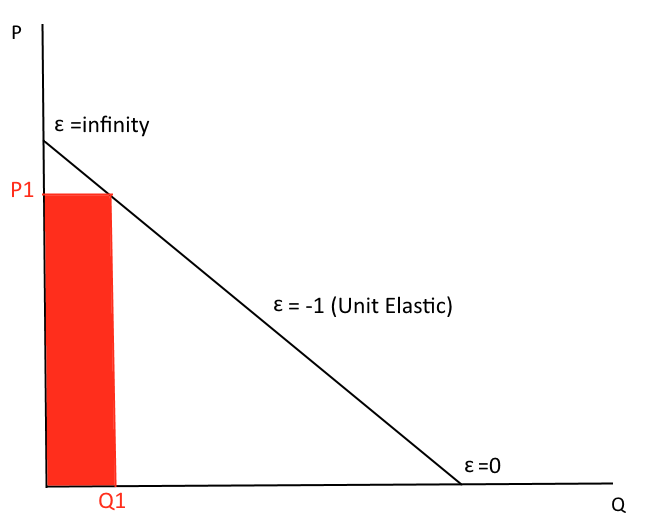
A change in price has a different effect on revenue depending on the elasticity at that point!
Elasticity
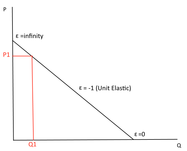
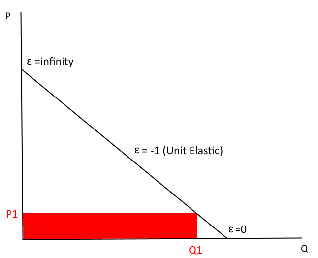
Say we're at P1. Where is revenue? Is demand elastic, inelastic, or unit elastic at this point?
Elasticity
Now, we increase the price a bit...
Elasticity
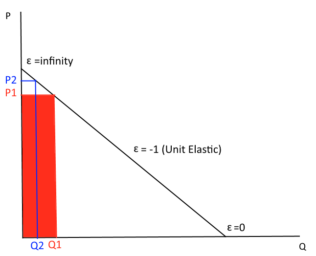
Elasticity
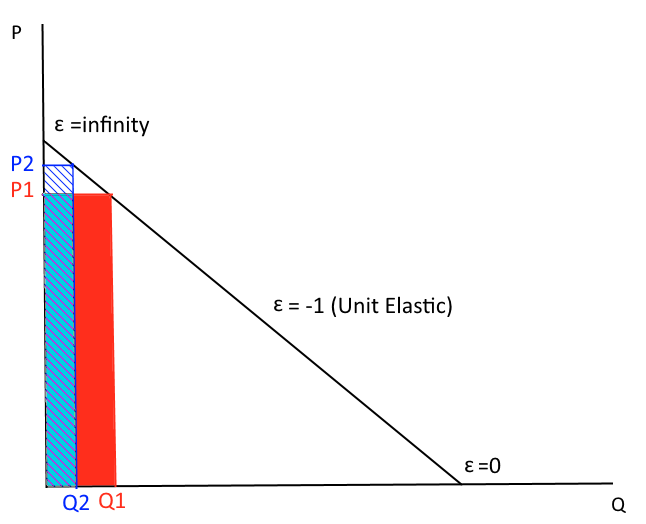
Total revenue falls
Elasticity
Increasing price in the "inelastic" area of the demand curve...
Elasticity
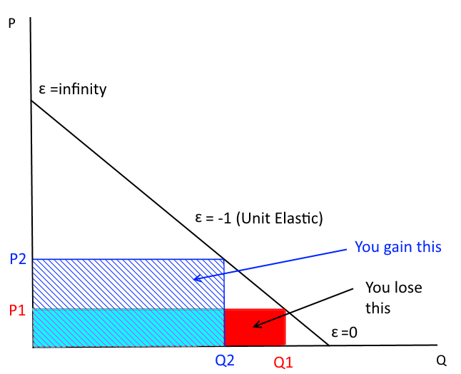
Revenue goes up
Elasticity
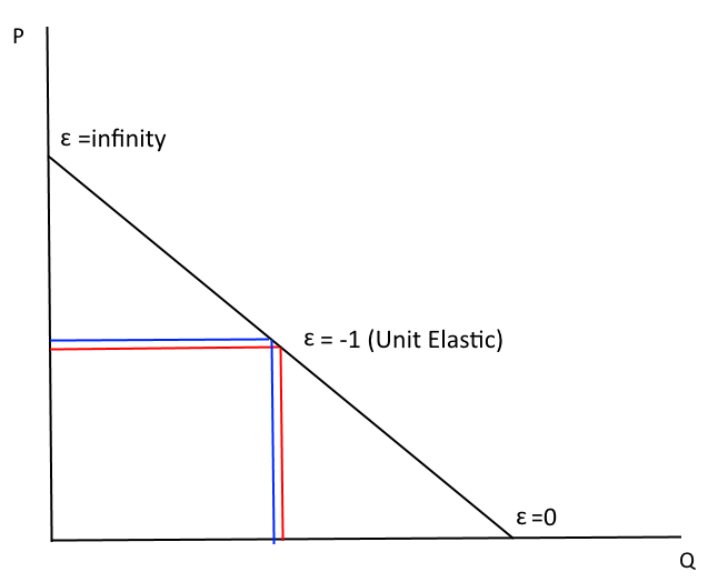
At the midpoint--the gains and losses cancel each other out. No change in revenue.
Elasticity
Inelastic (price insensitive) if |e| < 1; If price increases, then total revenue rises
Elastic (price sensitive) if |e| > 1; If price increases, then total revenue falls
Unit elastic if |e| = 1; If price increases or decreases, then total revenue is unchanged
Elasticity
Failing to account for this may lead to incorrect business decisions.
Elasticity
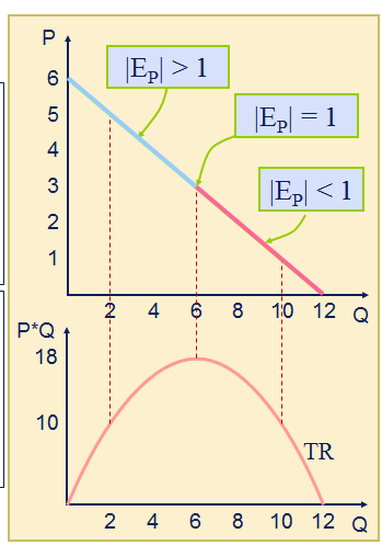
Since P and Q are linked, you can also think of this as the relationship between Q and total revenue
Elasticity
Practice question:
In the agricultural equipment industry of developing nations, firms in recent years have benefited from the introduction of new technology. An industry spokesperson was heard to say, "This new technology is actually a mixed blessing. With it, firms in our industry will produce so much machinery that price and industry revenues will probably fall!" This spokesperson must be assuming that, at prevailing prices and quantities,
- the demand for machinery is inelastic
- the demand for machinery is elastic
- the demand for machinery is unit elastic
- not enough information
O2, Brute?
Back to the case:
Is the proposed solution "correct" (i.e., is a price of $.65 per minute O2 the revenue maximizing price)?
O2, Brute?
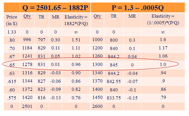
Short cut:1. Estimated Demand Curve: Q = 2501.65 – 1882P
2. When P = 0; Q = 2501.65 => Q midpoint = 1250.8
3. When Q=0; P = 1.33 => P midpoint = $.665
or:
1. Estimated Inverse Demand Curve: P = 1.3 – .0005Q
2. When P = 0; Q = 2600 => Q midpoint = 1300
3. When Q = 0; P = 1.30 => P midpoint = $.65
(Differences come from rounding)
O2, Brute?
O2, Brute?
(Question 3): The CEO runs an experiment where he lowers the price of O2 per minute at Location 1 to $0.615 per minute and keeps price at Location 2 the same. This is the result:
O2, Brute?
When prices were changed at Location 1, revenue rose to $852 at an average price of $0.615 per minute O2. Yet, using the estimated demand curve, revenue at a price of $0.615 should have been $842.55. How could the actual revenue earned have exceeded both the predicted revenue figure and the theoretical revenue maximum?
O2, Brute?
Should the CEO consider changing prices at location 2? Why or why not?
Demand Estimation: Summary
The O2, Brute? case demand curve “estimation” illustrates an informal, “back-of-the-envelope” approach using very limited data — just 2 observations or “data points”
However, the underlying principles — and the potential problems — are the same for more sophisticated methods of estimating demand
Required Inputs for Demand Estimation:
- Data
- Methods to analyze the data
Demand Estimation
The demand curve is the relationship between how much of a product a person buys (Qd) and its price (P), everything else constant.
Companies estimate and forecast demand for their products all the time to answer questions such as:
- what will happen if I decrease my price by 5%?
- what will happen if my competitor decreases price by 1%?
- what if I increase my advertising budget by 10%?
Demand Analysis
An elasticity is the percentage change in one variable (usually quantity) divided by the percentage change in another variable (e.g., own price, income, price of a substitute or complement)
- Own-price elasticity of demand describes sensitivity of demand to price changes, in percentage terms.
- The own-price or “demand” elasticity = %ΔQ/%ΔP
- Various factors affect the own-price elasticity of demand, including include the number of substitutes, the share of consumer’s revenues that goes to a product, the time frame (short or long run), etc.
Elasticity
Critical link between price sensitivity, pricing decisions, and revenue implications
- When demand is elastic (at going prices and quantities) decreasing price leads to higher revenues;
- When demand is inelastic, price increases lead to higher revenues.
NOTE: revenue ≠ profit!
For Next Time: Tagamet Case
Hint for working on the Tagamet Case:
- Work through practice problems 4 & 5 in the practice problems (on Ctools site) before tackling the case; problems 8 & 9 are similar to the Tagamet case questions
- Review the following problem (in slide deck following this slide)*
- Income and Cross-Price Elasticities explained in textbook, p. 50-52
* (taken from Pindyck & Rubinfeld, Microeconomics, 5th ed.)
Hints for Tagamet
Suppose that you are the consultant to an agricultural cooperative that is deciding whether members should cut their production of cotton in half next year. The cooperative wants your advice as to whether this action will increase members’ revenues.Knowing that cotton (C) and watermelon (W) both compete for agricultural land in the South, you estimate the demand for cotton to be C = 3.5 – 1.0Pc + 0.25Pw + 0.50I, where Pc is the price of cotton, Pw is the price of watermelon, and I income.
Should you support or oppose the plan? Is there any additional information that would help you to provide a definitive answer?
Hints for Tagamet
C = 3.5 – 1.0Pc + 0.25Pw + 0.50I
- Should you support or oppose the plan to cut production of cotton in half?
- First, calculate the own-price elasticity of demand for cotton: E=(∆Pc/∆Qc)*(Qc/Pc)
- From equation, ∆Qc /∆Pc = -1.0 => E= -1.0*(Pc/Qc)
- If (Pc/Qc) > 1, demand will be elastic, so when Qc ↓ (and Pc ↑), TR from cotton falls
- If (Pc/Qc) = 1, demand will be unit elastic, so when Qc ↓ (and Pc ↑), TR from cotton stays the same
- If (Pc/Qc) < 1, demand will be inelastic, so when Qc ↓ (and Pc ↑), TR from cotton increases
Hints for Tagamet
Is there any additional information that would help you to provide a definitive answer?
You certainly would want to know Pc & Qc so you could calculation own-price elasticity for cotton
But... what about watermelon?
You may also want the data necessary to understand the demand function (and elasticity) of watermelon (e.g., Pw, Qw) IF cooperative members’ revenues depend on revenue from both watermelon AND cotton.
Next Time
Tagamet Case is due
Read about Regression Analysis: Ch. 3.2 – 3.5