Mechanical Engineering, Carnegie Mellon University
Advisors: Prof. Burak Kara, Prof. Jessica Zhang
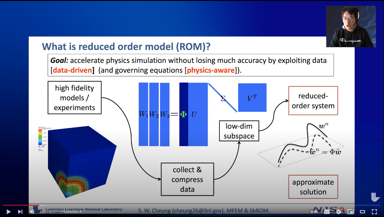
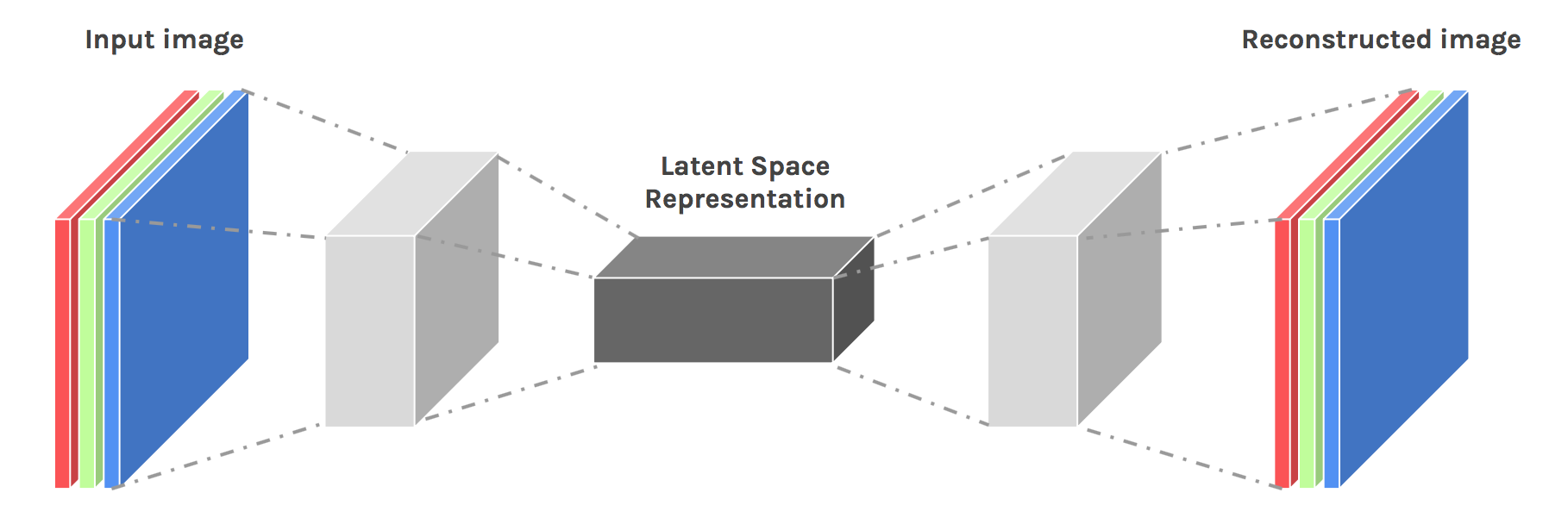
Reduced Order Modeling
- Accelerate physics simulations without losing much accuracy
- Take supercomputer-scale problems, and reduce them to laptop scale
Offline
Compute cost immaterial
Online
Must be cheap to run
Collect high-fidelity data
Precompute reduced model
Evaluate model
Reduced Order Modeling Considerations
We are concerned with

- Finding an optimal compression space
- Accurate, stable time evolution
- Use less data/ fast solve cheap
- We are not concerned with boundary handling
- High Reynolds number, advection-dominated flows
- Numerical experiments:
- 1D, 2D Burgers equation in a periodic box with \(\mathit{Re}=10,000\)
- SOTA: 10x speedup, <1% relative error
Target application
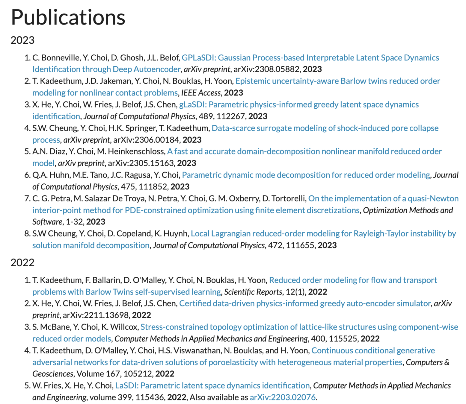
Extensive literature on ROM (traditional/ ML approaches)
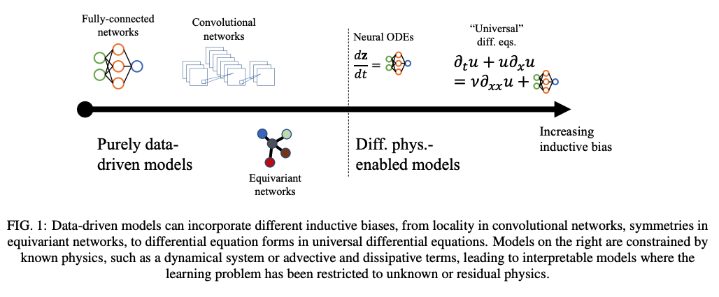
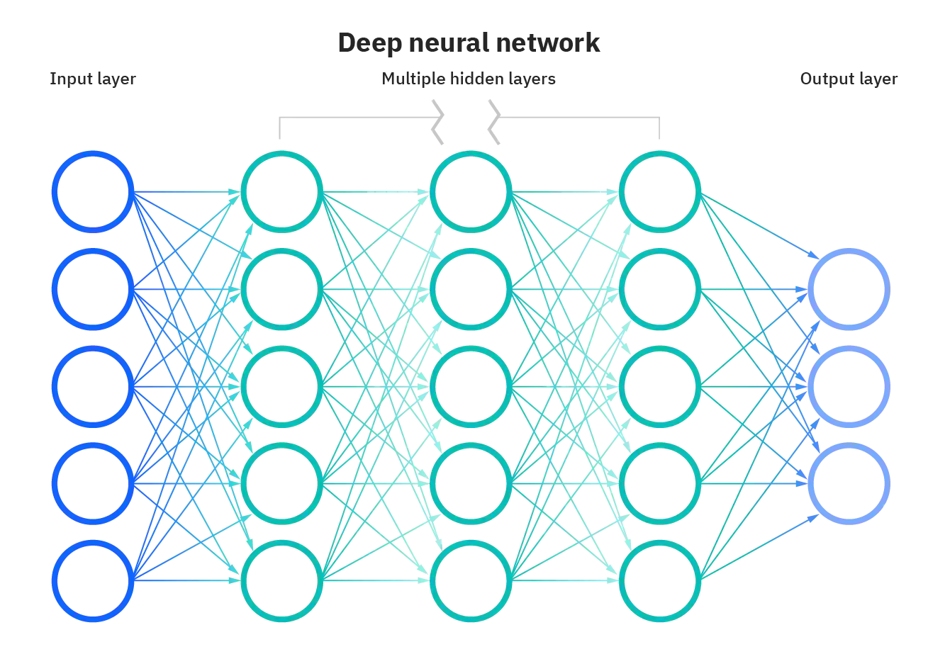
Landscape of ML for PDEs
Mesh-based
PDE-Based
Neural Ansatz
Data-driven
FEM, FVM, IGA, Spectral
Fourier Neural Operator
Implicit Neural Representations
DeepONet
Physics Informed NNs
Convolution NNs
Graph NNs
Adapted from Núñez, CEMRACS 2023
Neural ODEs
Universal Diff Eq
Hybrid Phys/ML
Reduced Order Modeling
Reduced Modeling Approaches
Increasing inductive bias
Data-driven/ black-box
Principal Component Analysis
Learned dynamics
Physics-based dynamics
Neural surrogate
ML based latent space
Closure Modeling
Reduced Modeling Approaches
Increasing inductive bias
Data-driven/ black-box
Principal Component Analysis
Learned dynamics
Physics-based dynamics
Neural surrogate
ML based latent space
Closure Modeling
PCA: compute basis from data
Singular Value Decomposition

On closures for reduced order models—A spectrum of first-principle to machine-learned avenues, Ahmed et al. Phys of Fluids, 2021
Apply learned mapping \(u(x, t) = \Phi_n \cdot \tilde{u}\) to PDE
- Nonlinear term needs to be evaluated in full-order space
- Improper handling of nonlinearity leads to stability problems
- Linear models, i.e. \(u(x, t)= \sum_i \tilde{u_i}(t)\phi_i(x) \), shown to have limited approximation capability
- Not suitable for advection dominated problems (eg. turbulent flows)
Reduced Modeling Approaches
Increasing inductive bias
Data-driven/ black-box
Principal Component Analysis
Learned dynamics
Physics-based dynamics
Neural surrogate
ML based latent space
Closure Modeling
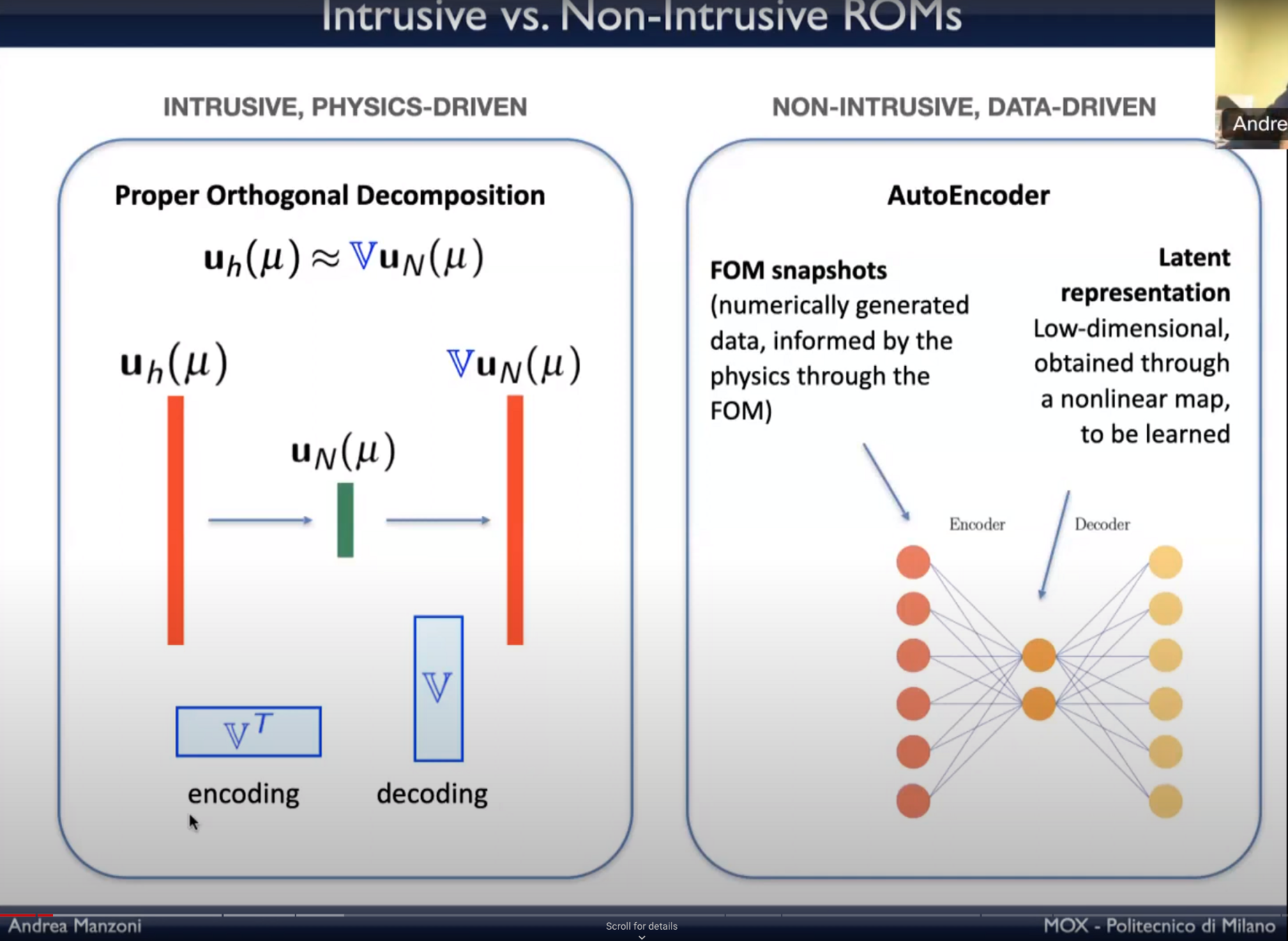
Comparing POD and auto-encoders
ML Based purely data-driven approach
- Learn nonlinear latent space from snapshot data with autoencoders
- Learn dynamics in latent space
- Purely data-driven approaches extrapolate poorly to unseen parameters
Reduced Modeling Approaches
Increasing inductive bias
Data-driven/ black-box
Principal Component Analysis
Learned dynamics
Physics-based dynamics
Neural surrogate
ML based latent space
Closure Modeling
Nonlinear Manifold ROM Challenges/ Research
- NM-ROM have much higher offline cost
- Jacobian evaluation \( \dfrac{\partial d}{\partial \tilde{u}} \) makes online solve very slow
- Decoder size scales with full-order-model size
- Need to make decoder size independent of full-order-model
- Many encoding methods exist
- Hard to find optimal latent-space size, hyper-reduction points
- Current works resort to hyper-parameter tuning
- Potential opportunity to make it dynamic
| Encoding Architectures |
|---|
| (Variational) Auto-encoder |
| (Variational) Auto-decoder |
| Implicit Neural representations |
| Dynamic weights |


NM-ROM State of the Art
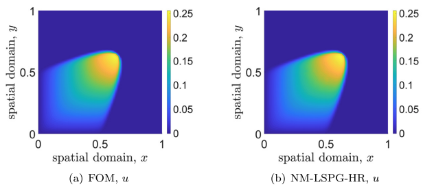
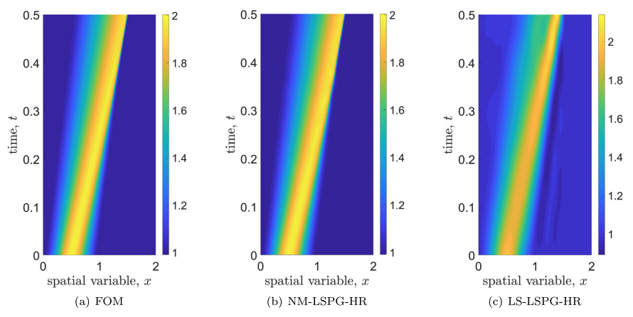
Results from 2D Burgers' problem, \(\mathit{Re} = 10,000\) (\(11\times\) speedup)
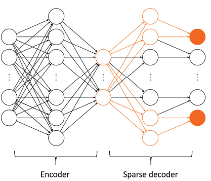
Shallow, masked auto-encoder
In follow up work (May 2023), the authors combined shallow encoders with domain decomposition methods.
Challenges
ML based Nonlinear-Manifold Reduced-Order-Modeling
Nonlinear manifold latent space with ML
Petrov-Galerkin
time-evolution
| Challenge | Possible Research Directions |
|---|---|
| Use of small autoencoders | Use novel encoding methods (implicit neural representations (INR)) |
| Fixed latent space size | Develop Fourier based auto-encoder that can adjust latent-space size. Behaves similarly to convolutional autoencoder |
| Fixed hyper-reduction points | INR allows for sampling at any point |
| Autoencoder training too expensive | - Attempt pre-training / fine-tuning methodology - Attempt auto-decoder architectures |
| Reduce data dependence | Explore over-fitting with dynamic-weights methdos |
- Nonlinear manifold obtained from data
- Time-evolution with numerical methods
- New field: ~10 papers out
- Many challenges, many research directions
- Each choice of architecture leads to a unique tradeoff in time-integrator, solver choice, hyper-reduction scheme
NM-ROM Paper Comparison
| Paper | Method | Description |
|---|---|---|
|
NM-ROM Deep CAE Carlberg, 2020 |
Latent space: deep conv auto-encoder Time: equation based (PG-HR) |
First work combining ML latent space with physics based dynamics. Slow online solve due to high cost of Jacobian computation. Examples: 1D inviscid Burgers |
|
NM-ROM Shallow CAE Kim, 2022 |
Latent space: shallow conv auto-encoder Time: equation based (PG-HR) |
Replace deep CAE with shallow CAE to speed up online solve Examples: 1D/2D viscous Burgers, Re = 10k |
|
Neural Implicit Flow Burton, 2022 |
Space/time: implicit neural field | Full surrogate model Examples: 1D KS, 2D NS (Rayleigh-Taylor instability), isotropic turbulence |
|
Continuous ROM Chen, Carlberg, 2023 |
Latent space: implicit neural field Time: equation based (PG-HR) |
No online dependence on full-order-model size. Examples: 1D inviscid Burgers, NS (vortex shedding), nonlinear elasticity |
|
Dynamic Weights Nunez, 2023 |
Latent space: dynamic weights Time: data-driven |
Latent space given by weights of NN. Learns neural ODE to evolve network weights. Examples: 1D Burgers, 1D KdV, 1D KS |
|
Deep-HyROMnet Manzoni, 2023 |
Latent space: implicit neural field Time: equation based (PG-HR) |
Train neural-network to do hyper-reduction |
Mechanical Engineering, Carnegie Mellon University
Advisors: Prof. Burak Kara, Prof. Jessica Zhang
Reduced Modeling Approaches
Increasing inductive bias
Data-driven/ black-box
Principal Component Analysis
Learned dynamics
Physics-based dynamics
Neural surrogate
ML based latent space
Closure Modeling
Reduced Modeling Approaches
Increasing inductive bias
Data-driven/ black-box
Principal Component Analysis
Learned dynamics
Physics-based dynamics
Neural surrogate
ML based latent space
Closure Modeling
- Learn spatial discretization with ML
- Evolve PDE with time-integrators
Nonlinear Manifold Reduced Order Modeling
- Manipulate system to make it solvable (hyper-reduction)
- Such techniques fall under Petrov-Galerkin projection method
- Solve with least squares/ rootfinding to evolve in time
- Train encoder-decoder on snapshots
- Apply learned mapping to PDE
- Evolve with time-integrators
Lee, Carlburg, Model reduction of dynamical systems on nonlinear manifolds using deep convolutional autoencoders, J. Comp. Phys, 2019
ML Based purely data-driven approach
- Learn nonlinear latent space from snapshot data with autoencoders
- Learn dynamics in latent space
- Purely data-driven approaches extrapolate poorly to unseen parameters
NM-ROM Challenges, Ideas
| Challenges | Possible Research Directions |
|---|---|
| Expensive Training | - Use novel encoding methods in place of auto-encoder - Attempt pre-training / fine-tuning methodology - Attempt auto-decoder architectures |
| Reduce data dependence | - Explore over-fitting with dynamic-weights methods |
| Fixed latent space size | Develop Fourier based auto-encoder that can adjust latent-space size |
- Learn nonlinear trial space from data
- Test space based on over-collocation
- Evolve with time-integrators
-
Proposal: Fourier-based encoding
- Faster training compared to conv auto-encoders
- Possibly adjustable latent space size
- Pre-train on general datasets will lead to fewer problem
NM-ROM Paper Comparison
| Paper | Method | Description |
|---|---|---|
|
NM-ROM Deep CAE Carlberg, 2020 |
Latent space: deep CAE Time: equation based (PG) |
Solve dynamical system where space discretization is given by NN. Online solve depends on FOM size. |
|
NM-ROM Shallow CAE Kim, 2022 |
Latent space: shallow CAE Time: equation based (PG-HR) |
Replace deep CAE in NM-ROM Deep CAE with shallow network. Online solve independent of on FOM size thanks to hyper-reduction. |
|
DL-ROM Manzoni, 2020 |
Latent space: CAE Time: deep NN |
Surrogate model inside an AE bottleneck. Can be queried at any point w/o time-evolution |
|
Deep-HyROMnet Manzoni, 2023 |
Latent space: implicit neural field Time: equation based (PG-HR) |
Train neural-network to do hyper-reduction |
|
Neural Implicit Flow Burton, 2022 |
Space/time: implicit neural field | Full surrogate model can be queried at any time w/o requiring a dynamic system solve |
|
Continuous ROM Chen, Carlberg, 2023 |
Latent space: implicit neural field Time: equation based (PG-HR) |
No online dependence on full-order-model size |
|
Dynamic Weights Nunez, 2023 |
Latent space: dynamic weights Time: data-driven |
Latent space given by weights of NN. Learns neural ODE to evolve network weights. |
| Proposal 1 |
Latent space: Fourier AE, INR Time: equation-based (PG-HR) |
Fourier based encoder, INR based decoder. |
Comparison with literature
| NM ROM D | NM ROM S | DL-ROM | Deep-HyROM | NIF | CROM | DW | Proposal 1 | |
|---|---|---|---|---|---|---|---|---|
| Nonlinear latent space | Y | Y | Y | Y | Y | Y | Y | Y |
| Data => latent space | Y | Y | Y | Y | Y | Y | Y | Y |
| Expensive training | Y | Y | Y | Y | Y | Y | Y | Y |
| Autoencoder slows down online solve | Y | Y | N | N | N | N | N | N |
| Fixed latent space size | Y | Y | Y | Y | Y | Y | Y | N |
| Equation-based dynamics | Y | Y | N | Y | N | Y | N | Y |
| Fixed latent space size | Y | Y | Y | Y | Y | |||
| Fixed hyper-reduction points | - | N | - | N | - | Y | - | Y |
- Proposal 1: Fourier-based encoding
Plan
Title: Fourier-based auto-encoders for Nonlinear Manifold Reduced Order Modeling.
Possible new contributions
- In the literature, people used conv auto-encoders
- Fourier-based encoder should be faster to train that convolutional encoders, higher accuracy
- Can possibly adjust latent-space size
Plan
- Data Generation (1 day)
- 1D/ 2D Burgers problem, \(\mathit{Re}=1k - 10k\)
- Model Implementation
- Latent space (1 week)
- Read up on auto-encoders (2-3 days)
- Implement model (2-3 days)
- Time evolution (1 week)
- Implement time-evolution schemes
- Latent space (1 week)
- Numerical Experiments
- Train model on Burgers' data
Mechanical Engineering, Carnegie Mellon University
Advisors: Prof. Burak Kara, Prof. Jessica Zhang
Updates 9/29/23
Title: Fourier-based auto-encoders for Nonlinear Model Order Reduction.
Possible new contributions
- In the literature, people used conv auto-encoders for learning ROM latent spaces
- Claim: Richer auto-encoder representation can lead to a smaller latent space size.
- Fourier-based encoder should be faster to train that convolutional encoders, higher accuracy
- Hope: can possibly adjust latent-space size
Updates
- Generated 1D Burgers data
- Training auto-encoder models
Notes from discussion
- Look into topology optimization + NM-ROM.
Plan
- Data Generation (1 day) [done]
- 1D/ 2D Burgers problem, \(\mathit{Re}=1k - 10k\)
- Model Implementation
- Latent space (2 week)
- Read up on auto-encoders (2-3 days)
- Implement model (2-3 days)
- Time evolution (2 week)
- Implement time-evolution schemes
- Latent space (2 week)
- Numerical Experiments
- Train model on Burgers' data
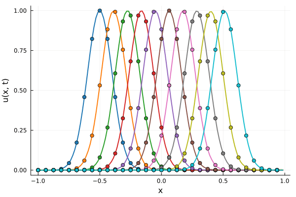
Data Generation
- 1D Viscous Burgers', Re = 10,000 on N = 1024 point grid
- 100 trajectories trained on randomly generated initial conditions
- 100 snapshots between T=0-10.
- Total 10k snapshots \(\cdot\) 1024 points per snapshot = \( 1.2\cdot 10^7\) points
First autoencoder implementation
Training Trajectory
Test Trajectory
- Train a simple auto-encoder model on Burgers data
- Train on T=0-5s on selected trajectories, test on T=0-10s
- 5% relative error on both test/train sets
[WIP] Compare with experiments
Kim et al, A fast and accurate physics-informed neural network reduced order model with shallow masked autoencoder. J. of Comp. Phys
- Previous experiment had much more complicated and varying signals.
- This makes autoencoder training hard and introduces the need for a large latent space.
- Here, I am attempting to compare with experiments from literature.
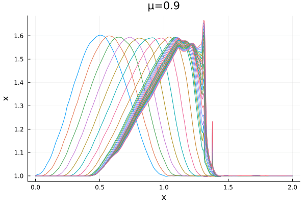
- Target problem: inviscid Burgers with varying initial condition.
- The variable \(\mu\) is to be varied in range \([0.9, 1.1]\).
Updates 10/03/23
Title: Fourier-based auto-encoders for Nonlinear Model Order Reduction.
Learned latent space with auto-encoders, equation-based time-evolution
Literature Review
- In literature, people used convolutional auto-encoders (AEs).
- Drawbacks: large training cost, large online solve cost
- Some work has been done on other encoding methods
- Another challenge is to have a variable latent-space size
Possible new contributions
- Fourier-based encoder should be faster to train that convolutional AEs
- Richer AE representation can lead to a smaller latent space size
- Adjust latent space size with mix of linear + nonlinear reduction
Updates
- Generated training data in line with experiments from literature
- Trained auto-encoder models
- Next: implement time-evolution schemes
Topology optimization: Lit review on level set method. Meeting with Prof. Kara.
Plan
- Data Generation (1 day)
- 1D/ 2D Burgers problem, \(\mathit{Re}=1k - 10k\)
- Model Implementation
- Latent space (2 week)
- Read up on auto-encoders (2-3 days)
- Implement model (2-3 days)
- Time evolution (2 week)
- Implement time-evolution schemes
- Latent space (2 week)
- Numerical Experiments
- Train model on Burgers' data
Experiment in literature
Kim et al, A fast and accurate physics-informed neural network reduced order model with shallow masked autoencoder. J. of Comp. Phys
- Target problem: inviscid Burgers with varying initial condition.
- The variable \(\mu\) is to be varied in range \([0.6, 1.2]\).
Data - Burgers' problem
- Inviscid burgers is a hard to solve for large \(\mu\) due to the presence of shocks
- So we add a small amount of viscosity \(1/\nu=10,000\) to stabalize the system

First autoencoder implementation
Training Trajectory
Test Trajectory
- Train on \(\mu = \{0.6, 0.9, 1.2\}\), test on \(\mu = \{0.7,0.8, 1.0, 1.1\}\)
- 2% relative error on training set, 7% on test set
New Ideas
Nonlinear Reduction
- decoder= mixed linear (courier) + nonlinear (inr hyper network)
- decoder = hyper network with multiple levels of training
would be interesting to look at multil|evel nn on sirens.
equivalent on getting pca modes is training a new autoencoder with boosting?
Topology Optimization
- Combine Hamilton-Jacobi paradigm with Aditya's PINNs work
- Apply model reduction to solve topology optimization HJ equations
Updates 10/06/23
Topic: Learned latent space with auto-encoders, equation-based time-evolution
Title: Fourier-based auto-encoders for Nonlinear Model Order Reduction
Literature Review
- Most works use convolutional auto-encoders (AEs). Some use new methods
- Drawbacks: large training cost, large online solve cost
- Challenge: robustness of methods
- Challenge: changing latent space requires expensive re-training
Possible new contributions
- Speed up AE training with Fourier representations
- Richer AE representation can lead to a smaller latent space size
- Adjust latent space size with sequence of trained models
Updates
- Experiment and compare auto-encoder models
- Implement new encoding methods
Topology optimization
- Lit review on Machine Learning + Topology Optimization
- Meeting with VDEL Lab students (Ray, Aditya) on Monday (10/9)
Plan
- Data Generation (1 day)
- 1D Burgers problem, \(\mathit{Re}=10k\) [done]
- 2D Burgers problem, \(\mathit{Re}=10k\)
- Model Implementation
- Latent space (2 week)
- Read up on auto-encoders (2-3 days)
- Implement model (2-3 days)
- Time evolution (2 week)
- Implement time-evolution schemes
- Latent space (2 week)
- Numerical Experiments
- 1D/2D Burgers problem
- 2D Advection equation
Dataset
Kim et al, A fast and accurate physics-informed neural network reduced order model with shallow masked autoencoder. J. of Comp. Phys
- Add a small amount of viscosity \(1/\nu=10,000\) to stabalize the system
- Train on \(\mu = \{0.6, 0.9, 1.2\}\)
- Test on \(\mu = \{0.7,0.8, 1.0, 1.1\}\)
- \(N = 1024\) training points
- 100 snapshots per trajectory

Model Reduction Methods
Principal Component Analysis (Traditional)
Singular Value Decomposition
Convolutional Autoencoders
On closures for reduced order models—A spectrum of first-principle to machine-learned avenues, Ahmed et al. Phys of Fluids, 2021
| Method | ||||
|---|---|---|---|---|
|
|
||||
|
|
||||
|
|
||||
|
|

\(\mu=0.6\) (Train)
\(\mu=0.7\) (Test)
\(\mu=1.2\) (Train)
\(\mu=1.1\) (Test)


Implicit Neural Representation
Encoder/decoder (60k, 3k params)
Latent space size: 4
Convolutional Auto-Encoder
Encoder/decoder (60k, 60k params)
Latent space size: 16
Principal Component Analysis
Projection modes: 32
Principal Component Analysis
Projection modes: 16
Implicit Neural Representations
CROM: Continuous Reduced-ORrder Modeling of PDEs using Implicit Neural Representations, Int'l Conference on Learning Representations, 2023
Implicit Neural Representation allow for smaller latent-space size with equivalent representation capacity.
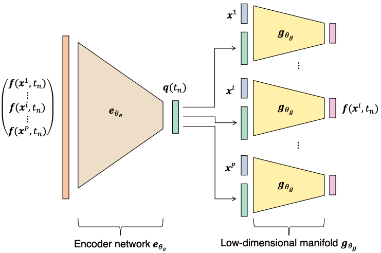
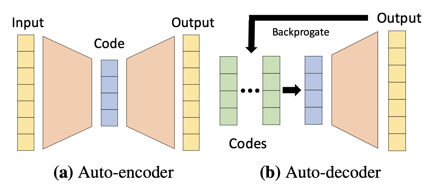
Auto-decoder: encoder-free learning
Park et al., DeepSDF: Learning Continuous Signed Distance Functions for Shape Representations, 2019
CROM: Continuous Reduced-ORrder Modeling of PDEs using Implicit Neural Representations, Int'l Conference on Learning Representations, 2023
Updates 10/09/23
Topic: Learned latent space with auto-encoders, equation-based time-evolution
Title: Making Nonlinear Model-Order Reduction robust and cheap
Literature Review
- Most works use convolutional auto-encoders (AEs)
- Challenge: large training cost, large online solve cost
- Challenge: robustness of methods
- Challenge: changing latent space requires expensive re-training
Possible new contributions
- Speed up training time for SOTA models (few hrs to few minutes)
- Apply method to larger problems with complex physics
- Richer AE representation can lead to a smaller latent space size
- Adjust latent space size with sequential model training
Updates
- Experiment and compare auto-encoder models
- Implement new encoding methods
Topology optimization
- Meeting with VDEL Lab students (Ray, Aditya) on Monday (10/9)
Plan
- Data Generation (1 day)
- 1D Burgers problem, \(\mathit{Re}=10k\) [done]
- 2D Burgers problem, \(\mathit{Re}=10k\)
- Model Implementation
- Latent space (2 week)
- Read up on auto-encoders (2-3 days)
- Implement model (2-3 days)
- Time evolution (2 week)
- Implement time-evolution schemes
- Latent space (2 week)
- Numerical Experiments
- 1D/2D Burgers problem
- 2D Advection equation
Nonlinear Reduction - Training Cost
| Paper | Method | Contribution | Model training | Online solve |
|---|---|---|---|---|
|
Conventional Approach |
Latent space: Apply PCA to data Time: equation based (PG-HR) |
Learn (linear) reduced representation via PCA. Evolve compact dynamical system | Apply SVD to data matrix Time: <2s |
Evolve dynamical system by minimizing residual at some points (Hyper-Reduction) |
|
NM-ROM Deep CAE Carlberg, 2020 |
Latent space: deep CAE Time: equation based (PG) |
Solve dynamical system where space discretization is given by NN. | Deep Conv. Auto-Encoders CNN => numerical artifacts 1K epochs, (~60K / 60K params) Time: ~5 mins |
Online solve depends on FOM size. |
|
Continuous ROM Chen, Carlberg, 2023 |
Latent space: implicit neural field Time: equation based (PG-HR) |
Use implicit neural field in place of Conv AEs. | Conv encoder, MLP decoder. No artifacts, smooth output 180K epochs, (~20K / 10K params) Time: ~2 hrs |
No online dependence on full-order-model size |
| Proposal |
Latent space: implicit neural field Time: equation based (PG-HR) |
Reduce training cost by employing encoder-free training approach. Increase latent space size by learning a correction model to the original model |
No encoder, MLP decoder No artifacts, smooth output. 1K epochs, ~10K params Training time: ~2 mins |
No online dependence on full-order-model size |
Training statistics from my model implementation, and training on Burgers' data.
Dataset
Kim et al, A fast and accurate physics-informed neural network reduced order model with shallow masked autoencoder. J. of Comp. Phys
- Add a small amount of viscosity \(1/\nu=10,000\) to stabalize the system
- Train on \(\mu = \{0.6, 0.9, 1.2\}\)
- Test on \(\mu = \{0.7,0.8, 1.0, 1.1\}\)
- \(N = 1024\) training points
- 100 snapshots per trajectory
| Method | ||||
|---|---|---|---|---|
|
|
||||
|
|
||||
|
|
||||
|
|
\(\mu=0.6\) (Train)
\(\mu=0.7\) (Test)
\(\mu=1.2\) (Train)
\(\mu=1.1\) (Test)
Implicit Neural Representation
Encoder/decoder (60k, 12k params)
Latent space size: 4
Convolutional Auto-Encoder
Encoder/decoder (60k, 60k params)
Latent space size: 16
Principal Component Analysis
Projection modes: 32
Principal Component Analysis
Projection modes: 16
Implicit Neural Representations
CROM: Continuous Reduced-ORrder Modeling of PDEs using Implicit Neural Representations, Int'l Conference on Learning Representations, 2023
From experiment: Implicit Neural Representation has allowed for smaller latent-space size with equivalent representation capacity.
Auto-decoder: encoder-free learning
Park et al., DeepSDF: Learning Continuous Signed Distance Functions for Shape Representations, 2019
CROM: Continuous Reduced-ORrder Modeling of PDEs using Implicit Neural Representations, Int'l Conference on Learning Representations, 2023
Results from Autodecoder training on Burgers data
Decoder: 12K parameters
Latent space size: 3
Updates 13/10/23
Topic: Learned latent space with auto-encoders, equation-based time-evolution
Title: Making Nonlinear Model-Order Reduction robust and cheap
Challenges
- Large training cost, large online solve cost
- Robustness of methods
- Canging latent space requires expensive re-training
Possible new contributions
- Speed up training time for SOTA models (few hrs --> few minutes)
- Iteratively improve latent space with sequential model training
- Demonstrate method on large problem with complex physics
- Traveling shock problem with adaptive meshing
Updates
- Experimented with encoder models (sequential training, hypernetwork)
- None proved to offer competitive advantage over existing methods
- However, simply using higher-order optimizer improved performance
Topology optimization
- Topic: Involving residual deformation computation in topology optimization
Plan
- Data Generation (1 day)
- 1D Burgers problem, \(\mathit{Re}=10k\) [done]
- 2D Burgers problem, \(\mathit{Re}=10k\)
- Model Implementation
-
Latent space (2 week)
- Read up on auto-encoders
- Implement model [done]
- Time evolution (2 week)
- Implement time-evolution schemes
-
Latent space (2 week)
- Numerical Experiments
- 1D/2D Burgers problem
- 2D Advection equation
- Traveling shock problem with adaptive meshing
Nonlinear Reduction - Training Cost
| Paper | Model training | Trade-Off | Result |
|---|---|---|---|
|
Conventional Approach Latent space: Apply PCA to data Time: equation based (PG-HR) |
Apply SVD to data matrix Time: <2s |
Extremely fast training Large latent space size makes only solve expensive Result: PCA w. 32 projection modes |
|
|
NM-ROM Deep CAE Carlberg, 2020 Latent space: deep CAE Time: equation based (PG) |
Deep Conv. Auto-Encoders CNN => numerical artifacts 1K epochs, (~60K / 60K params) Time: ~5 mins |
Train large encoder/decoder model. Many tunable parameters. Results not very accurate: MSE~5e-3 Relatively large latent space size. Online solve of the same order as full order calculation. |
|
|
Continuous ROM Chen, Carlberg, 2023 Latent space: implicit neural field Time: equation based (PG-HR) |
Conv encoder, MLP decoder. No artifacts, smooth output 180K epochs, (~30K / 10K params) Time: est. ~ 9 hrs |
Extremely long training. Small batchsize, stochastic training. Small oscillations in prediction take a long time to die out. Fast online solve. SOTA results. Result: Trained for 6K epochs. Expected MSE~2e-5 after 180K epochs. |
|
|
Proposal Latent space: implicit neural field Time: equation based (PG-HR) |
No encoder, MLP decoder No artifacts, smooth output. 5K epochs, ~3K params Training time: ~30 mins |
Encoder-free training. Small NNs --> BFGS, Gauss Newton possible. Fast online solve Training: ADAM (6K epochs), BFGS (5K epochs) Got MSE~7e-6. Training time < 30 mins. No artifacts. Shock is perfectly captured. |
Updates 10/31/23
Topic: Learned latent space with auto-encoders, equation-based time-evolution
Title: Making Nonlinear Model-Order Reduction robust and cheap
Challenges
- Large training cost, large online solve cost
- Robustness of methods
- Changing latent space requires expensive re-training
Possible new contributions
- Speed up training time for SOTA models (few hrs --> few minutes)
- Iteratively improve latent space with sequential model training
- Demonstrate method on large problem with complex physics
- Traveling shock problem with adaptive meshing
Updates from the week
- Worked on MFI proposal w. Aviral, Prof. Kara, Prof. Zhang
- Fixed encoding model. Running tests on multiple datasets (1D, 2D problems)
- Implement nonlinear solvers for time-evolution (Gauss Newton, Newton)
Proposal
- MFI proposal done. Next, PA-MFI
Plan
- Data Generation (1 day)
- 1D Burgers problem, \(\mathit{Re}=10k\) [done]
- 2D Burgers problem, \(\mathit{Re}=10k\)
- Model Implementation
- Latent space (2 week)
- Encoder free implicit model [done]
- Training strategy, test on many datasets
-
Time evolution (4 week)
- Nonlinear optimizers [done]
- Higher order auto-diff
- Time-evolution schemes
- Hyper reduction
- Latent space (2 week)
- Numerical Experiments
- 1D/2D Burgers problem
- 2D Advection equation
Updates 11/03/23
Topic: Learned latent space with auto-encoders, equation-based time-evolution
Title: Making Nonlinear Model-Order Reduction robust and cheap
Challenges
- Large training cost, large online solve cost
- Robustness of methods
- Changing latent space requires expensive re-training
Possible new contributions
- Speed up training time for SOTA models (few hrs --> few minutes)
- Iteratively improve latent space with sequential model training
- Demonstrate method on large problem with complex physics
- Traveling shock problem with adaptive meshing
Updates from the week
- Nonlinear ROM: Finished Gauss Newton nonlinear solver. next, time-evolution.
- PMFI proposal:
- UQ. Want to predict data uncertainty, model confidence
- Which elements to include from the MFI proposal?
- (1) data gen (2) ML model (+ UQ)
(3) top opt (4) deployment (5) fabrication
Plan
- Data Generation (1 day)
- 1D Burgers problem, \(\mathit{Re}=10k\) [done]
- 2D Burgers problem, \(\mathit{Re}=10k\)
- Model Implementation
- Latent space (2 week)
- Encoder free implicit model [done]
- Training strategy, test on many datasets
-
Time evolution (4 week)
- Nonlinear optimizers [done]
- Higher order auto-diff
- Time-evolution schemes
- Hyper reduction
- Latent space (2 week)
- Numerical Experiments
- 1D/2D Burgers problem
- 2D Advection equation
Updates 11/14/23
Topic: Learned latent space with auto-encoders, equation-based time-evolution
Title: Making Nonlinear Model-Order Reduction robust and cheap
Challenges
- Large training cost, large online solve cost
- Robustness of methods
- Changing latent space requires expensive re-training
Possible new contributions
- Speed up training time for SOTA models (few hrs --> few minutes)
- Iteratively improve latent space with sequential model training
- Demonstrate method on large problem with complex physics
- Traveling shock problem with adaptive meshing
Updates from last week
- Finished PMFI proposal
- Research: Finished Gauss Newton nonlinear solver, Wrote higher order Auto Diff methods, Working on time-evolution
- Logistics: Taking this Friday off, TA next sem, spring 2024 classes
Plan
- Data Generation (1 day)
- 1D Burgers problem, \(\mathit{Re}=10k\) [done]
- 2D Burgers problem, \(\mathit{Re}=10k\)
- Model Implementation
- Latent space (2 week)
- Encoder free implicit model [done]
- Training strategy, test on many datasets
-
Time evolution (4 week)
- Nonlinear optimizers [done]
- Higher order auto-diff [done?]
- Time-evolution schemes
- Hyper reduction
- Latent space (2 week)
- Numerical Experiments
- 1D/2D Burgers problem
- 2D Advection equation
Updates 11/17/23
Topic: Learned latent space with auto-encoders, equation-based time-evolution
Title: Making Nonlinear Model-Order Reduction robust and cheap
Challenges
- Large training cost, large online solve cost
- Robustness of methods
- Changing latent space requires expensive re-training
Possible new contributions
- Speed up training time for SOTA models (few hrs --> few minutes)
- Iteratively improve latent space with sequential model training
- Demonstrate method on large problem with complex physics
Updates from this week
- High-order AD: implemented finite diff, FWD mode AD for spatial derivatives
- Time evolution: implemented Euler FWD/BWD with adaptive time-stepper
- Results are mixed: the methodology works but solution distorts easily
- Reason being that spatial derivatives like \(\frac{d}{dx}\texttt{NN(x)}\) are very noisy
- I know that because errors go down when I smoothen derivatives
- Next step: retrain neural network to ensure smoother derivatives
Plan
- Data Generation (1 day)
- 1D Burgers problem, \(\mathit{Re}=10k\) [done]
- 2D Burgers problem, \(\mathit{Re}=10k\)
- Model Implementation
- Latent space (2 week)
- Encoder free implicit model [done]
- Training strategy, test on many datasets
-
Time evolution (4 week)
- Nonlinear optimizers [done]
- Higher order auto-diff [done]
- Time-evolution schemes [WIP]
- Hyper reduction
- Latent space (2 week)
- Numerical Experiments
- 1D/2D Burgers problem
- 2D Advection equation
- Traveling shock problem with adaptive meshing
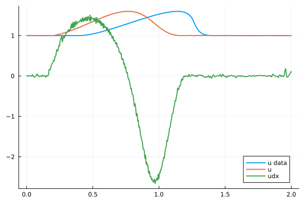
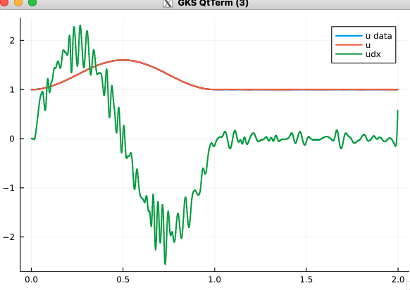
Spatial Derivatives
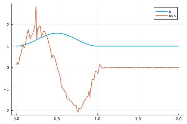
- Spatial derivative \(\dfrac{d}{dx}NN(x)\) are very noisy even when they are computed exactly with forward mode autodiff.
- This is because the function \(u = NN(x)\) has tiny but sharp perturbations all over the place.
Next Steps
- Lots of noise likely due to my choice of activation function (\(elu, \sin\)). Only \(\sin\) should give smooth derivatives.
- Plan is to retrain neural network with only \(\sin\) activation and potentially do gradient supervision.
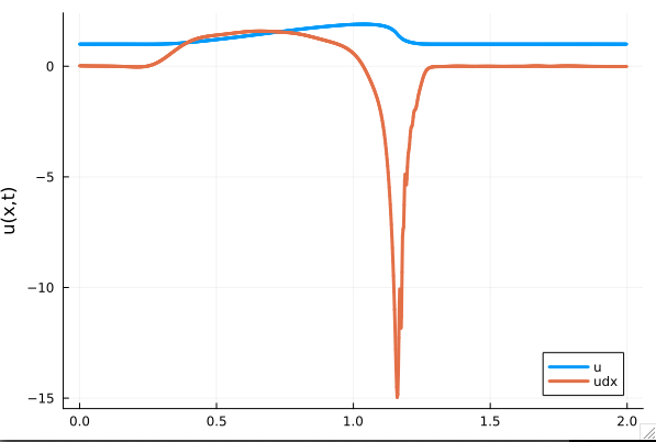
Time-evolution plots
- Solution moving from left to right in time. Performs well initially but distorts due to noisy spatial derivatives.
- When noise is smoothened un-physically, the perturbations reduce in magnitude.
Updates 11/20/23
Topic: Learned latent space with auto-encoders, equation-based time-evolution
Title: Making Nonlinear Model-Order Reduction robust and cheap
Challenges
- Large training cost, large online solve cost
- Robustness of methods
- Changing latent space requires expensive re-training
Possible new contributions
- Speed up training time for SOTA models (few hrs --> few minutes)
- Iteratively improve latent space with sequential model training
- Demonstrate method on large problem with complex physics
Updates from this week
- High-order AD: implemented finite diff, FWD mode AD for spatial derivatives
- Time evolution: implemented Euler FWD/BWD with adaptive time-stepper
- Results are mixed: the methodology works but solution distorts easily
- Reason being that spatial derivatives like \(\frac{d}{dx}\texttt{NN(x)}\) are very noisy
- I know that because errors go down when I smoothen derivatives
- Next step: retrain neural network to ensure smoother derivatives
Plan
- Data Generation (1 day)
- 1D Burgers problem, \(\mathit{Re}=10k\) [done]
- 2D Burgers problem, \(\mathit{Re}=10k\)
- Model Implementation
- Latent space (2 week)
- Encoder free implicit model [done]
- Training strategy, test on many datasets
-
Time evolution (4 week)
- Nonlinear optimizers [done]
- Higher order auto-diff [done]
- Time-evolution schemes [WIP]
- Hyper reduction
- Latent space (2 week)
- Numerical Experiments
- 1D/2D Burgers problem
- 2D Advection equation
- Traveling shock problem with adaptive meshing
Spatial Derivatives
- Spatial derivative \(\dfrac{d}{dx}NN(x)\) are very noisy even when they are computed exactly with forward mode autodiff.
- This is because the function \(u = NN(x)\) has tiny but sharp perturbations all over the place.
Next Steps
- Lots of noise likely due to my choice of activation function (\(elu, \sin\)). Only \(\sin\) should give smooth derivatives.
- Plan is to retrain neural network with only \(\sin\) activation and potentially do gradient supervision.
Time-evolution plots
- Solution moving from left to right in time. Performs well initially but distorts due to noisy spatial derivatives.
- When noise is smoothened un-physically, the perturbations reduce in magnitude.
Updates 11/28/23
Topic: Learned latent space with auto-encoders, equation-based time-evolution
Title: Making Nonlinear Model-Order Reduction robust and cheap
Challenges
- Large training cost, large online solve cost
- Robustness of methods
- Changing latent space requires expensive re-training
Possible new contributions
- Speed up training time for SOTA models (few hrs --> few minutes)
- Iteratively improve latent space with sequential model training
- Demonstrate method on large problem with complex physics
Updates from this week
- Higher order AD, time evolution scheme working.
- Problem: spatial derivatives like \(\dfrac{d}{dx}\texttt{NN(x)}\) are very noisy
- Attempted many architectures, but noise persists
- Literature doesn't say much about it
- This week: do training with gradient supervision to ensure smooth derivatives
- Time off for winter break: planning on leaving Pittsburgh on Fri (12/8).
- Start organizing paper
Plan
- Data Generation (1 day)
- 1D Burgers problem, \(\mathit{Re}=10k\) [done]
- 2D Burgers problem, \(\mathit{Re}=10k\)
- Model Implementation
- Latent space (2 week)
- Encoder free implicit model [done]
- Training strategy, test on many datasets
-
Time evolution (4 week) (+2 weeks)
- Nonlinear optimizers [done]
- Higher order auto-diff [done]
- Time-evolution schemes [WIP]
- Hyper reduction
- Latent space (2 week)
- Numerical Experiments
- 1D/2D Burgers problem
- 2D Advection equation
- Traveling shock problem with adaptive meshing
Updates 12/01/23
Topic: Learned latent space with auto-encoders, equation-based time-evolution
Title: Making Nonlinear Model-Order Reduction robust and cheap
Challenges
- Large training cost, large online solve cost, method robustness
- Changing latent space requires expensive re-training
Possible new contributions
- Speed up training time for SOTA models (few hrs --> few minutes)
- Iteratively improve latent space with sequential model training (boosting)
- Demonstrate method on large problem with complex physics
- Solve the noisy gradients problem
Updates from this week
- Problem: noisy spatial derivatives \(\frac{d}{dx}\texttt{NN(x)}\)
- All surveyed papers sidestep this with inaccurate finite-difference methods
- L2-regularization, over-paramterization help. Consider gradient supervision?
- Continue debugging time-evolution: compare with other paper codes; move to a problem where exact gradients are available; implement Galerkin, Petrov Galerkin projections in time-stepper.
- start organizing paper
Plan
- Data Generation (1 day)
- 1D Burgers problem, \(\mathit{Re}=10k\) [done]
- 2D Burgers problem, \(\mathit{Re}=10k\)
- Model Implementation
- Latent space (2 week)
- Encoder free implicit model [done]
- Training strategy, test on many datasets
-
Time evolution (4 week) (+2 weeks)
- Nonlinear optimizers [done]
- Higher order auto-diff [done]
- Time-evolution schemes [WIP]
- Hyper reduction
- Latent space (2 week)
- Numerical Experiments
- 1D/2D Burgers problem
- 2D Advection equation
- Traveling shock problem with adaptive meshing
Regularization, overparameterization reduces noise in derivatives
With L2-Reguarization, \(\lambda=1\)
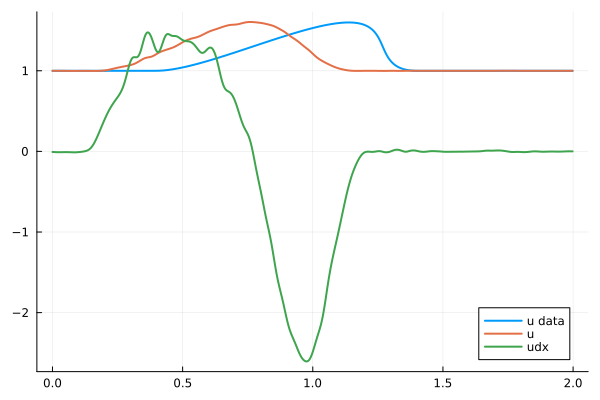
No regularization
Hidden layer width 32
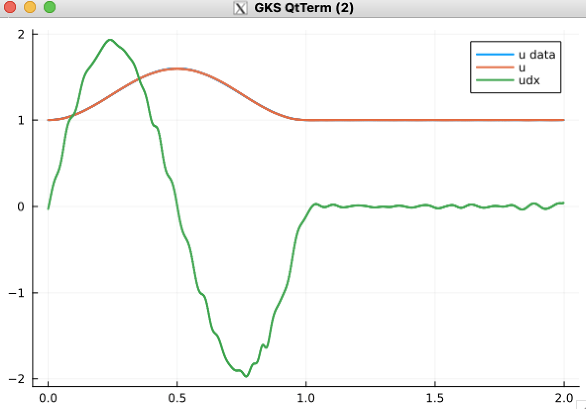
Hidden layer width 256
Updates 12/04/23
Topic: Learned latent space with auto-encoders, equation-based time-evolution
Title: Making Nonlinear Model-Order Reduction robust and cheap
Challenges
- Large training cost, large online solve cost, method robustness
- Changing latent space requires expensive re-training
Possible new contributions
- Speed up training time for SOTA models (few hrs --> few minutes)
Iteratively improve latent space with sequential model training (boosting)- Demonstrate method on large problem with complex physics
- Solve the noisy gradients problem
- Study on density of training samples
Updates from this week
- Problem: noisy spatial derivatives \(\frac{d}{dx}\texttt{NN(x)}\)
- All surveyed papers sidestep this with inaccurate finite-difference methods
- Fixed with L2-regularization, over-paramterization
- Implemented Galerkin, Petrov Galerkin projections in time-stepper
- Next steps: prepare for 2D experiment, start organizing paper
Plan
- Data Generation (1 day)
- 1D Burgers problem, \(\mathit{Re}=10k\) [done]
- 2D Burgers problem, \(\mathit{Re}=10k\)
- Model Implementation
- Latent space (2 week)
- Encoder free implicit model [done]
- Training strategy, test on many datasets
-
Time evolution (4 week) (+2 weeks)
- Nonlinear optimizers [done]
- Higher order auto-diff [done]
- Time-evolution schemes (Galerkin, LSPG)
- Hyper reduction
- Latent space (2 week)
- Numerical Experiments
- 1D/2D Burgers problem
- 2D Advection equation
- Traveling shock problem with adaptive meshing
Test pipeline works on Advection Equation
Solution, first derivative
Predicted Solution matches with data
\( \partial_t u + c\cdot\partial_x u = 0\)
- Using exact Forward Model automatic differentiation
- First order forward Euler time-integration
- Least Squares Petrov Galerkin (nonlinear projection method): MSE: \(10^{-5} ,\, 0.3\%\) relative error
- \( \tilde{u}^{n+1} = \argmin_{\tilde{u}^{n+1}} \|\dfrac{g(\tilde{u}^{n+1})-g(\tilde{u}^{n})}{\Delta t} - f(x, t, g(\tilde{u}^{n+1}) \|_2^2\)
- Time taken: \(0.1s\) without hyper-reduction (comparable highly optimized original solve)
- POD Galerkin (linear projection method): MSE: \(5\cdot10^{-7} ,\, 0.07\%\) relative error
- \( \mathbf{J_g} \cdot\dfrac{\tilde{u}^{n+1}-\tilde{u}^{n}}{\Delta t} = f(x, t, g(\tilde{u}^{n}))\)
- Time taken: \(3s\) without hyper-reduciton.
Advection Equation
- No shocks
- Smaller case, faster training
- Exact solution available for debugging
Back to the Burgers problem
Predicted Solution matches with data

- Using exact Forward Model automatic differentiation
- Galerkin, LSPG returning MSE: \(10^{-5}, \,\, 0.3\%\) relative error
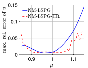
- Accuracy better than literature
Kim, Choi, Widemann, Zhodi, 2020

Problems
- Requires fixed grid, large autoencoder models
- Noisy spatial derivatives \(\frac{d}{dx}\texttt{NN(x)}\)
- All surveyed papers sidestep this with inaccurate finite-difference methods
- \(\Delta x\) becomes another hyper-parameter
- Some even maintain a background mesh
- Solution: Employing larger models with L2-regularization. What else?
Current problems and possible new contributions
Contributions
- Demonstrate method on large problem with complex physics and adaptive meshing
-
Solve the noisy gradients problem
- L2-regularization
- Gradients become less noisy with over-parameterization
- Comparison bw Galerkin, Least Square Petrov Galerkin
- Study on density of sampling (in time, parameter space) in training set
- Speed up training time for SOTA models (few hrs --> few minutes)
- Study density of training samples in time, parameter space
- Study on latent space size
- Compare classes of models (POD, conv. AE, SIREN, partition of unity models as a case of domain decomposition methods)
- Other ideas:
- Think about variational inference (especially at shocks)
- Iteratively improve latent space with sequential model training (boosting)
Updates 12/18/23
Topic: Learned latent space with auto-encoders, equation-based time-evolution
Title: Making Nonlinear Model-Order Reduction robust and cheap
Possible new contributions
- Speed up training time for SOTA models (few hrs --> few minutes)
Iteratively improve latent space with sequential model training (boosting)- Learn ROMs from simulations with adaptive grids
- Solve the noisy spatial derivative problem
- Demonstrate method on large problem with complex physics
Updates from this week
- Implemented Galerkin, Petrov Galerkin projections in time-stepper
- Generate data for 1D KS problem
- In progress:
- Implementing high order time stepper
- Kuramuto-Sivashinsky case setup
- Paper intro, contributions, related work
- Blockers:
- Data generation
Plan
- Data Generation (1 day)
- 1D Burgers problem, \(\mathit{Re}=10k\) [done]
- 2D Burgers problem, \(\mathit{Re}=10k\)
- Model Implementation
- Latent space (2 week)
- Encoder free implicit model [done]
- Training strategy, test on many datasets
-
Time evolution (4 week)
- Nonlinear solvers [done]
- Higher order auto-diff [done]
- Time-evolution schemes (Galerkin, LSPG)
Hyper-reduction
- Latent space (2 week)
- Numerical Experiments
- 1D Advection, 1D Burgers [done]
- 2D Advection, 2D Burgers
- 1D/2D Kuramoto-Sivashinsky
1D Kuramoto-Sivashinsky equation in on \([0,10\pi)\) periodic
Challenge:
- No way to enforce periodicity constraint on ROMs (classical or ML)
- For existing ML-ROM, this would require special treatment at boundary.
Updates 01/08/24
Topic: Learned latent space with auto-encoders, equation-based time-evolution
Title: Making Nonlinear Model-Order Reduction robust and cheap
Possible new contributions
- Speed up training time for SOTA models (few hrs --> few minutes)
- Learn ROMs from simulations with adaptive grids
- Solve the noisy spatial derivative problem
- Demonstrate method on large problem with complex physics
Updates from this week
- Paper writing: contributions, problem setup, methodology
- Experiments:
- Assess effect of regularization in reducing gradient noise
- Kuramoto-Sivashinsky equation
- High order time-steppers
- Blockers: Extreme lag because GPU machines are far away
Plan
- Data Generation (1 day)
- 1D Burgers problem, \(\mathit{Re}=10k\) [done]
- 2D Burgers problem, \(\mathit{Re}=10k\)
- Model Implementation
- Latent space (2 week)
- Encoder free implicit model [done]
- Training strategy, test on many datasets
-
Time evolution (4 week)
- Nonlinear solvers [done]
- Higher order auto-diff [done]
- Time-evolution schemes (Galerkin, LSPG)
Hyper-reduction
- Latent space (2 week)
- Numerical Experiments
- 1D Advection, 1D Burgers [done]
- 2D Advection, 2D Burgers
- 1D/2D Kuramoto-Sivashinsky
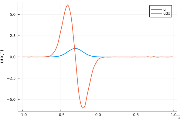
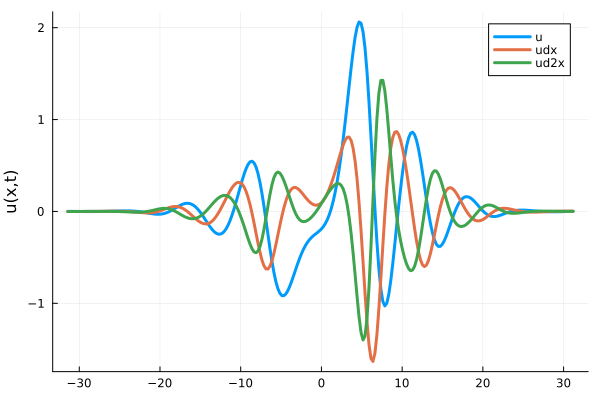
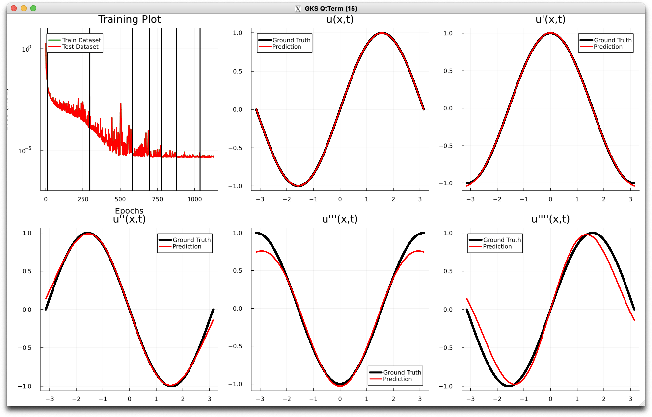
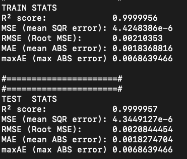
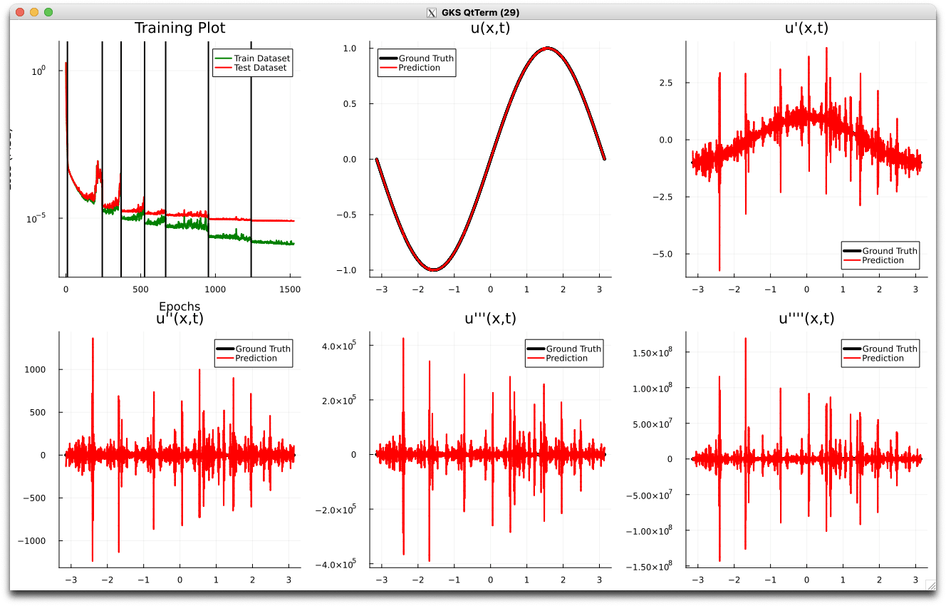
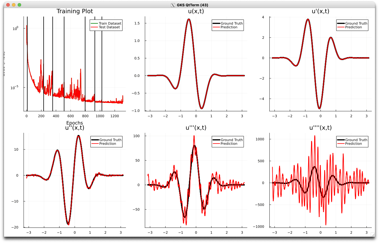
1D Kuramoto-Sivashinsky equation
- Learning spatial representation
- Noisy gradient problem is fully eliminated.
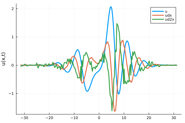
- All derivatives up to fourth order are completely smooth. MSE~\(10^{-6}\)
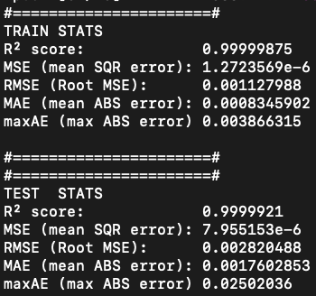
- Time-evolution
- Problem extremely stiff: PDE solver takes ~100k steps to simulate
- Dynamics are not being captured due to the need for extremely small time-steps.
- I am experimenting with simpler problems
\(\lambda = 0 \) (no regularization)
\(\lambda = 0.5\)
1D Kuramoto-Sivashinsky equation
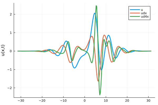
- Fourth derivative (green line) is completely smooth
Updates 01/16/24
Topic: Learned latent space with auto-encoders, equation-based time-evolution
Title: Making Nonlinear Model-Order Reduction robust and cheap
Possible new contributions
- Speed up training time for SOTA models (few hrs --> few minutes)
- Learn ROMs from simulations with adaptive grids
- Solve the noisy spatial derivative problem
- Demonstrate method on large problem with complex physics
Updates from this week
- Paper writing: Latent space,
- Experiments:
- Assess effect of regularization in reducing gradient noise
- Fix Kuramoto-Sivashinsky data. Present simulation too stiff.
- Generated data for 2D advection problem
- Literature study on noise in spatial derivatives
Plan
- Data Generation (1 day)
- 1D Burgers problem, \(\mathit{Re}=10k\) [done]
- 2D Burgers problem, \(\mathit{Re}=10k\)
- Model Implementation
- Latent space (2 week)
- Encoder free implicit model [done]
- Training strategy, test on many datasets
-
Time evolution (4 week)
- Nonlinear solvers [done]
- Higher order auto-diff [done]
- Time-evolution schemes (Galerkin, LSPG)
Hyper-reduction
- Latent space (2 week)
- Numerical Experiments
- 1D Advection, 1D Burgers [done]
- 2D Advection, 2D Burgers
- 1D Kuramoto-Sivashinsky
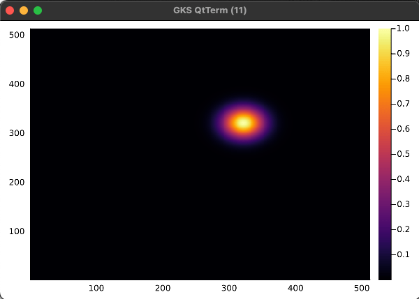
2D Advection Problem
- Demonstrate the ability of our method to work with
- Complex geometry
- Unstructured grid
- Adaptive mesh
- Plan
- Simulate a gaussian traveling in a circle over a large domain
- After simulation is done, clip the domain to simulate complex geometry
- Subsample points away from the gaussian to simulate adaptive mesh
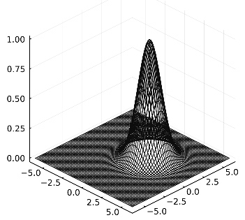
Initial condition
How effective are we at removing noise from \(\partial_x NN(x)\)?
Ours
Baseline
How effective are we at removing noise from \(\partial_x NN(x)\)?
- Obviously, noise worsens with the condition number of the problem.
- Nevertheless, we are able to control noise, as well as capture shocks, for the problems we are concerned with.
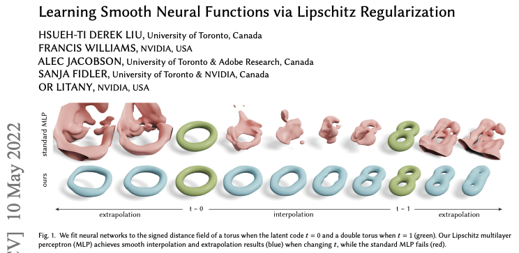
How effective are we at removing noise from \(\partial_x NN(x)\)?
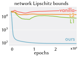
- There is very little literature on this topic.
- This paper is concerned with smoothly interpolating b/w shapes
- They are able to make networks smooth by adding the Lipschitz constant of each layer to the loss function.
- This is similar to our approach, i.e. penalizing L2 norm of decoder weights
- However, they claim to have better results (of course in a different field)
- Other approaches that can help are:
- Turning the autodecoder into a "variational autodecoder" by regularizing over learned latent vectors by adding
\( \dfrac{1}{\sigma^2} ||\tilde{u}||_2 \) to loss. This would make \(\tilde{u}\) more compact and likely reduce the number of time-samples needed. - Lipschitz constant of \(x \to NN(x) \) worsens with the number of layers in NN. Tweak architecture by inserting \(x\) in later layers
- Turning the autodecoder into a "variational autodecoder" by regularizing over learned latent vectors by adding
Updates 01/19/24
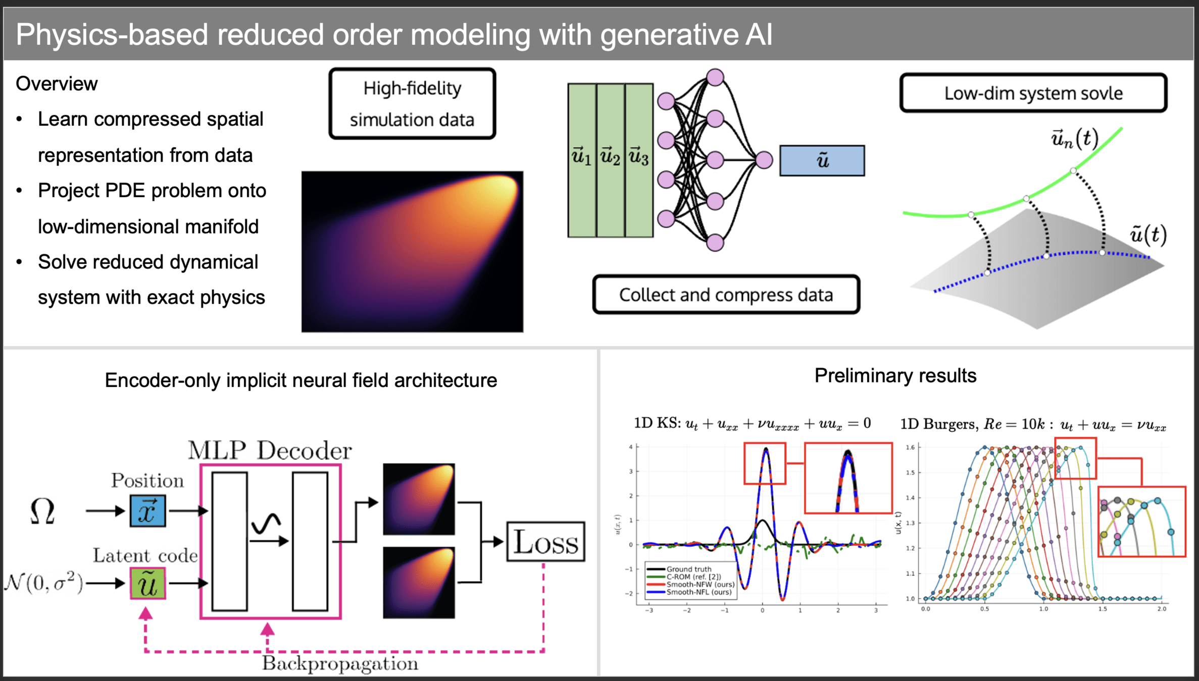
Nonlinear Manifold Reduced Order Modeling with Neural Fields
Existing methods
- PCA based methods don't work well for advection dominated problems
- Autoencoder based methods have large training/evaluation cost
- Implicit Neural Representations suffer from non-smooth interpolations, and either learn dynamics from data, or use inaccurate spatial derivatives
New Contributions
- Solve the problem with non-smooth interpolation with INRs
- A smooth interpolation preserves higher order derivatives of the target function, which we compute exactly with AD
- We implement the pipeline in Julia which allows for highly efficient GPU implementation of forward mode automatic differentiation
Progress
- Experiments on performance of regularization
- Implemented high order time-steppers (RK-2, RK-4)
- Getting a very good performance boost.
- My un-optimized ROM is now faster than FOM code for both 1D cases
- Next Week: 2D advection, Methods section
Writing Plan
- Introduction
- Background
- existing methods [in progress]
- problem formulation [done]
- Methods [finish 1/23]
- Manifold learning
- encoder free [in progress]
- smoothing
- Latent space dynamics [finish 1/23]
- LSPG, Petrov Galerkin [in progress]
- Manifold learning
- Experiments [finish 1/25]
- 1D viscous Burgers [done]
- 1D advection [done]
- 1D Kuramoto-Sivashinsky
- 2D advection
- 2D Burgers
Updates 01/19/24
Nonlinear Manifold Reduced Order Modeling with Neural Fields
Existing methods
- PCA based methods don't work well for advection dominated problems
- Autoencoder based methods have large training/evaluation cost
- Implicit Neural Representations suffer from non-smooth interpolations, and either learn dynamics from data, or use inaccurate spatial derivatives
New Contributions
- Solve the problem with non-smooth interpolation with INRs
- A smooth interpolation preserves higher order derivatives of the target function, which we compute exactly with AD
- We implement the pipeline in Julia which allows for highly efficient GPU implementation of forward mode automatic differentiation
Progress
- Scale ROM code to 2D, and solve the advection problem
- Implement some regularization techniques
- more smoothing
- need less snapshots to capture dynamics
- Start writing Abstract for WCCM conference
Writing Plan
- Abstract [finish 1/29]
- Introduction
- Background
- existing methods [in progress]
- problem formulation [done]
- Methods [finish 1/3]
- Manifold learning
- encoder free [in progress]
- smoothing
- Latent space dynamics [finish 2/7]
- LSPG, Petrov Galerkin [in progress]
- Multistep timesteppers
- Manifold learning
- Experiments [finish 2/12]
- 1D viscous Burgers [done]
- 1D advection [done]
- 1D Kuramoto-Sivashinsky
- 2D advection [1/25]
- 2D Burgers
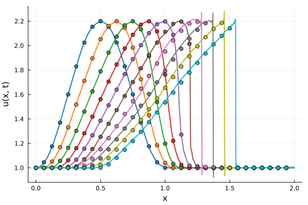
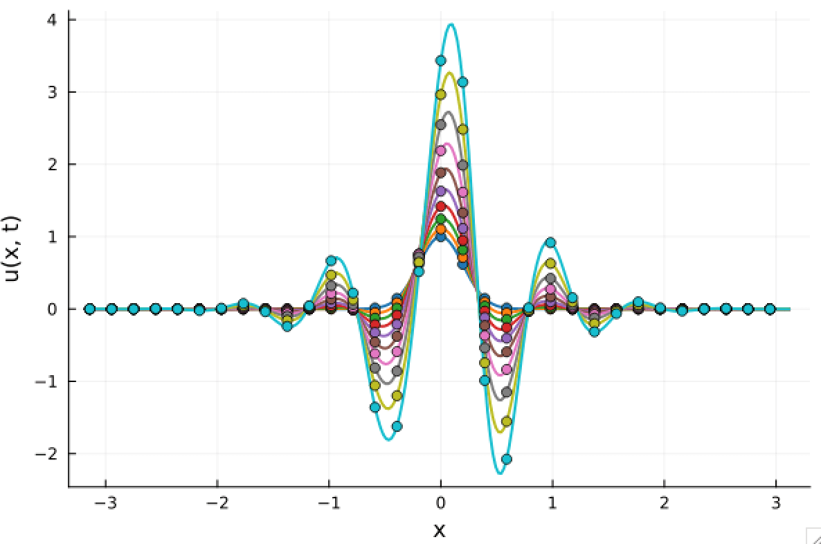
2D Advection Problem
- Traveling shock problem
- Very hard for PCA based ROMs
- Would need 100s of PCA modes
- ML model captures it with only 8 modes
- MSE: \(\approx10^{-9}\)
- Relative error: \( 0.05\%\)
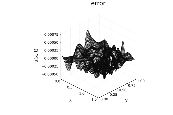
Solution (red), Data (black)
Error at last time-step
Updates 02/01/24
Nonlinear Manifold Reduced Order Modeling with Neural Fields
Existing methods
- PCA based methods don't work well for transport problems
- Autoencoder based methods have large training/evaluation cost
- Implicit Neural Representations (INRs) suffer from non-smooth interpolations, and either learn dynamics from data, or use inaccurate spatial derivatives
New Contributions
- Solve the problem with non-smooth interpolation with INRs
- A smooth interpolation preserves higher order derivatives of the target function, which we compute exactly with AD
- We implement the pipeline in Julia which allows for highly efficient GPU implementation of forward mode automatic differentiation
Progress
- Accepted at WCCM 2024
- Abstract for MechE PhD Symposium
- Implemented smoothness measures
- Paper writing
Writing Plan
- Abstract [finish 1/29]
- Introduction [finish 2/3]
- existing methods [done]
- motivation, contribution [nearly done]
- problem formulation [done]
- Methods [finish 2/5]
- Manifold learning
- encoder free [done]
- smoothing [in progress]
- Latent space dynamics [finish 2/5]
- LSPG, Petrov Galerkin [in progress]
- Multistep timesteppers
- Manifold learning
- Experiments [finish 2/12]
- 1D viscous Burgers
- 1D advection
- 1D Kuramoto-Sivashinsky
- 2D advection
- 2D Burgers
Updates 02/08/24
Nonlinear Manifold Reduced Order Modeling with Neural Fields
Existing methods
- PCA based methods don't work well for transport problems
- Autoencoder based methods have large training/evaluation cost
- Implicit Neural Representations (INRs) suffer from non-smooth interpolations, and either learn dynamics from data, or use inaccurate spatial derivatives
New Contributions
- Solve the problem with non-smooth interpolation with INRs
- A smooth interpolation preserves higher order derivatives of the target function, which we compute exactly with AD
- We implement the pipeline in Julia which allows for highly efficient GPU implementation of forward mode automatic differentiation
Progress
- Gather remaining results
- Implement other models for comparison
- PCA ROM
- Auto-encoder ROM
- Neural field ROM
Writing Plan
- Abstract [done]
- Introduction [done]
- motivation [done]
- lit review [done]
- contributions [done]
-
- Manifold learning
- problem formulation [done]
- encoder free [done]
- smoothing [60%]
- Latent space dynamics [60%]
- LSPG, Petrov Galerkin
- Multi-stage time-steppers
- Manifold learning
- Experiments [finish 2/12]
- 1D / 2D viscous Burgers
- 1D / 2D advection
- 1D Kuramoto-Sivashinsky
Kuramoto-Sivashinsky Equation
- Maximum error: \( 2\%\) (normalized)
- Average error: \(0.4\%\) (normalized)
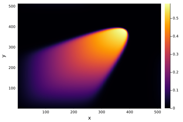
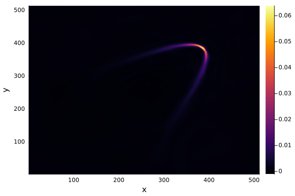
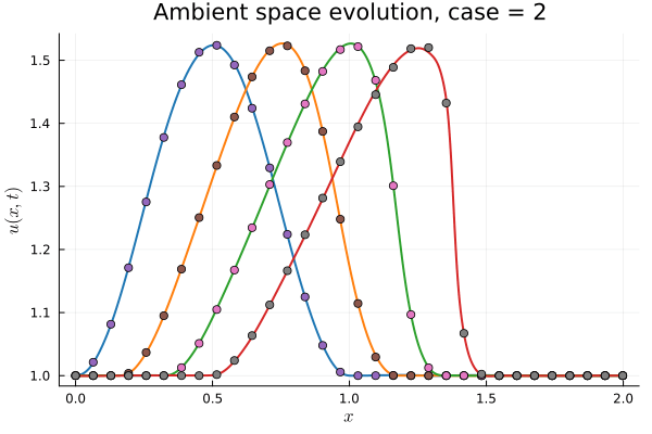
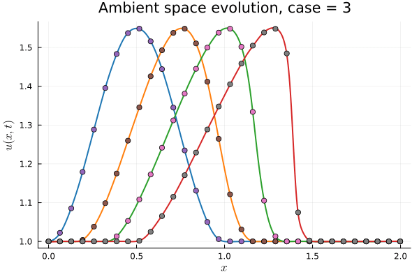
2D Burgers problem
- Reproducing example by Li, et al.
- Reynolds number \(1000\)
- Data generation on \(512 \times 512 \) grid on periodic box domain \([0,1)^2\)
- Training on \(128\times 128\) in progress
Updates 02/16/24
Nonlinear Manifold Reduced Order Modeling with Neural Fields
Existing methods
- PCA based methods don't work well for transport problems
- Autoencoder based methods have large training/evaluation cost
- Implicit Neural Representations (INRs) suffer from non-smooth interpolations, and either learn dynamics from data, or use inaccurate spatial derivatives
New Contributions
- Solve the problem with non-smooth interpolation with INRs
- A smooth interpolation preserves higher order derivatives of the target function, which we compute exactly with AD
- We implement the pipeline in Julia which allows for highly efficient GPU implementation of forward mode automatic differentiation
Progress
- Gathered all results
- Implement other models for comparison
- PCA ROM, Auto-encoder ROM, Neural field ROM
- Experiment Multi-GPU training
Writing Plan
- Abstract [done]
- Introduction [done]
- motivation [done]
- lit review [done]
- contributions [done]
-
- Manifold learning
- problem formulation [done]
- encoder free [done]
- smoothing [60%]
- Latent space dynamics [60%]
- LSPG, Petrov Galerkin
- Multi-stage time-steppers
- Manifold learning
- Experiments [finish 2/12]
- 1D / 2D viscous Burgers
- 1D / 2D advection
- 1D Kuramoto-Sivashinsky
- Write results section
2D Burgers problem
- Reproducing example by Li, et al.
- Reynolds number \(1000\)
- Data generation on \(512 \times 512 \) grid on periodic box domain \([0,1)^2\)
- Training on \(128\times 128\) in progress
- Mean error: \(1\%\)
- Solution at final time-step:
Updates 02/22/24
Nonlinear Manifold Reduced Order Modeling with Neural Fields
Existing methods
- PCA based methods don't work well for transport problems
- Autoencoder based methods have large training/evaluation cost
- Implicit Neural Representations (INRs) suffer from non-smooth interpolations, and either learn dynamics from data, or use inaccurate spatial derivatives
New Contributions
- Solve the problem with non-smooth interpolation with INRs
- A smooth interpolation preserves higher order derivatives of the target function, which we compute exactly with AD
Progress
- paper writing: implementing comparison models from literature
- model training pipeline works
- working on time evolution: implement derivatives on FEM mesh
- making figures for poster
Writing Plan
- Abstract [done]
- Introduction [done]
- motivation [done]
- lit review [done]
- contributions [done]
-
- Manifold learning
- problem formulation [done]
- encoder free [done]
- smoothing [80%]
- Latent space dynamics [60%]
- LSPG, Petrov Galerkin
- Multi-stage time-steppers
- Manifold learning
- Experiments [done]
- 1D / 2D viscous Burgers
- 1D / 2D advection
- 1D Kuramoto-Sivashinsky
- Results []
- Conclutions []
Zhang Group Meeting - 03/01/2024
Nonlinear Manifold Reduced Order Modeling with Neural Fields
Vedant Puri
Curse of dimensionality in approximation theory
| Orthogonal Functions | Deep Neural Networks |
|---|---|
|
|
|
Curse of dimensionality
Dimension independent
Model size scales only with the complexity of the signal.
Landscape of ML for PDEs
Mesh-based
PDE-Based
Neural Ansatz
Data-driven
FEM, FVM, IGA, Spectral
Fourier Neural Operator
Implicit Neural Representations
DeepONet
Physics Informed NNs
Convolution NNs
Graph NNs
Adapted from Núñez, CEMRACS 2023
Neural ODEs
Universal Diff Eq
Reduced Order Modeling
Updates 02/22/24
Nonlinear Manifold Reduced Order Modeling with Neural Fields
Existing methods
- PCA based methods don't work well for transport problems
- Autoencoder based methods have large training/evaluation cost
- Implicit Neural Representations (INRs) suffer from non-smooth interpolations, and either learn dynamics from data, or use inaccurate spatial derivatives
New Contributions
- Solve the problem with non-smooth interpolation with INRs
- A smooth interpolation preserves higher order derivatives of the target function, which we compute exactly with AD
Progress this week
- Results are favorable for linear equations, unfavorable for nonlinear eqns
- Tracking the source of the error
Writing Plan
- Abstract [done]
- Introduction [done]
- motivation
- lit review
- contributions [done]
-
- Manifold learning
- problem formulation
- encoder free
- smoothing
- Latent space dynamics [done]
- Galerkin projection
- Multi-stage time-steppers
- Manifold learning
- Experiments [done]
- 1D / 2D viscous Burgers
- 1D / 2D advection
- 1D Kuramoto-Sivashinsky
- Results []
- Conclutions []
Updates 03/19/24
Nonlinear Manifold Reduced Order Modeling with Neural Fields
Existing methods
- PCA based methods don't work well for transport problems
- Autoencoder based methods have large training/evaluation cost
- Implicit Neural Representations (INRs) suffer from non-smooth interpolations, and either learn dynamics from data, or use inaccurate spatial derivatives
New Contributions
- Solve the problem with non-smooth interpolation with INRs
- A smooth interpolation preserves higher order derivatives of the target function, which we compute exactly with AD
Progress this week
- Made some workflow figures for professor Kara.
- Results are favorable for linear equations, unfavorable for nonlinear eqns
- Tracking the source of the error
Writing Plan
- Abstract [done]
- Introduction [done]
- motivation
- lit review
- contributions [done]
-
- Manifold learning
- problem formulation
- encoder free
- smoothing
- Latent space dynamics [done]
- Galerkin projection
- Multi-stage time-steppers
- Manifold learning
- Experiments [done]
- 1D / 2D viscous Burgers
- 1D / 2D advection
- 1D Kuramoto-Sivashinsky
- Results []
- Conclutions []
1D Advection

Smooth Neural Field Weight Regularization
Smooth Neural Field Lipschitz Regularization
1D KS
Smooth Neural Field Weight Regularization
Smooth Neural Field Lipschitz Regularization


1D Burgers: Smooth Neural Field Weight Regularization


1D Burgers: Smooth Neural Field Lipschitz Regularization
Workflow slide for Professor Kara
Updates 03/21/24
Nonlinear Manifold Reduced Order Modeling with Neural Fields
Existing methods
- PCA based methods don't work well for transport problems
- Autoencoder based methods have large training/evaluation cost
- Implicit Neural Representations (INRs) suffer from non-smooth interpolations, and either learn dynamics from data, or use inaccurate spatial derivatives
New Contributions
- Solve the problem with non-smooth interpolation with INRs
- A smooth interpolation preserves higher order derivatives of the target function, which we compute exactly with AD
Progress this week
- Identified a source of discrepancy in results
- Implementing the fix.
Writing Plan
- Abstract [done]
- Introduction [done]
- motivation
- lit review
- contributions [done]
-
- Manifold learning
- problem formulation
- encoder free
- smoothing
- Latent space dynamics [done]
- Galerkin projection
- Multi-stage time-steppers
- Manifold learning
- Experiments [done]
- 1D / 2D viscous Burgers
- 1D / 2D advection
- 1D Kuramoto-Sivashinsky
- Results []
- Conclutions []
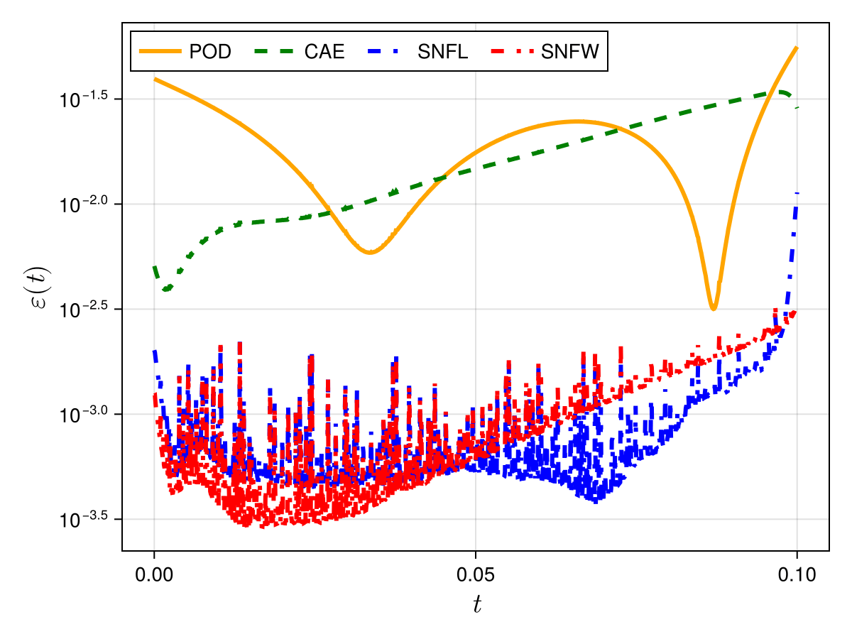
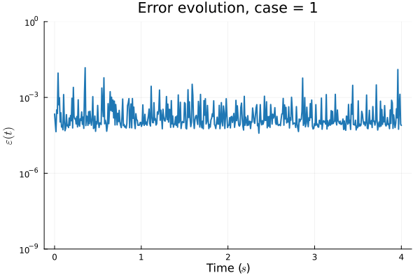
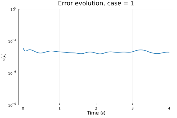
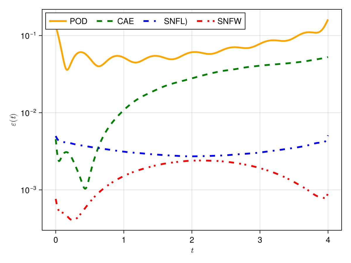
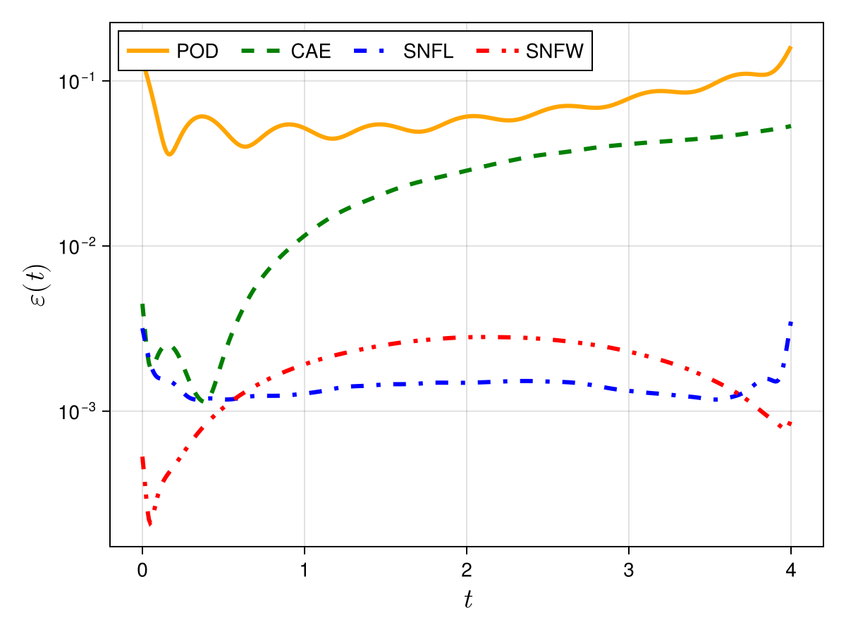
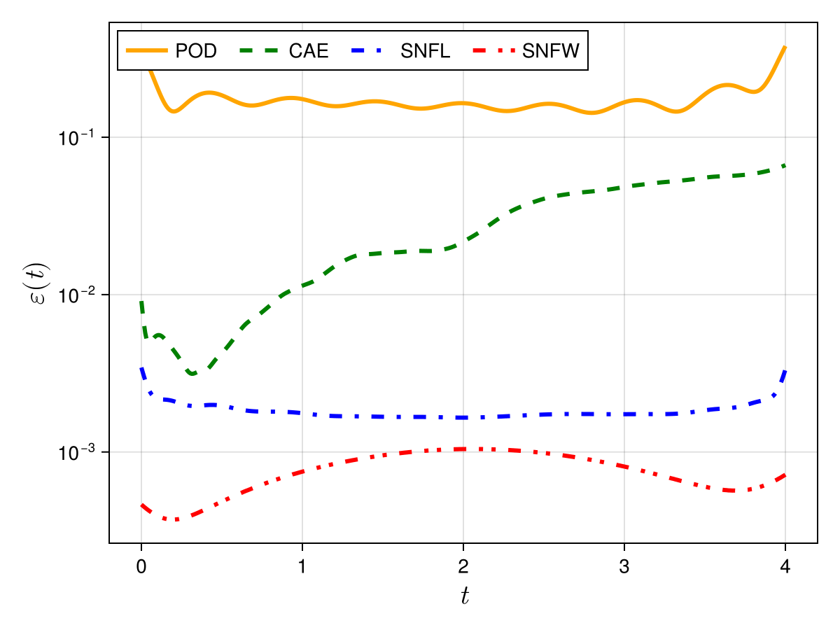
1D Advection: Deep Convolutional Autoencoder (Lee, Carlberg 2021)

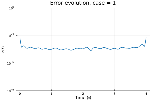
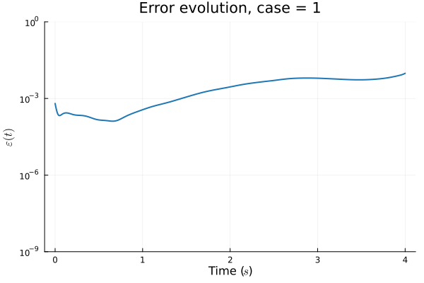
Training error
Evolution error

1D Advection: Smooth Neural Field Weight Regularization (ours)
Training error
Evolution error
1D Advection: Smooth Neural Field Lipschitz Regularization (ours)
Training error
Evolution error
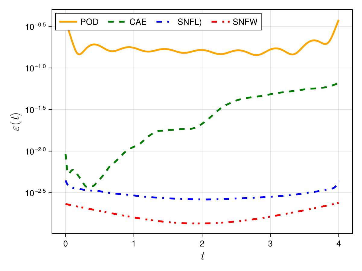
1D KS: Deep Convolutional Autoencoder (Lee, Carlberg 2021)
Training error
Evolution error
1D KS: Smooth Neural Field Weight Regularization (ours)
Training error
Evolution error

1D KS: Smooth Neural Field Lipschitz Regularization (ours)
Training error
Evolution error
The fix
Problem:
- In Deep CAE (Lee, Carlberg 2021), the latent space coordinates are along a low-dimensional manifold.
- Our latent space representations are irregular, disconnected.
Fix:
- Flatten latent space representations to lie along a low-dimensional space.
- Introduce a hyper-network to predict latent coordinates as a function of time.
(Cho et al. 2023)
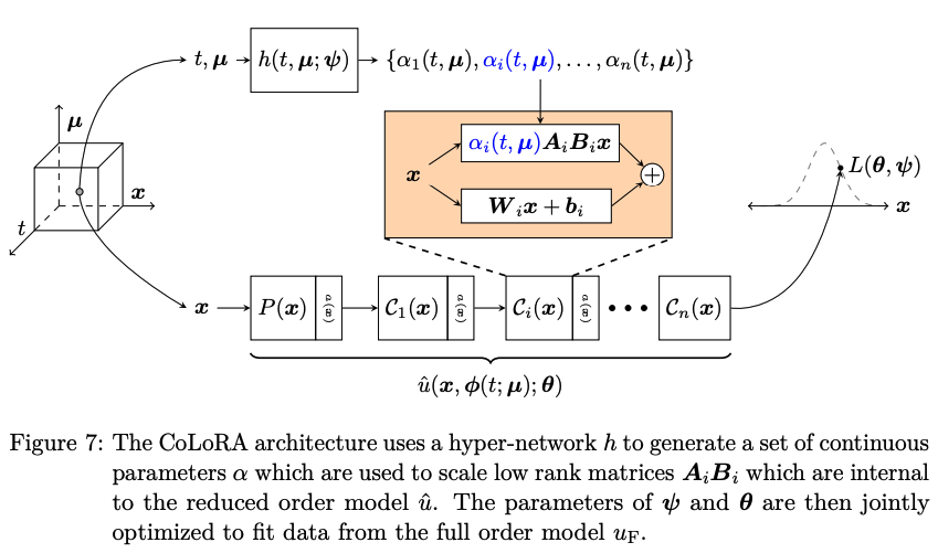
(Berman et al. 2024)
Updates 03/22/24
Nonlinear Manifold Reduced Order Modeling with Neural Fields
Existing methods
- PCA based methods don't work well for transport problems
- Autoencoder based methods have large training/evaluation cost
- Implicit Neural Representations (INRs) suffer from non-smooth interpolations, and either learn dynamics from data, or use inaccurate spatial derivatives
New Contributions
- Solve the problem with non-smooth interpolation with INRs
- A smooth interpolation preserves higher order derivatives of the target function, which we compute exactly with AD
Progress this week
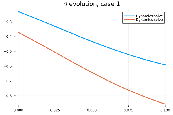
- Problem: Latent coordinates not are disjoint and irregular. Dynamics solve can't traverse latent space.
Writing Plan
- Abstract [done]
- Introduction [done]
- motivation
- lit review
- contributions [done]
-
- Manifold learning
- problem formulation
- encoder free
- smoothing
- Latent space dynamics [done]
- Galerkin projection
- Multi-stage time-steppers
- Manifold learning
- Experiments [done]
- 1D / 2D viscous Burgers
- 1D / 2D advection
- 1D Kuramoto-Sivashinsky
- Results []
- Conclutions []
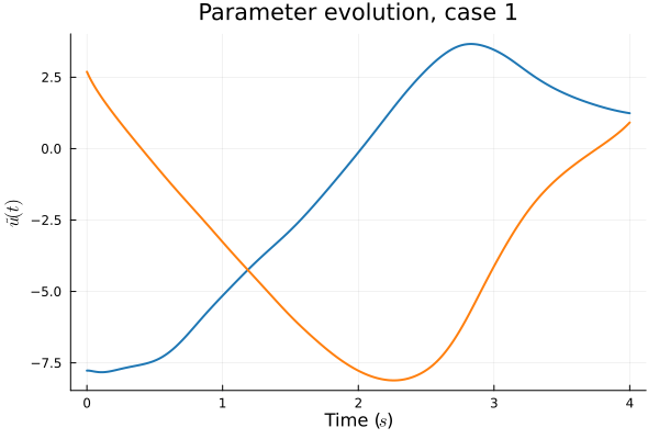
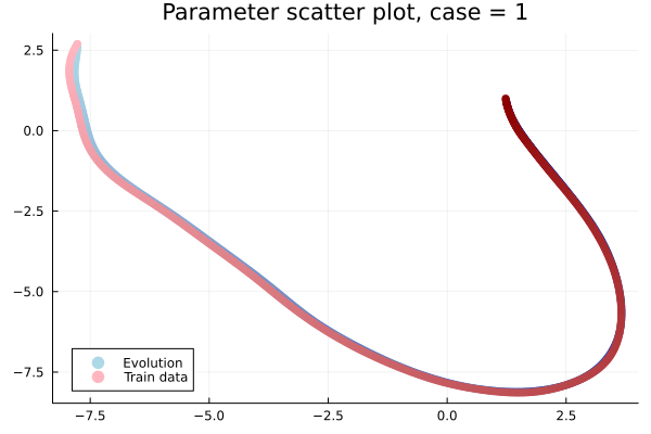
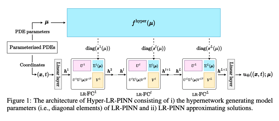
Architecutre
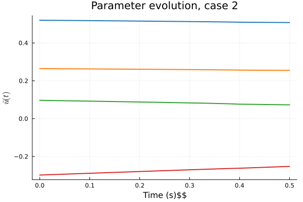
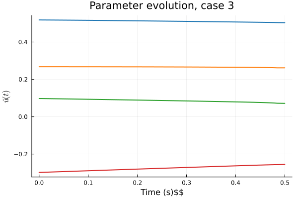
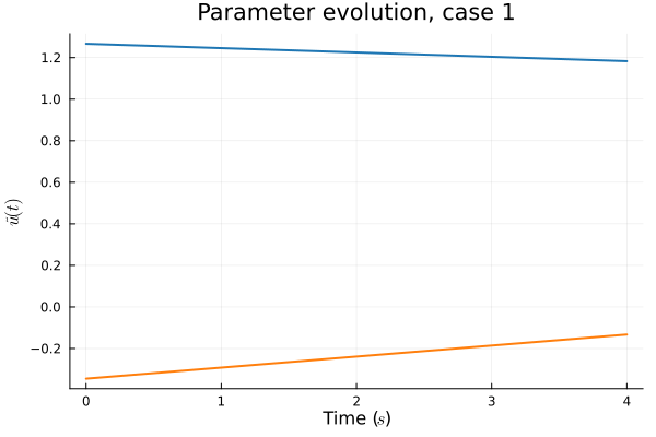
Parameterized PDE Problem (\( \vec{x}, t, \vec{\mu} \))
\( t, \vec{\mu}\)
Hyper Network
\( \vec{x}\)
Decoder Network
\(\tilde{u}\)
\(\vec{u}(\vec{x}, t; \vec{\mu})\)
Physical coordinates
Time, paramters
Latent coordinates
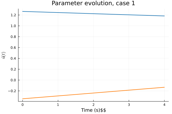
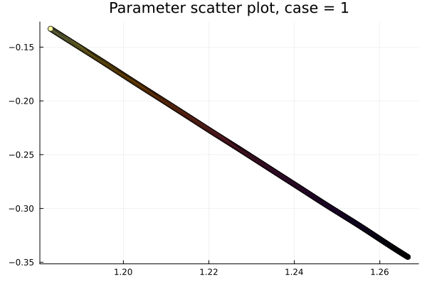
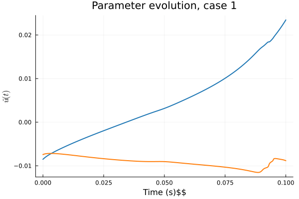
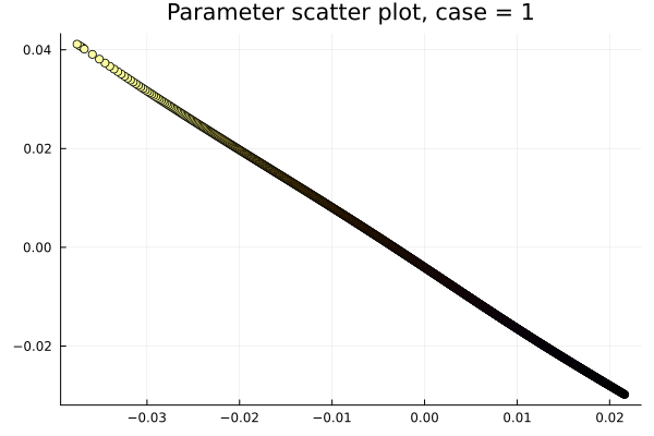
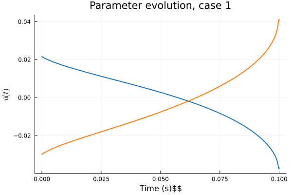
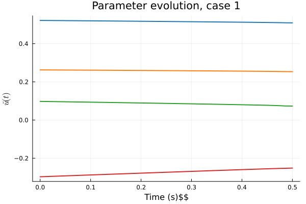
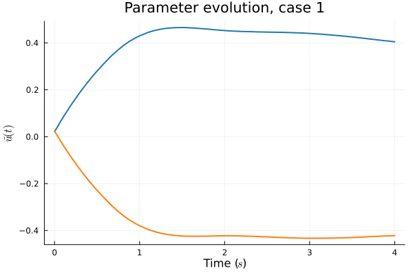
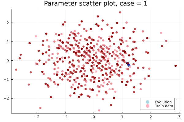
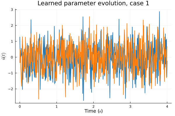
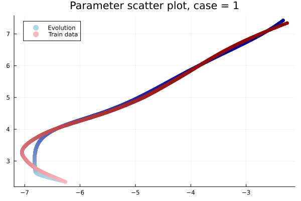
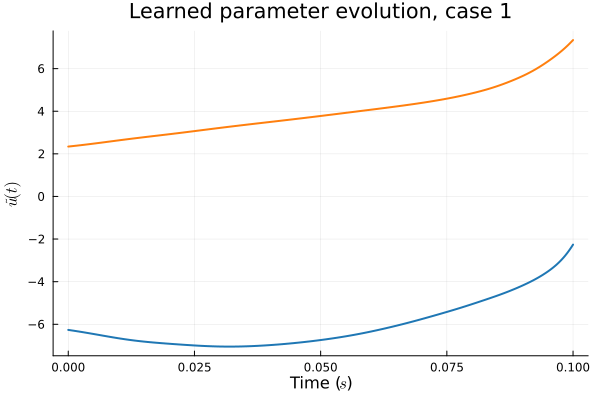
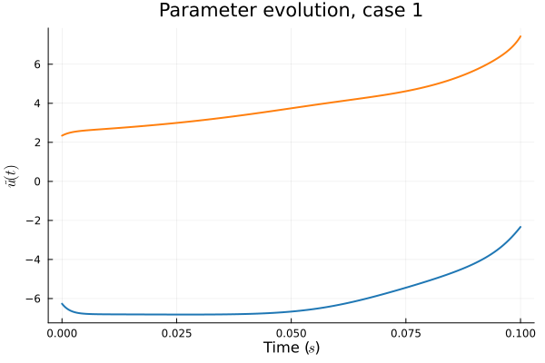
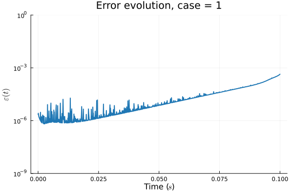
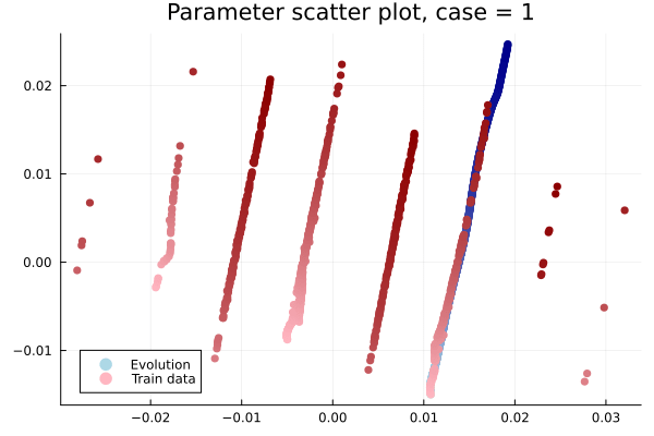
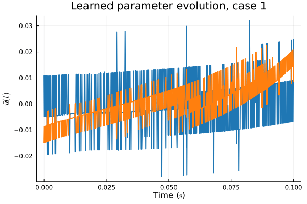
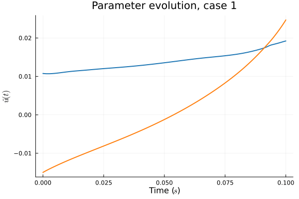
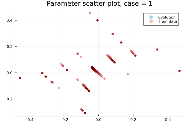
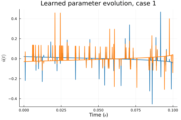
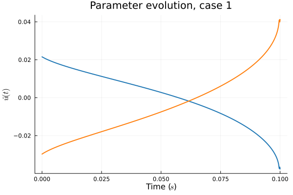
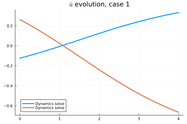
- Problem: Latent coordinates not are disjoint and irregular. Dynamics solve can't traverse latent space.
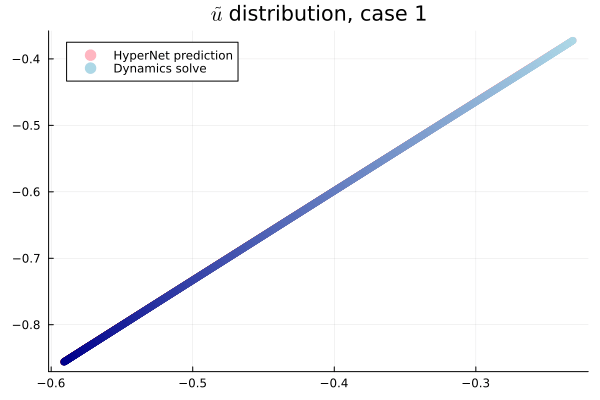
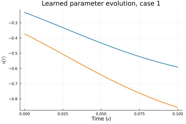
- Fix: Learn a secondary network that predicts latent coordinates. This forces the latent coordinates to lie along a continuous curve.
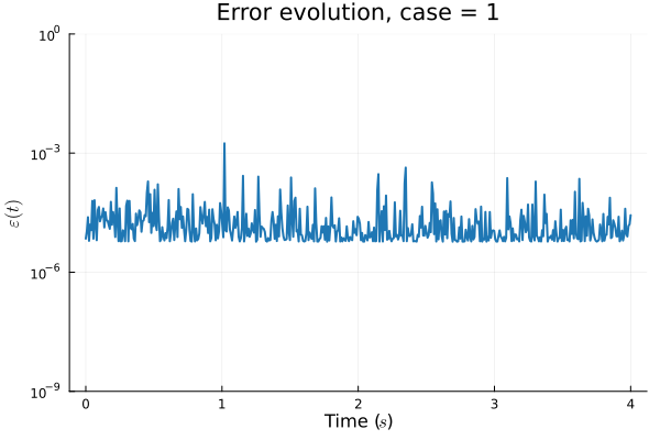
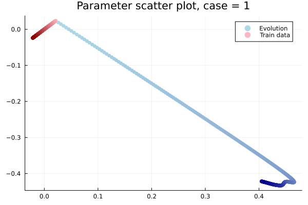
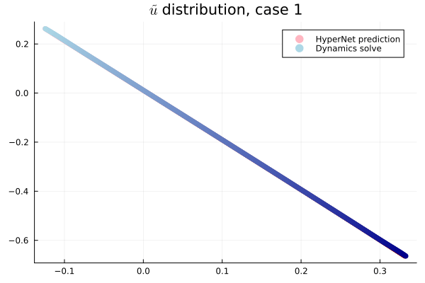
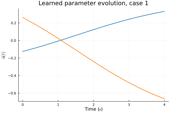
Notes
- Training: Models train in 5x fewer epochs, and converge to a lower loss value.
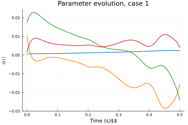
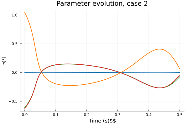
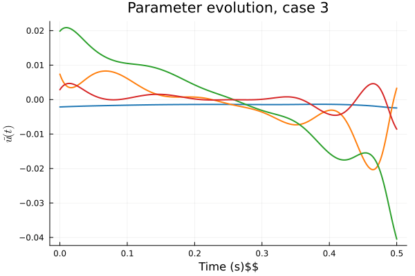
- HyperNet: small, shallow network (~100 params).
- Latent space coordinates, i.e. output of HyperNet, lie along a smooth continuous curve.
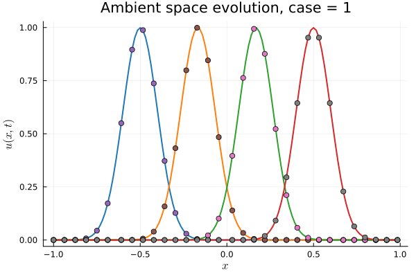
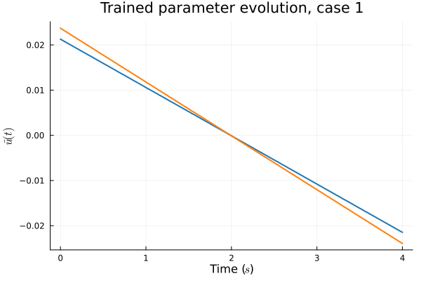
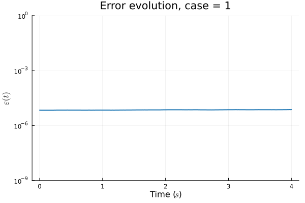
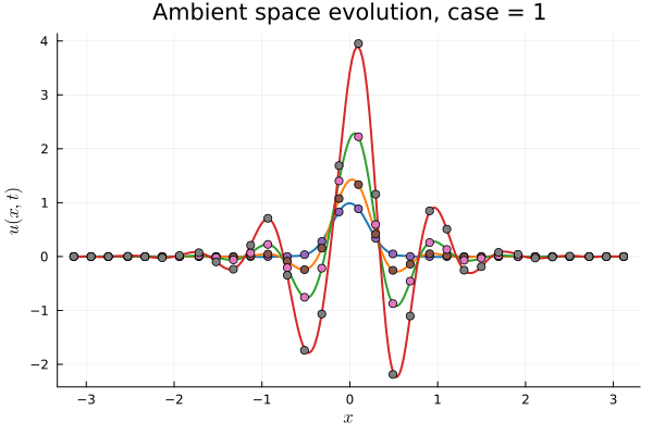
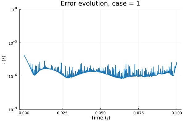
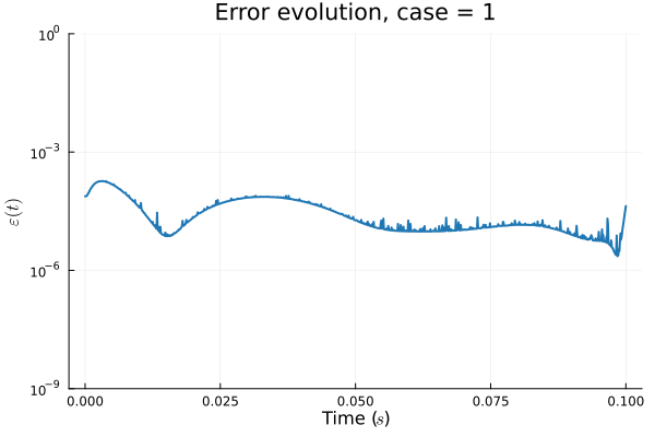
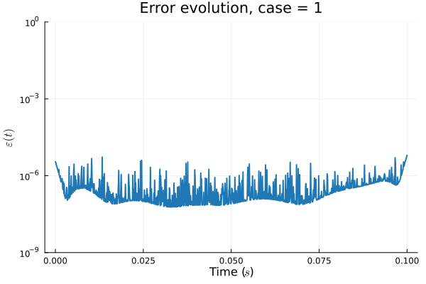
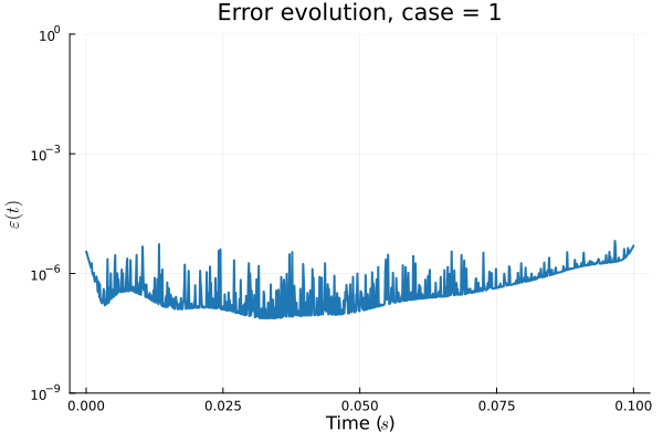
1D Advection: New Architecture
Training error
Evolution error
1D KS: New Architecture
Training error
Evolution error

Updates 04/04/24
Nonlinear Manifold Reduced Order Modeling with Neural Fields
Existing methods
- PCA based methods don't work well for transport problems
- Autoencoder based methods have large training/evaluation cost
- Implicit Neural Representations (INRs) suffer from non-smooth interpolations, and either learn dynamics from data, or use inaccurate spatial derivatives
New Contributions
- Solve the problem with non-smooth interpolation with INRs
- A smooth interpolation preserves higher order derivatives of the target function, which we compute exactly with AD
Progress this week
- Update write up, update figures
- Made a tweak in the algorithm:
- Use nonlinear solver to get initial condition
- that gives slightly better results. Want your input on whether to include this or not.
Writing Plan
- Abstract [done]
- Introduction [done]
- motivation
- lit review
- contributions [done]
-
- Manifold learning
- problem formulation
- encoder free
- smoothing
- Latent space dynamics [done]
- Galerkin projection
- Multi-stage time-steppers
- Manifold learning
- Experiments [done]
- 1D / 2D viscous Burgers
- 1D / 2D advection
- 1D Kuramoto-Sivashinsky
- Results []
- Conclutions []
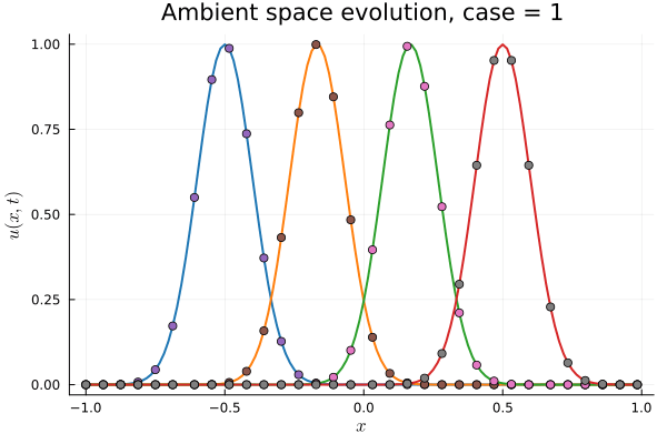
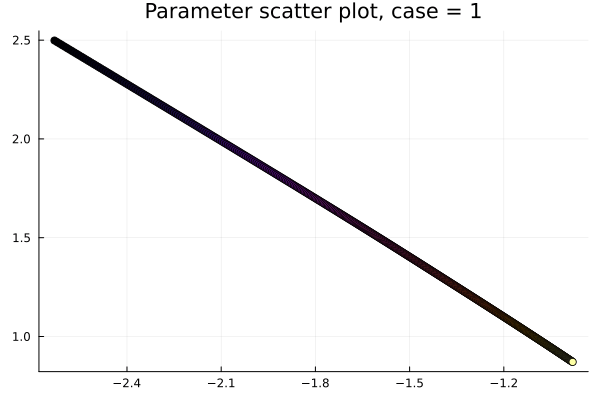
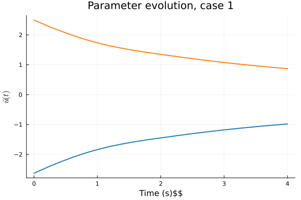
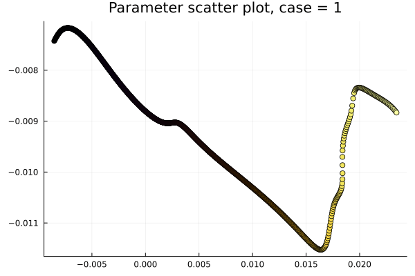
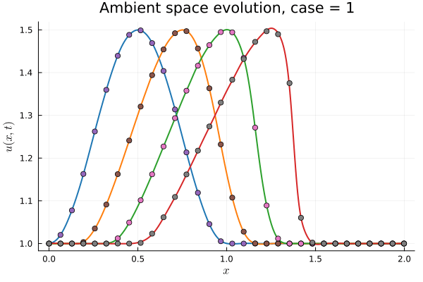
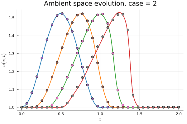
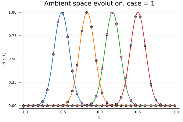
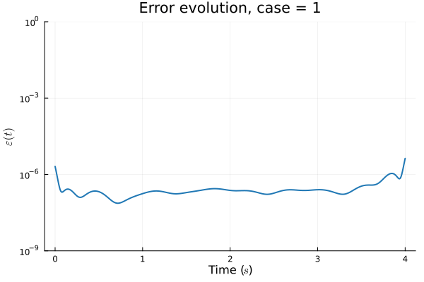
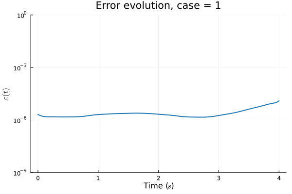
Advection 1D
Old
New
Advection 2D
Old
New
Burgers 1D
Old
New
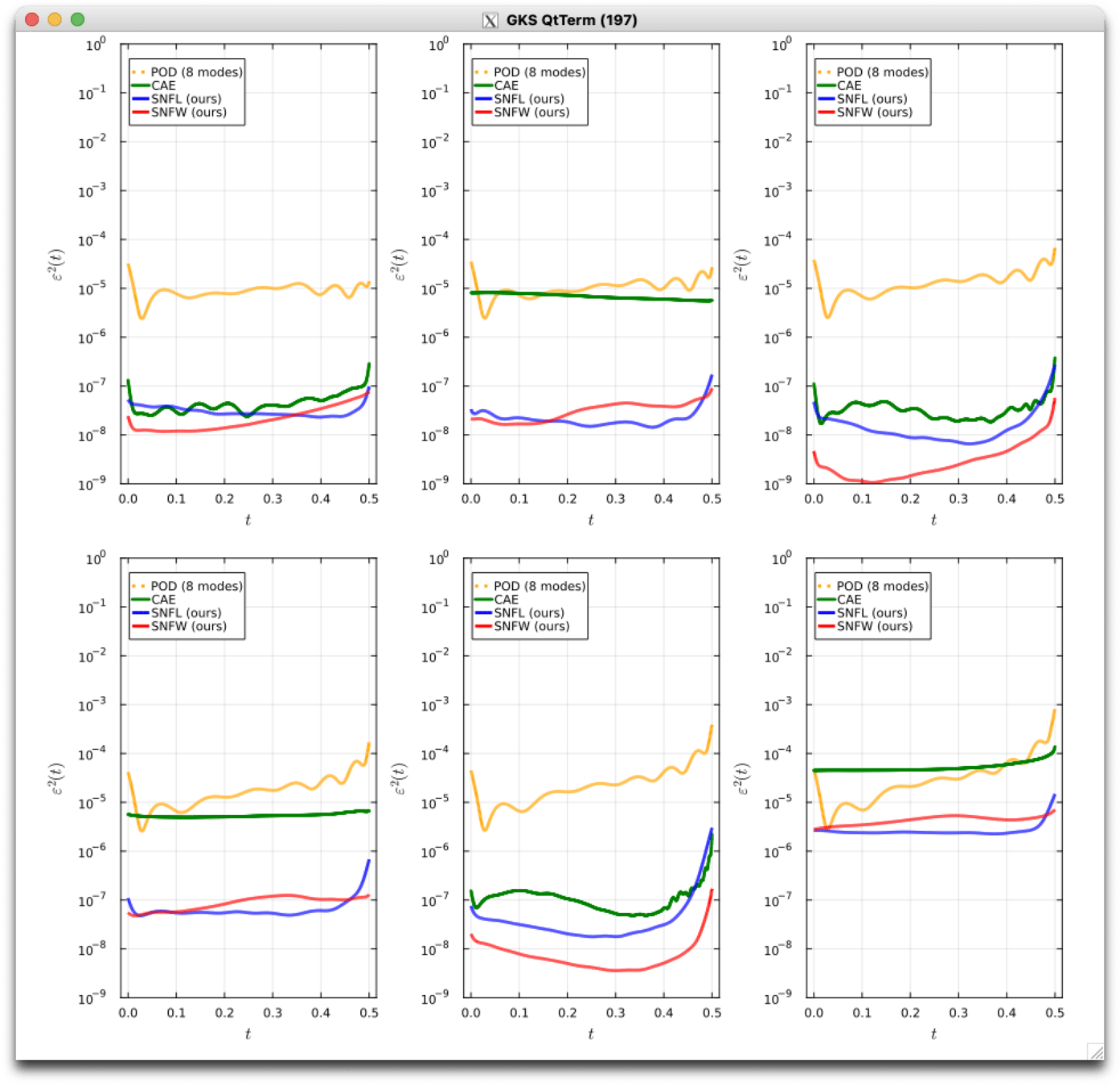
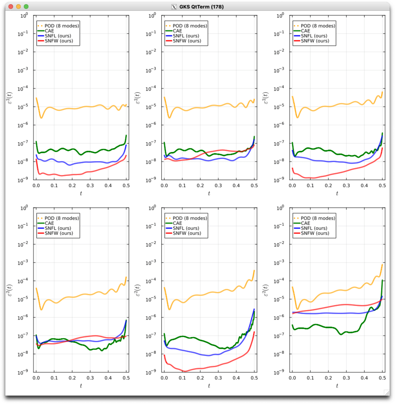
Burgers 2D
Old
New


KS 1D
Old
New