advisor_meetings

Advisor Meeting

MAR 23, 2023

Vedant Puri

https://github.com/vpuri3

Mechanical Engineering, Carnegie Mellon University

Advisors: Prof. Burak Kara, Prof. Jessica Zhang

Agenda

Motivation
- Closing the design-analysis loop
- Solve PDEs in complex geometries
Project Ideas
- ML Accelerated Meshing
- Isogeometric Analysis
- PDE surrogate models
- Orthogonal Polynomials
Goal
- Software product
- Novel algorithm, implementation

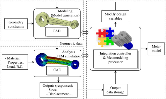
Motivation: close the loop in Computer-Aided-Engineering Cycle

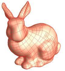
Boundary-reps

NURBS

Exact geometry

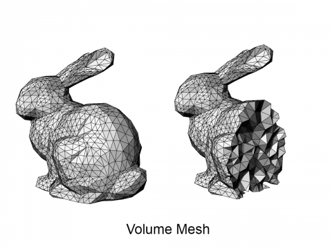
Volume mesh

Linear tets, hexes

Inexact geometry

Automated optimization loop

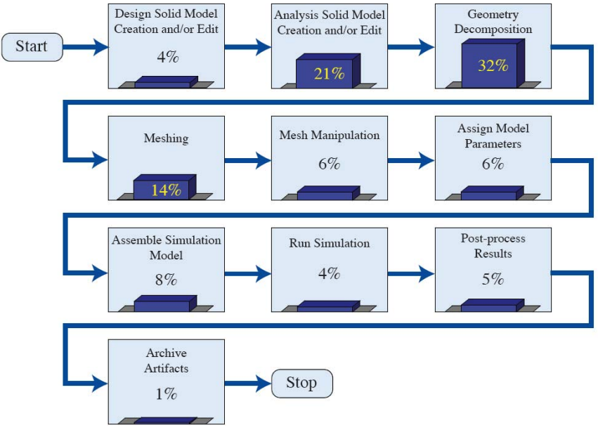
Geometry discretization is a major bottleneck

manual

error-prone

nonlinear

Mesh Iteration

Want: solve PDEs in complex geometries

Goal: Alleviate pain of translating between geometry representations

Implicit Geometry

Boundary-rep (NURBS)

Volume mesh (tets, hexes)

Computer aided design
All engineering applications

Numerical PDEs
Graphics
Visualization

Additive manufacturing
Level set methods
Easy to implement
Low storage

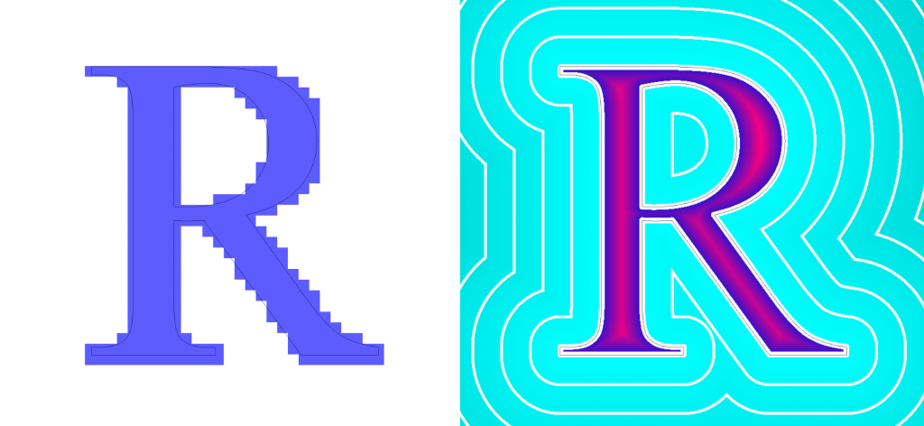
Q. What representation do neural networks like?

Topic - machine learning accelerated meshing

DistMesh (Persson, 2004)

Implicit Geometry

Volume Mesh

\Sigma_i F_i = 0\\

F = \begin{cases} k(\ell - \ell_0) & \ell < \ell_0\\ 0 & \ell \geq \ell_0\\ \end{cases}

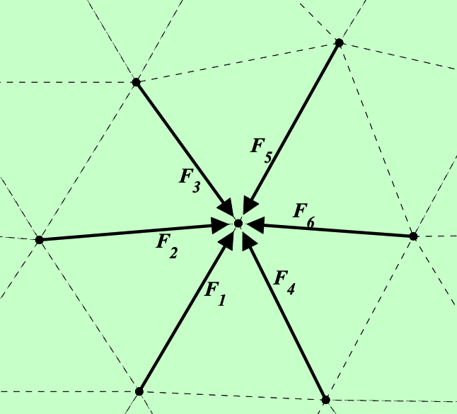
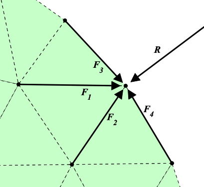
Method

Solve force balance at grid points
Update node locations
Project outside nodes back to boundary
Repeat 1-3 till equilibrium is reached

Equivalent to a Laplacian smoothing of point distribution

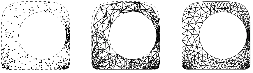
Topic - machine learning accelerated meshing

# Update mesh with gradient descent

sdf = load_geom()
x, y = generate_rand_pts(sdf)

Nepochs = 100
learning_rate = 0.01

function loss(mesh)
  # enter heuristics here
  return loss_val
end

for i = 1:Nepochs
  mesh = triangulate(x, y)
  resi = loss(mesh)

  resi < tol && break
  
  dx, dy = gradient(resi)

  x = x + dx * learning_rate
  y = y + dy * learning_rate
  
  x, y = project_boundary_nodes(x, y, sdf)
end

Update node locations with gradient descent

Heuristics:

(PDEs) Eigenvalues of \(\Delta\), residual of \(\Delta u = 1\)
Point density near boundary
Element aspect ratio, mesh grading
Matching boundary curvature

Implicit Geometry

Volume Mesh

Topic - machine learning based PDE surrogates

Motivation

We care about the physics of the problem, not the solution value at every grid point
A global PDE solve seems unnecessary for simulating physics

Goal

Use neural networks to "learn" physics
Develop architectures that respect the properties of the system. Eg.
1. convolutions respect locality
2. transformers are self-learning (attention)
Use differentiable programming to tackle nested high dimensional problems in computational workflows

Orthogonal Functions	Deep Neural Networks

Aside - ML beats the Curse of Dimensionality-ish

f = \tilde{f} + \mathcal{O}(h)

\tilde{f}(x) = \Sigma_{i=1}^N f_i \phi_i(x)

\tilde{f}(x) = Z_L \circ (\dotsc (\sigma Z_0(x)))

\( N \) parameters, \(M\) points

\( h \sim N^{-c/d} \)

\( h \sim 1 / N \) (for 2-layer networks)

\( N \) points

\( \dfrac{d}{dx} \tilde{f}\sim \mathcal{O}(N^2) \) (exact)

\( \dfrac{d}{dx} \tilde{f} \sim \mathcal{O}(N) \) (exact, AD)

\( \int_\Omega \tilde{f} dx \sim \mathcal{O}(N) \) (quadrature, exact)

(Weinan, 2020)

\( \int_\Omega \tilde{f} dx \sim \mathcal{O}(M) \) (Monte-Carlo, approx)

Aside - our goal is to add ML to the simulation pipeline

Mesh

\(A\underline{u} = M\underline{f} \)

Domain

Governing Equation

Boundary Constraint

\( NN_\theta \)

Discretization

\( \dfrac{d}{dt} \underline{u} = f(\underline{u}) \)

Solving

Discrete Problems

\(u(\underline{x},t) \)

\(u(\underline{x}) \)

Solution

Loss

Backpropogation

Data

\( NN_\theta \)

Linear Solver

Time-Stepper

Need high-level, fast, AD-compatible software ecosystem!

Aside - We are building an differentiable PDEs ecosystem

Strategy: Build out a unified PDEs ecosystem for Julia SciML!

Abstractions

Composable

AD support

Fast solvers

DL ecosystem

Large (NNs + solvers)

Multiple discretizations

Wants

Fast adjoints

Method

Interoperability

Optimized methods

High performance

High level

Unified PDEs interface

Wrap SOTA solvers

ML based discrs

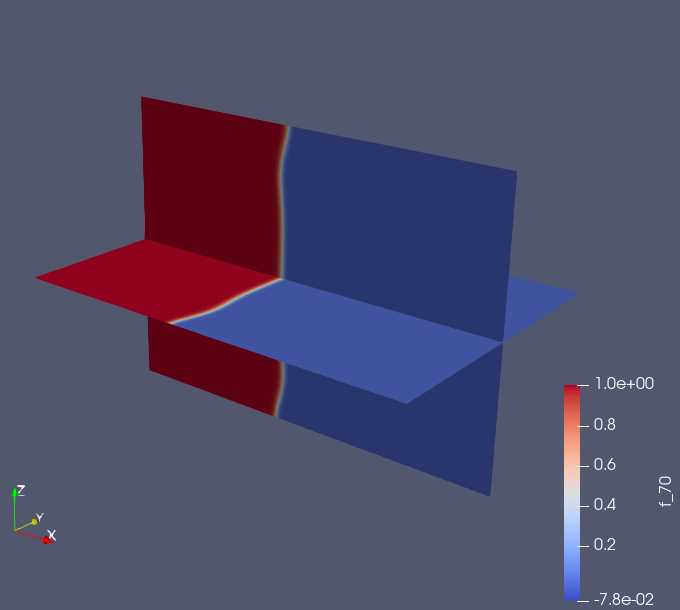
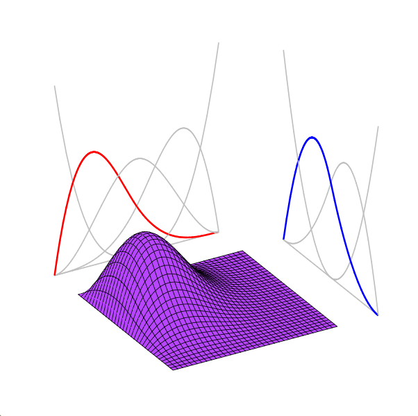
PDE Surrogates - Learning the closure to Burgers turbulence

\partial_t u + u \partial_x u = \nu \partial_x ^2 u, x\in\mathbb{R}

\partial_t \bar{u} + \bar{u} \partial_x \bar{u} = \nu \partial_x ^2 \bar{u} - \frac{1}{2}\overline{u'^2}

u = \bar{u} + u'

,\,\nu = 0.01

Closure Model

Deterministic

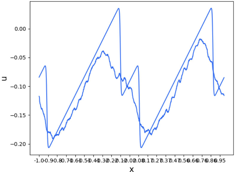
Shocks

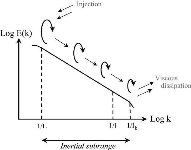
Energy Cascade

\eta := \text{NN}_\theta(u)

Eddy Viscosity Model

Vanilla Neural Network

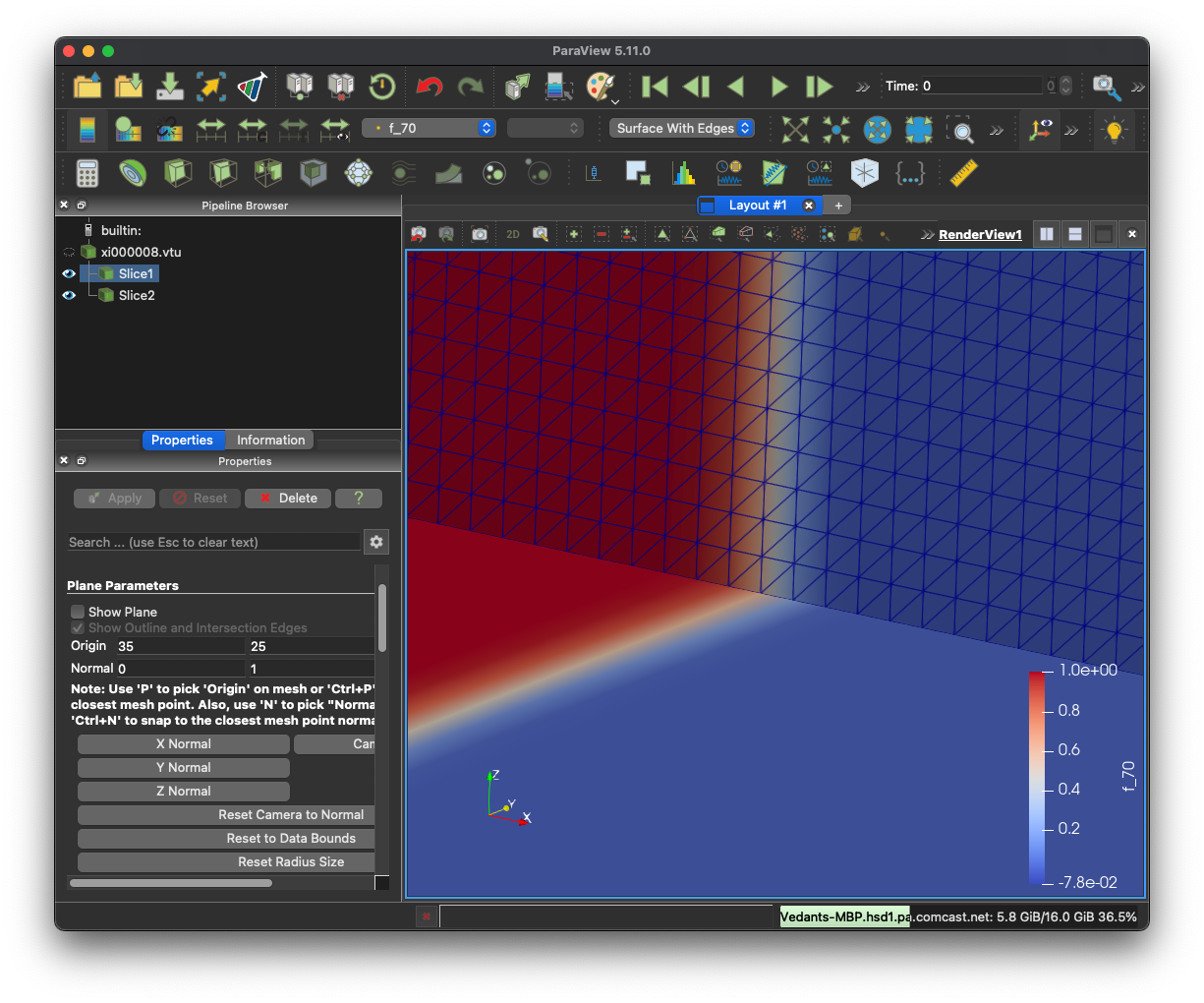
\partial_t\nu_T + \alpha_\theta(\bar{u}\partial_x \nu_T) = \beta_(\theta\nu\partial_{xx}\nu_T)

\eta := \partial_x(\nu_T\partial_x\bar{u})

PDE Surrogates - machine learning has an I/O problem

Problem: DNNs produce noisy output.

Solution: SOTA architectures use geometry respecting convolutions

Graph NN

Convolution NN

Convolution autoencoder

\begin{bmatrix} \vec{x} \\ \cdot \\ \cdot \end{bmatrix}

Latent space embedding

Convolution decoder

\begin{bmatrix} \vec{u} \end{bmatrix}

Field output

Fourier Neural Operators

u(x) = \text{NN}(x)

PDE Surrogates - convolutions

For PDEs on meshes,

What geometry representation to use?
What is the relevant convolution?
How to translate between meshes?
How to impose boundary conditions?

(If you know the convolution, the output is guaranteed to be smooth)

PDE Surrogates - we take inspiration from finite-element method

u(x) = \Sigma_{e=1}^E\Sigma_{i=1}^n u_{ie} \psi_{ie}(x)\phi_e(x)

Partition of unity

Smooth basis

Convolution

\begin{bmatrix} \vec{x} \\ d \\ \cdot \end{bmatrix}

Latent space embedding

DNN

\{\phi_e\}_{e}

DNN

\begin{bmatrix} \psi_{ie} \end{bmatrix}_{i,e}

DNN

\begin{bmatrix} u_{ie} \end{bmatrix}_{i,e}

.* d

Softmax

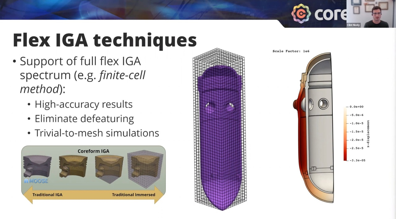
Topic - isogeometric analysis

Advisor Meeting

MAY 10, 2023

Vedant Puri

https://github.com/vpuri3

Mechanical Engineering, Carnegie Mellon University

Advisors: Prof. Burak Kara, Prof. Jessica Zhang

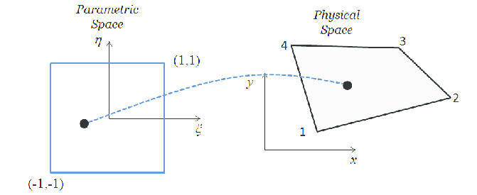
Geometry Operator Learning

Want to solve PDEs in complex geometries
Use an isoparametric mapping to parameterize geometry
Form linear system (Galerkin projection, collocation method)
Solve linear system where dependence on \(\underline{x}\) may be nonlinear
We are very good at applying \(A, M\) (matrix-free). Major cost in inverting
Problem: cannot reuse information from solve process for different \(\underline{x}\)

u(r, s) = \sum_{i=1}^N u_i \phi_i(r, s)\\ x(r, s) = \sum_{i=1}^N x_i \phi_i(r, s)

A(\underline{x}) \cdot \underline{u} = M(\underline{x}) \cdot \underline{f}

Geometry Operator Learning

Existing work on NN + geometry for PDE solving
- Train on fixed discretization, BC
- Accepts/predicts coefficients to smooth basis
- DNN \(\implies\) can only vary few parameters
Geometry operator learning:
- Want to solve \( A(\underline{x})\cdot\underline{u}=M(\underline{x})\underline{f}\) for varying \(\underline{x}\)
- Learn the discretized inverse operator and apply it to \(\underline{f}\)
- (LATER) Apply boundary condition using restriction/extension operator

(Deep) Neural Network

\underline{x}

\underline{f}

\underline{u}

\left( A^{-1}M \right)(\underline{x}) \cdot \underline{f}

(Deep) Neural Network

\underline{x}

\underline{u}

Discussion

Advantages
- Maintains linear structure of the problem
- Can save the geometry encoding offline
Problems
- Operator learning requires a lot of data
- Hard: Want to learn \( N\times N\) matrix from \(N\times 1\) vector
- How to store/apply? Need a compressed form of the matrix
How does it function operationally?
- Predict the first K singular vectors of \( A^{-1}M \)?
- Predict a sequence of convolutions?

Sandbox: start with 1D Fourier method

Keep problem size small for fast iterations
No need to worry about boundary condition
Differentiation is a diagonal operation
Discretization scheme
- Collocation
- Galerkin Projection

u(r) = \sum_{i=1}^N \hat{u}_i \exp{ikr}\\ x(r) = \sum_{i=1}^N \hat{x}_i \exp{ikr}

-\Delta u = f \implies \Sigma_{i, j}\int_{\hat{\Omega}} \nabla\phi_i\cdot \nabla \phi_j |J| dr = \Sigma_{i, j}\int_{\hat{\Omega}} \phi_i\phi_j |J| dr

\iff \left(\mathbf{J}^{-1}\mathbf{D_r}\underline{v}\right)^T |\mathbf{J}| M \left(\mathbf{J}^{-1}\mathbf{D_r}\underline{u}\right) = \underline{v}^T |\mathbf{J}| M \underline{u}

-\Delta u = f \implies -\Sigma_i \Delta u_i\phi_i = \Sigma_{i} f_i \phi_i \implies -(J^{-1}D_r)^2\underline{u} = \underline{f}

In 2D

Text

-\Delta u = f \implies \Sigma_{i, j}\int_{\hat{\Omega}} \nabla\phi_i\cdot \nabla \phi_j |J| dr = \Sigma_{i, j}\int_{\hat{\Omega}} \phi_i\phi_j |J| dr

\iff \left(\mathbf{J}^{-1}\mathbf{D_r}\underline{v}\right)^T |\mathbf{J}| B \left(\mathbf{J}^{-1}\mathbf{D_r}\underline{u}\right) = \underline{v}^T |\mathbf{J}| M \underline{u}

\mathbf{J} = \begin{bmatrix} X_r & Y_r\\ X_s & Y_s \end{bmatrix}, \mathbf{D_r} = \begin{bmatrix} D_r\\ D_s \end{bmatrix}

Advisor Meeting

MAY 24, 2023

Vedant Puri

https://github.com/vpuri3

Mechanical Engineering, Carnegie Mellon University

Advisors: Prof. Burak Kara, Prof. Jessica Zhang

Geometry Operator Learning

Want to solve \( A(\underline{x})\cdot\underline{u}=M(\underline{x})\underline{f}\) for varying \(\underline{x}\)
Learn the mapping \(\underline{x} \to (A^{-1}M(\underline{x})) \)
Apply the inverse operator to \(\underline{f}\)

\left( A^{-1}M \right)(\underline{x}) \cdot \underline{f}

Neural Network

\underline{x}

\underline{u}

NN = Chain(
    Dense(N, N, tanh),
    Dense(N, N, tanh),
    Dense(N, N, tanh),
    Dense(N, N),
)

function fwd_pass(params, x, f)
	AinvM = NN(params)(x)
	upred = AnvM * f
    return upred
end

Details

Data: triplets \((\underline{x}, \underline{f}, \underline{u})\)
Model: use vanilla DNN to predict matrix
Represent \(A^{-1}M\) as full matrix

Experiment 1 - diagonal system

Predict only the diagonal elements
True mapping: \( \texttt{x} \to \texttt{1 ./ (x .* x .* d}) \)
Data: 100 unique \(\underline{x}, \underline{u}\), i.e. 10,000 pairs for train/test sets
10k epochs with Adam optimizer

(\texttt{diag(x .* x .* d)} \cdot u = I \cdot f

N = 16

NN = Chain(
    Dense(N, N, tanh),
    Dense(N, N, tanh),
    Dense(N, N, tanh),
    Dense(N, N),
)

function loss(params, x, f, utrue)
	upred = fwd_pass(params, x, f)
    
    norm(upred - utrue, 2)
end

function fwd_pass(params, x, f)
	d = NN(params)(x)
    D = Diagonal(d)
	upred = D * f
    return upred
end

Experiment 1 - diagonal system

(\texttt{diag(x .* x .* d)} \cdot u = I \cdot f

@time p = train(_loss, p; opt = Adam(1f-2), E = 500)
@time p = train(_loss, p; opt = Adam(1f-3), E = 7500)
@time p = train(_loss, p; opt = Adam(1f-4), E = 2000)

TEST: LOSS: 258.62992872, meanAE: 0.53594627, maxAE: 1.93666885 

### TRAIN LOOP 1 ###
Iter 500: LOSS: 1.26371044, meanAE: 0.00199481, maxAE: 0.01653739
 10.948193 seconds (23.98 M allocations: 16.016 GiB, 5.34% gc time, 60.50% compilation time)

### TRAIN LOOP 2 ###
Iter 7000: LOSS: 0.10834251, meanAE: 0.00021605, maxAE: 0.000802
 62.686785 seconds (3.72 M allocations: 203.839 GiB, 8.89% gc time)

### TRAIN LOOP 3 ###
Iter 2500: LOSS: 0.01370436, meanAE: 2.405e-5, maxAE: 0.00021251
 21.679660 seconds (1.33 M allocations: 72.838 GiB, 8.30% gc time)

### TEST STATS ###
TEST: LOSS: 0.02013022, meanAE: 3.059e-5, maxAE: 0.00086486

Experiment 2 - 1D Fourier Collocation

Predict full matrix
Data: 100 unique \(\underline{x}, \underline{u}\), i.e. 10,000 pairs for train/test sets. Generate data by truncating high freq component of randomly generated vectors
10k epochs with Adam optimizer

(J^{-1} (F^{-1}\hat{D} F) \cdot J^{-1} (F^{-1}\hat{D} F)) \cdot u = M \cdot f

N = 8
N2 = N * N
NN = Chain( # predict full matrix
    Dense(N, N2, tanh),
    Dense(N2, N2, tanh),
    Dense(N2, N2, tanh),
    Dense(N2, N2),
)

function loss(params, x, f, utrue)
	upred = fwd_pass(params, x, f)
    
    norm(upred - utrue, 2)
end

function fwd_pass(params, x, f)
    m = NN(x, p, st)[1]
    M = reshape(m, (N, N, K))

    @tensorprod u[i, k] := M[i, j, k] * f[j, k]
end

Experiment 2 - 1D Fourier

@time p = train(_loss, p; opt = Adam(1f-2), E = 500)
@time p = train(_loss, p; opt = Adam(1f-3), E = 7000)
@time p = train(_loss, p; opt = Adam(1f-4), E = 2500)

TEST: LOSS: 298.75399229, meanAE: 0.83071813, maxAE: 5.42661399 

### TRAIN LOOP 1 ###
Iter 500: LOSS: 33.31564424, meanAE: 0.0878617, maxAE: 0.68316
 17.532605 seconds (3.07 M allocations: 56.414 GiB, 1.97% gc time, 3.49% compilation time)

### TRAIN LOOP 2 ###
Iter 7000: LOSS: 1.41257299, meanAE: 0.0039907, maxAE: 0.02882316
194.406308 seconds (4.33 M allocations: 645.357 GiB, 2.68% gc time)

### TRAIN LOOP 3 ###
Iter 2500: LOSS: 0.31676085, meanAE: 0.00084305, maxAE: 0.00857081
 71.722907 seconds (1.56 M allocations: 237.522 GiB, 2.44% gc time)

### TEST STATS ###
TEST: LOSS: 3.96048961, meanAE: 0.00304775, maxAE: 0.26578036

(J^{-1} (F^{-1}\hat{D} F) \cdot J^{-1} (F^{-1}\hat{D} F)) \cdot u = M \cdot f

Weekly Meeting

MAY 26, 2023

Vedant Puri

https://github.com/vpuri3

Mechanical Engineering, Carnegie Mellon University

Advisors: Prof. Burak Kara, Prof. Jessica Zhang

Updates - Geometry Operator Lerning

Problem - solve Poisson eqn over a parameterized geometry
Method - predict the inverse stiffness matrix as a function of geometry
Advantage - don't need to invert stiffness matrix for every x
Result - Predicted A^-1 as a full matrix for 1D Fourier discretization using a vanilla network
We decided to take a deep dive into machine learning before progressing further

\left( A^{-1}M \right)(\underline{x}) \cdot \underline{f}

Neural Network

\underline{x}

\underline{u}

A(\underline{x}) \cdot \underline{u} = M(\underline{x}) \cdot \underline{f}

\Delta u = f, x\in\Omega,\, u|_{\partial\Omega} = g

u(r, s) = \sum_{i=1}^N u_i \phi_i(r, s)\\ x(r, s) = \sum_{i=1}^N x_i \phi_i(r, s)

(A^{-1} M)(\underline{x}) = \texttt{NN}(x)

Updates

ML - Watching lectures from CMU DL course. Labs not available, so will do FSDL Pytorch labs
Literature review - unsure where this work belongs among established lines of research (transfer learning, operator learning). Hold off on literature review till next week when I get a better grasp on ML model space.Software implementation
Software
- Experiment code
- WIP - Write stiffness matrix over deformed geometry in 2D
- TODO next week - set up the same experiment with Dirichlet/Neumann BCs for other discretizations (Gauss-Legendre, Chebyshev)
Running bigger jobs - may i have access to a cluster?
Get access to 3420 WEH

Weekly Meeting

JUN 2, 2023

Vedant Puri

https://github.com/vpuri3

Mechanical Engineering, Carnegie Mellon University

Advisors: Prof. Burak Kara, Prof. Jessica Zhang

From last week (5/26/23)

Geometry Operator Learning - presented initial implementation on Wednesday (5/26).
- Target problem - solve lapl(u) = f over a geometry parameterized by x by predicting the inverse discretized Laplace operator u = A(x)^{-1} f on the deformed geometry: A^-1 = NN(x) .
- Results - Predicted A^-1 as a full matrix for 1D Fourier discretization using a vanilla network.
- We decided to take a deep dive into machine learning before progressing further.
- Code - Private Github repo. can give you access if you can share your GH handle.
ML - Watching lectures from CMU DL course. Their labs aren’t available to me, so I’ll do the Pytorch labs from FSDL course

From last week (5/26/23)

Software implementation
- WIP - Laplace operator on a deformed space is easy in 1D (J \ Dr * J \ Dr). Code for n-dimensions is here. I am cleaning this code, and the domain deformation interface in this PR.
- TODO next week - set up the same experiment with Dirichlet/Neumann BCs for other discretizations (Gauss-Legendre, Chebyshev).
Literature Review
- We are unsure where this work belongs among established lines of research (transfer learning, operator learning).
- Right now, I don’t understand papers involving newer ML architectures (transformers, generative models). So I’ll hold off on literature review till next week when I get a better grasp on ML model space.

Updates

ML - Watched DL lectures. up till transformers. Next: generative models, autoencoders
- Follow up with implementation: self attention for heat equation. Do we get diagonal matrix?
Software/ Implementation
- Experiment code
- PRs for gradient propagation through matrix-free operators: this, this
- PR to support fast matrix-free operators in ODE solvers
- WIP: write stiffness matrix over deformed geometry in 2D
- WIP: set up the same experiment with Dirichlet/Neumann BCs + Legendre/ Chebyshev discr

Geometry Operator Learning - Lit Review

GEOMETRY POV - aim: solve a PDE over many geometries
- Operator learning: learn the inverse Laplace operator as a function of geometry
  - Similar examples:
- Standard: learn PDE solution given as a function of geometry
  - Examples: Domain decomposition, direct approximation via PINNs
MATH POV
- Find the inverse of a parametric matrix as a function of parameters
- Example: ML --> eigenvecs, ml --> matrix factorization

Updates

Running bigger jobs - may i have access to a linux machine/ cluster?
Get access to 3414 WEH

Weekly Meeting

Literature Review on Neural Operators

JUN 7, 2023

Vedant Puri

https://github.com/vpuri3

Mechanical Engineering, Carnegie Mellon University

Advisors: Prof. Burak Kara, Prof. Jessica Zhang

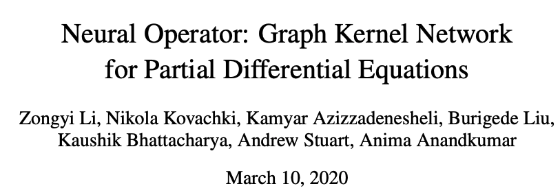
References

Li et al., Neural Operator: Graph Kernel Network for Partial Differential Equations, arXiv:2003.03485 [cs.LG]
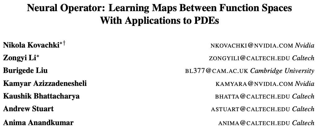
Kovachki et al., Neural Operator: Learning Maps Between Function Spaces, arXiv:2108.08481 [cs.LG]
YouTube video: Andrew Stuart - Supervised Learning for Operators

Problem Setting

(Surrogate modeling) find parameters \( \rightarrow \) solution map from given samples

Given parametric PDE,

\begin{cases} L_a(u) = -\nabla\cdot(a\nabla u) = f, & x\in\Omega\\ u|_{\partial\Omega} = 0 \end{cases}

(Training) for family of parameterized functions, \(\Psi_\theta: \mathcal{A} \times \Theta \rightarrow \mathcal{U} \), find

\text{Find } \tilde{\mathcal{\Psi}}: \mathcal{A} \rightarrow \mathcal{U} \text{ s.t. } {L}_a(\tilde{\Psi}(a)) = f,\\ \text{given } \{ a_k, \tilde{\mathcal{\Psi}}(a_k) \}_{k = 1}^K,\, a_k \sim \mu

\theta^* = \argmin_\theta \mathbb{E}^{a \sim \mu} ||\tilde{\Psi}(a) - \Psi(a; \theta)||_\mathcal{U}

= \argmin_\theta \sum_{s=1}^S ||\tilde{\Psi}(a_s) - \Psi(a_s; \theta)||_\mathcal{U}

Conventional approach: discretize then learn

Fix a grid

\mathcal{A}^h \subset \mathcal{A}, \, \mathcal{U}^h \subset \mathcal{U}

G^h = \{x_i \}_{i=1}^{N}

Learn finite neural network model \(\mathbb{R}^{N'} \rightarrow \mathbb{R}^N \)

\begin{bmatrix} a \\ \cdot \end{bmatrix}

\begin{bmatrix} \vec{u} \end{bmatrix}

\mathcal{A}^h, \mathcal{U}^h \cong \mathbb{R}^N

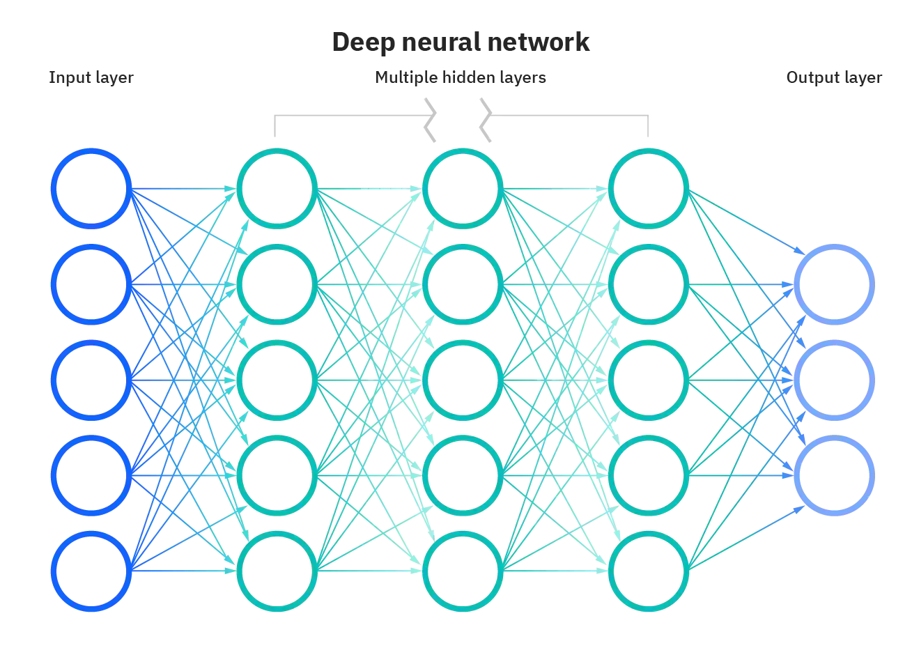
Deep Neural Network

Disadvantages:

Model implicitly learns grid dependence
Lack of generalizability/ transferability

PINNs, on the other hand, do not depend on training meshes.

But they represent the solution, \(\tilde{\Psi}(a)\) only for one instance of \(a\)

Neural operators map between Banach spaces

Map between (approximations of) Banach spaces

\Psi: \mathcal{A} \rightarrow \mathcal{U}

\mathcal{A}^{h_1}\\ \vdots\\ \mathcal{A}^{h_k}\\

\mathcal{U}^{h_1}\\ \vdots\\ \mathcal{U}^{h_k}\\

G^{h_1}

G^{h_k}

A single set of network parameters describe any \( \mathcal{A}^{h_k} \rightarrow \mathcal{U}^{h_l}\) mapping

Neural operator models

Fix \(K\) basis functions in \(\mathcal{A},\, \mathcal{U}\) space using PCA from \(\mu\)
Interpolate basis to \( \mathcal{A}^{h_a}, \mathcal{U}^{h_u}\), and put them in matrices
Train neural network to map between basis coefficients

A = \begin{bmatrix} \vdots & \vdots & \vdots \end{bmatrix}_{N_a\times K}

\Psi_\text{PCA}(a;\theta) = U \cdot \alpha(A^T \cdot a;\theta)

U = \begin{bmatrix} \vdots & \vdots & \vdots \end{bmatrix}_{N_u\times K}

DEEPONET

The basis in \( \mathcal{U}\), is learnable: \( U = U(\theta)\)
\( L(a)\) can be vector of PCA coefficients, \( A^T\cdot a\), or pointwise observations, \( \{ a(x_l)\}\)

\Psi_\text{DEEP}(a;\theta) = U(\theta) \cdot \alpha(L(a);\theta)

Aside: Green's function and integral operators

For elliptic equation \( \mathcal{L}_a \) parameterized by \(a\),

\mathcal{L}_a(G(x, y)) = \delta_y

Then \( \mathcal{L}_a(u) = f \) is solved by

u(x) = \int_\Omega G(x, y) f(y) dy

Proof:

\mathcal{L}_a(u) = \mathcal{L}_a(\int_\Omega G(x, y)f(y)dy)

= \int_\Omega \mathcal{L}_a(G(x, y))f(y)dy)

= \int_\Omega \delta_y f(y)dy)

= f

Operator models approximate Green's function

Assume a Green's function exists for \( \mathcal{L}_a \)
Approximate with sequence of global + local operations

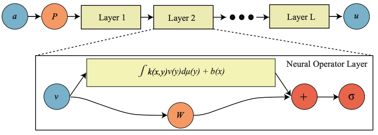
Global convolution

Pointwise transformation

Lifting operation

Graph Kernel Network

Convolution performed by graph neural network with trainable weights

v_{t+1}(x_j) = \sigma \circ \left( Wv_t(x_j) + \frac{1}{|N(x_j)|}\sum_{y\in N(x_j)}\kappa^t_\theta(x_j, y)v_t(y) \right)

\( \kappa(x, y, a(x), a(y))\)

pointwise transformation

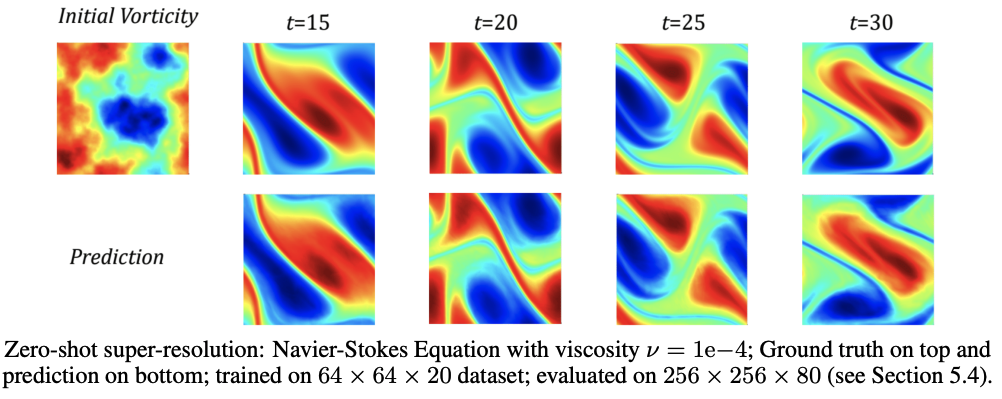
Using a spectral fourier basis has advantages

G^{6}

G^{3}

\begin{pmatrix} \widehat{u_1}^3\\ \widehat{u_2}^3\\ \widehat{u_3}^3\\ 0\\ 0\\ 0\\ \end{pmatrix} = \begin{bmatrix} 1 & 0 & 0\\ 0 & 1 & 0\\ 0 & 0 & 1\\ 0 & 0 & 0\\ 0 & 0 & 0\\ 0 & 0 & 0\\ \end{bmatrix} \begin{pmatrix} \widehat{u_1}^3\\ \widehat{u_2}^3\\ \widehat{u_3}^3\\ \end{pmatrix}

\(G^6 \leftarrow G^3 \) interpolation

\mathcal{F}(f \ast g) = \mathcal{F}^{-1}(\mathcal{F}(f)\odot\mathcal{F}(g))

Nested points in physical space
Spectral interpolation is trivial
Convolution is pointwise in spectral space
FFT makes transform \(N\log N\)

Fourier neural operator

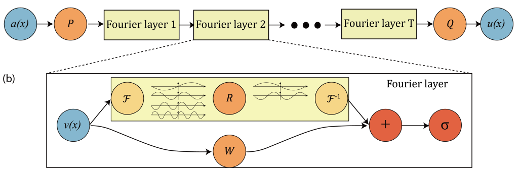
Lifting Operator

Projection Operator

Linear transform on first \(K\) Fourier modes

Local linear transform

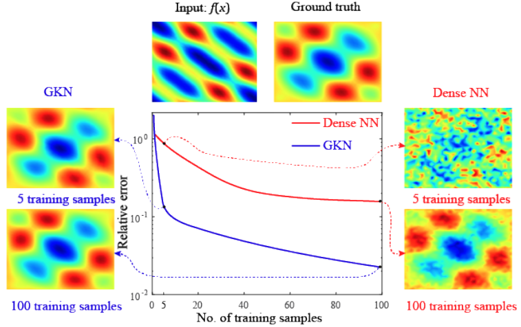
Fourier neural operator results

Advantages

Surrogate modeling/ inverse modeling - optimization requires cheap, fast solves
Closure modeling - benefits from grid independence
Speed up existing solvers with cheap initial guess/ preconditioner
- Train model on first few snapshots of a long time-integration, then use it as incomplete factorization preconditioner.

Discussion

Grid-independent approximation
Can pull many data streams, combine with experiments
Needs very few training samples

Use-Cases

Discussion

Integral operators work well for elliptical problems, but fail badly for hyperbolic problems (eg. advection equation)
Fourier not usable for practical problems

Easiest idea - replace Fourier with Chebyshev and try to involve BCs
The geometry learning problem is not truly an operator learning problem as described here. It is not grid/resolution independent

Disadvantages

Ideas - how to proceed further?

Weekly Meeting

JUN 9, 2023

Vedant Puri

https://github.com/vpuri3

Mechanical Engineering, Carnegie Mellon University

Advisors: Prof. Burak Kara, Prof. Jessica Zhang

Updates

ML crash course - done
Logistics
- Need a computer/ compute access
- Need office access (?)
Neural Operator discussion -> next

Neural Operators

Surrogate model (parameters \(\longrightarrow \) solution)

\Psi: \mathcal{A} \rightarrow \mathcal{U}

\mathcal{A}^{h_1}\\ \vdots\\ \mathcal{A}^{h_k}\\

\mathcal{U}^{h_1}\\ \vdots\\ \mathcal{U}^{h_k}\\

G^{h_1}

G^{h_k}

\begin{cases} L_a(u) = f, & x\in\Omega\\ u|_{\partial\Omega} = g \end{cases}

Unique selling point: resolution invariance

Neural Operators

Neural Operator Capabilities/ limitations

resolution invariance
fixed geometry
fixed parameter set (BC, forcing function)
Works well for elliptic equations, not so well for hyperbolic problems

Our Goals

Learn surrogate model over varying geometry
Decouple training WRT components of a PDE problem
- forcing, BC, geometry, equation parameters

Neural Operators Methodology

Approximate Green's function with NN involving only pointwise evaluations, global convolutions

\begin{cases} L_a(u) = f, & x\in\Omega\\ u|_{\partial\Omega} = 0 \end{cases}

\begin{cases} L_a(G(x, y)) = \delta(x - y), & x\in\Omega\\ u|_{\partial\Omega} = 0 \end{cases}

u(x) = \int_\Omega G(x, y) f(y) d y

As (training) discretization is refined, model approximates the continuum operator.

Fourier Neural Operator

best in class neural operator model
resolution invariance (on uniform grids)
restricted to periodic BC
not very practical (hammer searching for a nail), but very impressive results
Global convolution performed with FFT in \(\mathcal{O}(N\log N)\)

Involve BC in Neural Operators

For linear equations, eg. Poisson

\begin{cases} \Delta u = f, & x\in\Omega\\ u|_{\partial\Omega} = g \end{cases}

u(x) = \int_\Omega G(x, y) f(y) d y + \int_{\partial\Omega} \nabla \cdot G(x, y) g(y) d y

Dependence on \( f \), \( g \) is described by a linear convolution

Proposed Methodology

Utilize separate neural networks for learning BC, \(f\), and train independently
\(u_{f_0}\): Neural operator model; \(u_\text{BC}, \, u_{f-f_0} \longrightarrow\) linear convolutions

u = u_{f_0} + u_\text{BC} + u_{f-f_0}

\begin{cases} L_a(u) = f_0,\\ u|_{\partial\Omega} = 0 \end{cases}

\begin{cases} L_a(u) = 0,\\ u|_{\partial\Omega} = g \end{cases}

\begin{cases} L_a(u) = f-f_0,\\ u|_{\partial\Omega} = 0 \end{cases}

\begin{cases} L_a(u) = f, & x\in\Omega\\ u|_{\partial\Omega} = g \end{cases}

Weekly Meeting

JUN 16, 2023

Vedant Puri

https://github.com/vpuri3

Mechanical Engineering, Carnegie Mellon University

Advisors: Prof. Burak Kara, Prof. Jessica Zhang

Updates

Recap (last week):
- Neural operators literature review
  - Fourier Neural Operator best in class model
  - Combine local/global operations
  - Resolution invariant, but limited usability
- Target problem: surrogate modeling
  - Want to develop complex geometry analog
  - Separate out training for BCs, forcing
This week:
- Reread neural operator papers
- Set up first experiment to test idea

u = u_{\{a\},f_0} + u_\text{\{a\},\{g\}} + u_{\{a\},\{f\}}

\begin{cases} L_a(u) = f_0,\\ u|_{\partial\Omega} = 0 \end{cases}

\begin{cases} L_a(u) = 0,\\ u|_{\partial\Omega} = g \end{cases}

\begin{cases} L_a(u) = f-f_0,\\ u|_{\partial\Omega} = 0 \end{cases}

\begin{cases} L_a(u) = f, & x\in\Omega\\ u|_{\partial\Omega} = g \end{cases}

Nonlinear in \(a\), linear in \(g, \,f\)

Separate NNs

Experiment

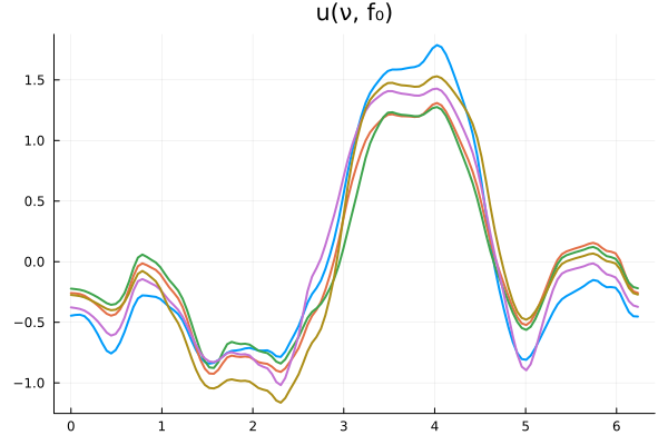
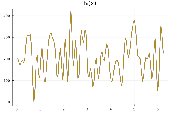
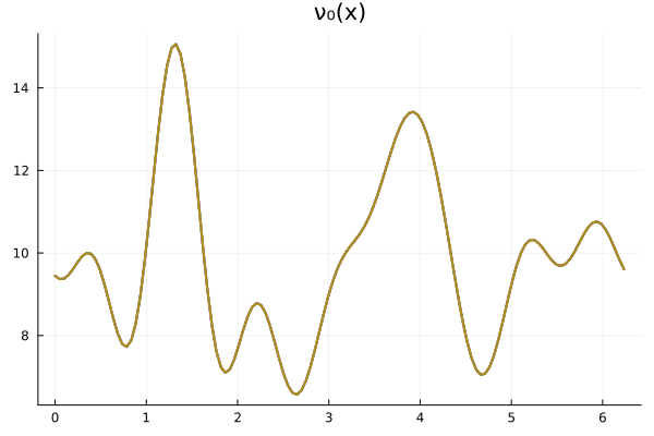
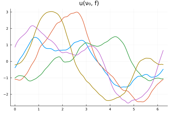
Problem: Find map \(\nu \longrightarrow u\)

\begin{cases} \nabla \cdot \nu \nabla u = f\\ u(0) = u(2\pi) \end{cases}

Superimpose distinct neural networks

u = u_{\{\nu\},f_0} + u_{\{\nu\},\{f\}}

L_\nu(u) = f_0

L_\nu(u) = f-f_0

\(N_\nu = 100, \, N_f = 100\) unique fields \( \implies 10k\) unique trajectories
\( N = 128 \) point Fourier discretization \( \implies 1.2\,\text{m}\) datapoints

Experiment Part I

Trained \(u_{\{\nu\},f_0}\) dense neural network (20k epochs, 60k params)

meanRE: 0.00029135, maxRE: 0.00173817

Solution much more dependent on \(f\) than on \(\nu\)

u = u_{\{\nu\},f_0}

L_\nu(u) = f_0

meanRE: 0.00348382, maxRE: 0.0233049

Experiment Part II (WIP)

Trained \(u_{\{a\},f_0}\) dense neural network (20k epochs, 80k params)

WIP: replace DNN with linear Fourier Neural Operator

u = u_{\nu_0,\{f\}}

L_{\nu_0}(u) = f

meanRE: 0.00500959, maxRE: 1.953022

meanRE: 1.32767527, maxRE: 1608.9298091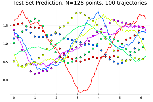

Updates

Next steps
- Implementing Fourier neural operator for Experiment 1
- Prepare for next experiment with Dirichlet BC
  - Replace Fourier discretization with Chebyshev
  - Generate data by solving boundary value problems
- Do more literature review, put it in a document
From discussion with Prof. Kara
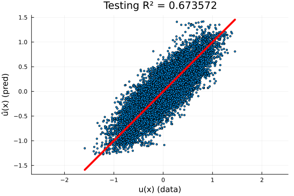
- R^2 plots
- Loss plots for train/ test sets

Proposed Methodology

u = u_{\{a\},f_0} + u_\text{\{a\},\{g\}} + u_{\{a\},\{f\}}

\begin{cases} L_a(u) = f_0,\\ u|_{\partial\Omega} = 0 \end{cases}

\begin{cases} L_a(u) = 0,\\ u|_{\partial\Omega} = g \end{cases}

\begin{cases} L_a(u) = f-f_0,\\ u|_{\partial\Omega} = 0 \end{cases}

Linera convolutions in \(g, \,f\)

Independent training

Separate NNs

\(N_a\) samples

\(N_a\cdot N_g\) samples

\(N_a\cdot N_f\) samples

Weekly Meeting

JUN 23, 2023

Vedant Puri

https://github.com/vpuri3

Mechanical Engineering, Carnegie Mellon University

Advisors: Prof. Burak Kara, Prof. Jessica Zhang

Updates

\begin{cases} L_a(u) = f, & x\in\Omega\\ u|_{\partial\Omega} = g \end{cases}

Goal

Find (surrogate) map \( a \longrightarrow u \) that is

Cheap to compute
Generalizes with little data
Not looking for very high accuracy

Updates from this week

Implement Fourier Neural Operator model, compare with other networks
Had some difficulty training, got past that.
Wrote bilinear neural operator layer

Next Steps

Construct Chebyshev Neural Operator
Next experiment: separate out training for BCs, forcing

Neural Operator Kernel

Convolution Kernel

\begin{bmatrix} x \end{bmatrix}

\( Wx\)

\(\mathcal{F}^{-1}W \widehat{x} \)

\begin{bmatrix} y \end{bmatrix}

Local Kernel

\sigma

Experiment

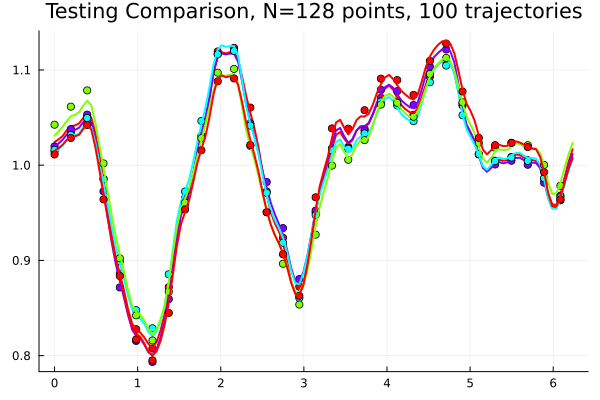
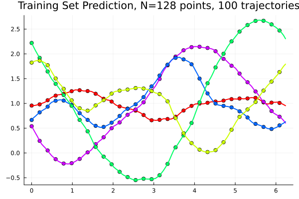
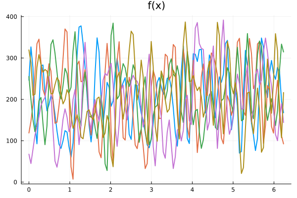
Problem: Find map \((\nu,f) \longrightarrow u\)

\begin{cases} -\nabla \cdot \nu \nabla u = f\\ u(0) = u(2\pi) \end{cases}

Generate data with \( N = 128 \) point Fourier discretization


# Trajectories	100	100	50 * 50
# Points	12,800	12,800	320,000

-\nabla \cdot \nu_0 \nabla u = f

-\nabla \cdot \nu \nabla u = f_0

-\nabla \cdot \nu \nabla u = f

ML models
- Pointwise DNN
- Sequence-to-sequence DNN
- Fourier Neural Operator

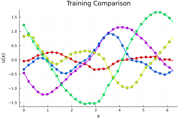
Experiment I: \(-\nabla \cdot \nu_0 \nabla u = f \)

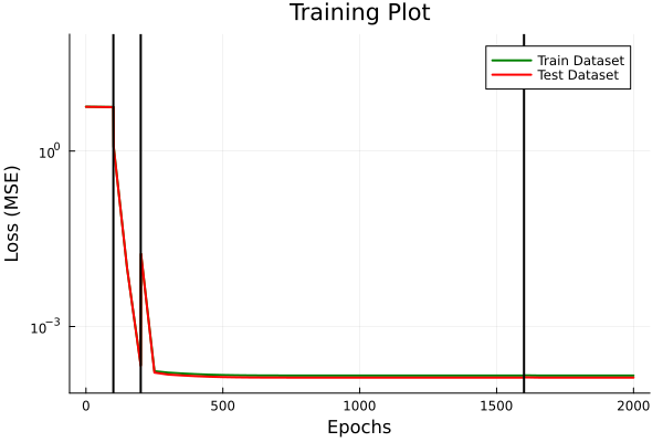
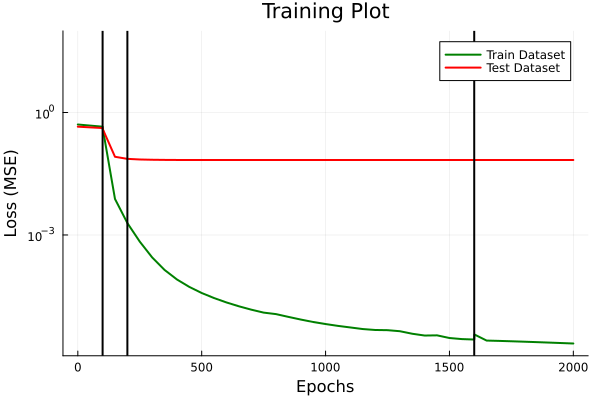
Seq-2-seq DNN

Fourier Neural Operator

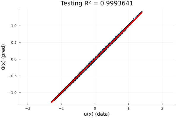
64 parameters
Single FNO spectral convolution layer
\(R^2=0.999\) on test set

82k parameters
Five \(128\times128\) hidden layers
\(R^2=0.67\) on test set

Experiment I: \(-\nabla \cdot \nu_0 \nabla u = f \)

Seq-2-seq DNN

Fourier Neural Operator

Experiment I: \(-\nabla \cdot \nu_0 \nabla u = f \)

Seq-2-seq DNN

Experiment I: \(-\nabla \cdot \nu_0 \nabla u = f \)

Fourier Neural Operator

Experiment II: \(-\nabla \cdot \nu \nabla u = f_0 \)

Seq-2-seq DNN

Fourier Neural Operator

32 parameters
Single FNO spectral convolution layer
\(R^2=0.98\) on test set

66k parameters
Three \(128\times128\) hidden layers
\(R^2=0.98\) on test set

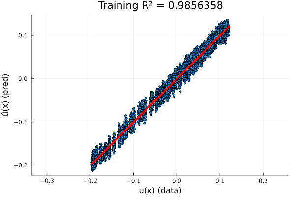
Full Experiment: \(-\nabla \cdot \nu \nabla u = f\)

Fourier Neural Operator

Pointwise DNN

48 parameters
Single FNO spectral convolution layer
\(R^2=0.987\) on test set

64k parameters
Eight \(64\times64\) hidden layers
\(R^2=0.07\) on test set

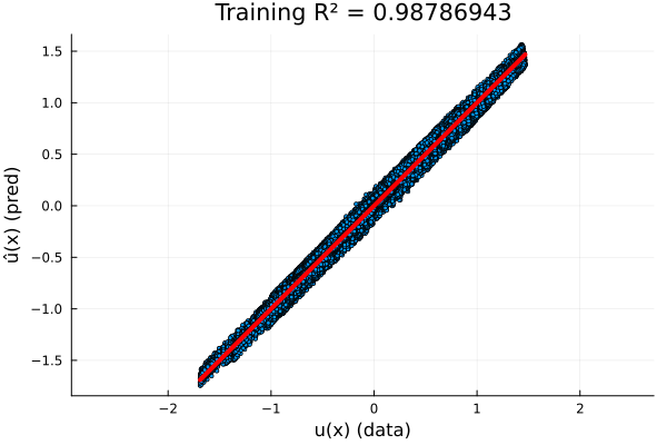
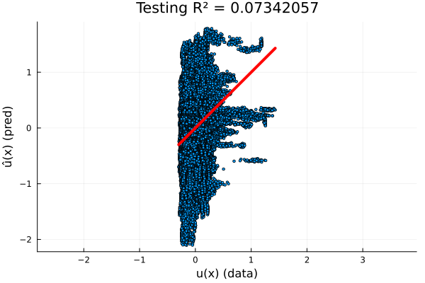
Full Experiment: \(-\nabla \cdot \nu \nabla u = f\)

Fourier Neural Operator

Pointwise DNN

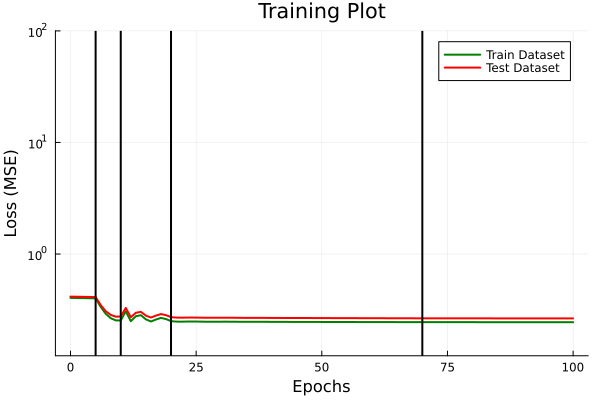
Discussion

Disucssion

Fourier Neural Operator implementation performs better than other tested models, and does so with fewer parameters.

Next Steps

Test model splitting idea
- Network \(u_{\{\nu\},f_0}\) nonlinear in \(\nu\)
- Network \(u_{\{\nu\},f}\) nonlinear in \(\nu\), linear in \(f\)
Develop bilinear neural operator layer!

\begin{cases} -\nabla \cdot \nu \nabla u = f\\ u(0) = u(2\pi) \end{cases}

u = u_{\{\nu\},f_0} + u_{\{\nu\},\{f\}}

L_\nu(u) = f_0

L_\nu(u) = f-f_0

Neural Operator

\begin{bmatrix} \nu \\ \vec{x} \end{bmatrix}

Operator Kernel

\begin{bmatrix} f \end{bmatrix}

Bilinear

Operator Kernel

\begin{bmatrix} u \end{bmatrix}

Affine

Linear

\sigma

Bilinear Operator Kernel Layer

Bilinear Convolution Kernel

\begin{bmatrix} x \end{bmatrix}

\begin{bmatrix} y \end{bmatrix}

\( x^TWy\)

\(\mathcal{F}^{-1}(\widehat{x}^T W \widehat{y}) \)

\begin{bmatrix} z \end{bmatrix}

Bilinear Local Kernel

Bilinear Operator Layer

Single DNN for linear, nonlinear branches, with bilinear convolution layer for fusing results
300 parameters (mostly in the DNNs)
\(R^2 = 0.997\) (test set)

Weekly Meeting

JUL 7, 2023

Vedant Puri

https://github.com/vpuri3

Mechanical Engineering, Carnegie Mellon University

Advisors: Prof. Burak Kara, Prof. Jessica Zhang

Updates

\begin{cases} L_a(u) = f, & x\in\Omega\\ u|_{\partial\Omega} = g \end{cases}

Target Problem

Find (surrogate) map \( a \longrightarrow u \) that is

Efficient, generalizes with sparse data

Updates

Implement Fourier Neural Operator (FNO)
Modified FNO model for linear PDEs (developed bilinear layer)
Experiments with Bilinear layer
(work in progress) experiment: parameter splitting
(work in progress) backward pass for Discrete Cosine Transform (i.e. Chebyshev transform)

Next Steps

Experiments becoming too large for my laptop - need machine with GPU
Involve boundary conditions with Chebyshev transform

Neural Operator Kernel

Convolution Kernel

\begin{bmatrix} x \end{bmatrix}

\( Wx\)

\(\mathcal{F}^{-1}W \widehat{x} \)

\begin{bmatrix} y \end{bmatrix}

Local Kernel

\sigma

Bilinear Neural Operator Layer

\begin{bmatrix} \nu \\ \vec{x} \end{bmatrix}

Operator Kernel

\begin{bmatrix} f \end{bmatrix}

Bilinear

Operator Kernel

\begin{bmatrix} u \end{bmatrix}

Affine

Linear

\sigma

\begin{cases} -\nabla \cdot \nu \nabla u = f\\ u(0) = u(2\pi) \end{cases}

\sigma

Bilinear Neural Operator Layer

\begin{bmatrix} \nu \\ \vec{x} \end{bmatrix}

Affine

\begin{cases} -\nabla \cdot \nu \nabla u = f\\ u(0) = u(2\pi) \end{cases}

Affine

Bilinear Operator Kernel

Bilinear Convolution Kernel

\begin{bmatrix} x \end{bmatrix}

\begin{bmatrix} y \end{bmatrix}

\( x^TW_\text{loc}y\)

\(\mathcal{F}^{-1}(\widehat{x}^T W_\text{conv} \widehat{y}) \)

\begin{bmatrix} z \end{bmatrix}

Bilinear Local Kernel

Bilinear Operator Layer

Single DNN for linear, nonlinear branches, with bilinear convolution layer for fusing results
300 parameters (mostly in the DNNs)
\(R^2 = 0.997\) (test set)

Experiment Setup

Problem: Find map \((\nu,f) \longrightarrow u\)

\begin{cases} -\nabla \cdot \nu \nabla u = f\\ u(0) = u(2\pi) \end{cases}

Generate data with \( N = 128 \) point Fourier discretization


# Trajectories	100	100	32 x 32
# Points	12,800	12,800	131,072

-\nabla \cdot \nu_0 \nabla u = f

-\nabla \cdot \nu \nabla u = f_0

-\nabla \cdot \nu \nabla u = f

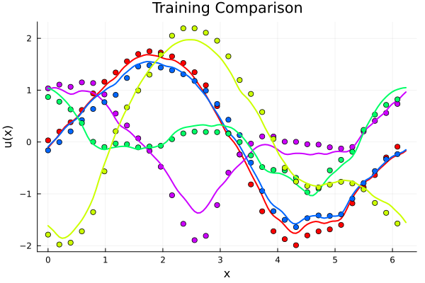
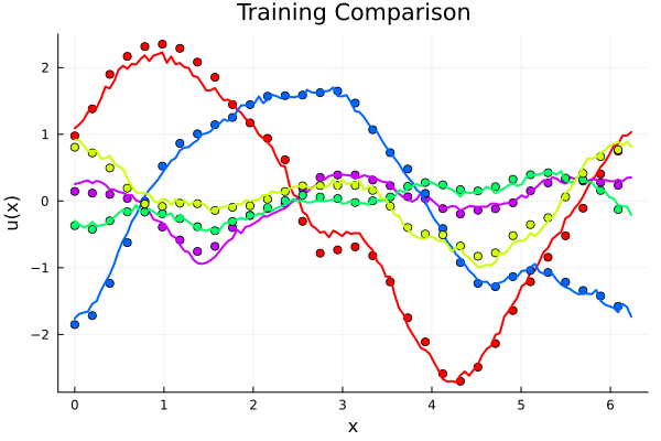
Experiment Setup: \(-\nabla \cdot \nu \nabla u = f_0\)

Experiment Setup: \(-\nabla \cdot \nu_0 \nabla u = f\)

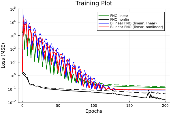
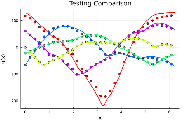
Experiment: \(-\nabla \cdot \nu \nabla u = f \)

Architecuters

Nonlinear FNO
Linear FNO
Bilinear FNO (linear / linear)
Bilinear FNO (linear / nonlinear)

[x, nu, f] -> BatchNorm() -> Dense(3 , w, tanh) -> OpKernel(w, w, m, tanh)
  	   -> OpKernel(w, w, m, tanh) -> Dense(w , 1) -> u

[x, nu, f] -> Dense(3 , w) -> OpKernel(w, w, m) -> Dense(w , 1) -> u

[x, nu] -> BatchNorm(c) -> Dense(c, w, tanh), OpKernel(w, w, m) ↘
								 OpConvBilinear(w, w, m, 1) -> u
                                             [f] -> Dense(c, w) ↗

[x, nu] -> Dense(c, w), OpKernel(w, w, m) ↘
					   OpConvBilinear(w, w, m, 1) -> u
                       [f] -> Dense(c, w) ↗

Experiment: \(-\nabla \cdot \nu \nabla u = f \)

Linear FNO
- \(R^2 = 0.91, 0.92 \) (train/ test)
Nonlinear FNO
- \(R^2 = 0.98, 0.97 \) (train/ test)
Bilinear FNO (linear / linear)
- \(R^2 = 0.94, 0.95 \) (train/ test)
Bilinear FNO (linear / nonlinear)
- \(R^2 = 0.94, 0.95 \) (train/ test)

Discusion

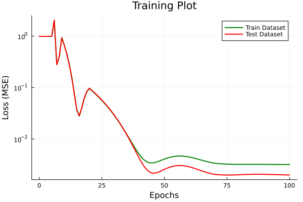
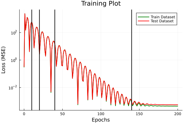
Oscillations arise in linear models only
Large gradients at training onset push parameter set far away from optimum

Next Steps

Workin on

(work in progress) experiment: parameter splitting
(work in progress) backward pass for Discrete Cosine Transform (i.e. Chebyshev transform)

Next Steps

Experiments becoming too large for my laptop - need machine with GPU
Involve boundary conditions with Chebyshev transform

TODO

Compare results with literature for 1D diffusion (PDEBench), or 2D bench + Darcy flow
Lit review on ML optimization dynamics
Implement using julia because... (justify choice of platform)
Run on PSC Bridges
What are the novel contributions? 1 page

Parameter Splitting

Network \(u_{\{\nu\},f_0}\) nonlinear in \(\nu\)
Network \(u_{\{\nu\},f}\) nonlinear in \(\nu\), linear in \(f\)

\begin{cases} -\nabla \cdot \nu \nabla u = f\\ u(0) = u(2\pi) \end{cases}

u = u_{\{\nu\},f_0} + u_{\{\nu\},\{f\}}

L_\nu(u) = f_0

L_\nu(u) = f-f_0

Train on \(N_\nu\cdot N_f\) trajectories

Train on \(N_\nu\)

trajectories

Weekly Meeting

JUL 19, 2023

Vedant Puri

https://github.com/vpuri3

Mechanical Engineering, Carnegie Mellon University

Advisors: Prof. Burak Kara, Prof. Jessica Zhang

Updates

\begin{cases} L_a(u) = f, & x\in\Omega\\ u|_{\partial\Omega} = g \end{cases}

Target Problem

Find (surrogate) map \( (x, a, f, g, \dotsc) \longrightarrow u \)

Efficient, generalizes with sparse data

So Far ( ~ 1/3 of the way there)

Experimented with Neural Operator models in 1D
Discussed parameter splitting idea for linear PDEs
Modified operator model to respect linearity (superior generalizability over some parameters)

Next Steps

Extend to 2D
Involve Boundary Conditions
Test against benchmarks

u = u_{\{a\},f_0} + u_\text{\{a\},\{g\}} + u_{\{a\},\{f\}}

\begin{cases} L_a(u) = f_0,\\ u|_{\partial\Omega} = 0 \end{cases}

\begin{cases} L_a(u) = 0,\\ u|_{\partial\Omega} = g \end{cases}

\begin{cases} L_a(u) = f-f_0,\\ u|_{\partial\Omega} = 0 \end{cases}

\(N_a\) samples

\(N_a\cdot N_g\) samples

\(N_a\cdot N_f\) samples

Neural Operator Layer

Convolution Kernel

\begin{bmatrix} x \end{bmatrix}

\( W_\text{loc}x+b\)

\(\mathcal{F}^{-1}W_\text{conv} \widehat{x} \)

\begin{bmatrix} y \end{bmatrix}

Local Kernel

\sigma

@tullio Y_conv[co, m, b] := W_conv[co, ci, m] * X[ci, m, b]

@tullio Y_loc[co, n, b] := W_conv[co, ci] * X[ci, n, b]

Bilinear Operator Layer

Bilinear Convolution Kernel

\begin{bmatrix} x \end{bmatrix}

\begin{bmatrix} y \end{bmatrix}

\( x^TW_\text{loc}y\)

\(\mathcal{F}^{-1}(\widehat{x}^T W_\text{conv} \widehat{y}) \)

\begin{bmatrix} z \end{bmatrix}

Bilinear Local Kernel

@einsum Z_conv[co, m, b] := X[c1, m, b] * W_conv[co, c1, c2, m] * Y[c2, m, b]

@einsum Z_loc[co, n, b] := X[c1, n, b] * W_loc[co, c1, c2] * Y[c2, n, b]

Modified Neural Operator Model

\begin{bmatrix} \nu \\ \vec{x} \end{bmatrix}

Operator Kernel

\begin{bmatrix} f \end{bmatrix}

Bilinear

Operator Kernel

\begin{bmatrix} u \end{bmatrix}

Affine

Linear

\sigma

\begin{cases} -\nabla \cdot \nu \nabla u = f\\ u(0) = u(2\pi) \end{cases}

\sigma

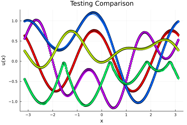
Experiment: \(-\nabla \cdot \nu \nabla u = f\)

Modified FNO

Classic FNO

16k parameters
Convolution bilinear layer
\(R^2=0.97\) on training set

25k parameters
\(R^2=0.98\) on training set

Hypothesis: Modified model should generalize better on out-of-distribution data

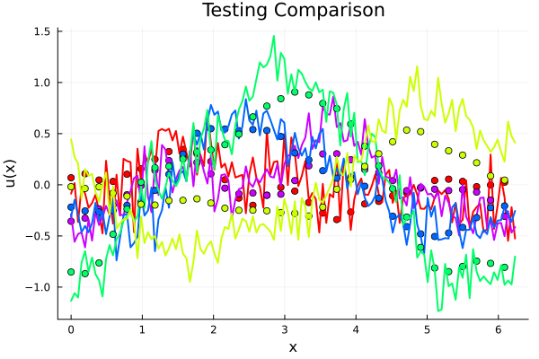
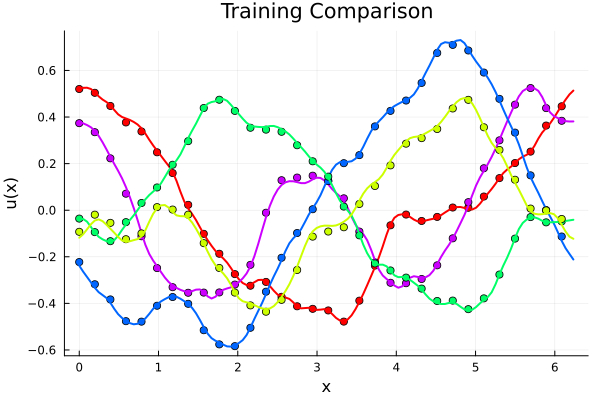
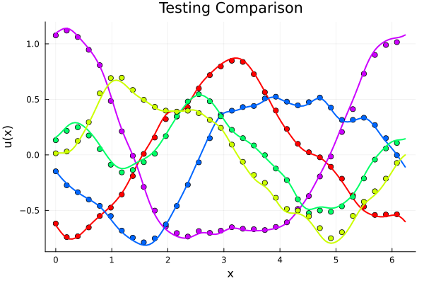
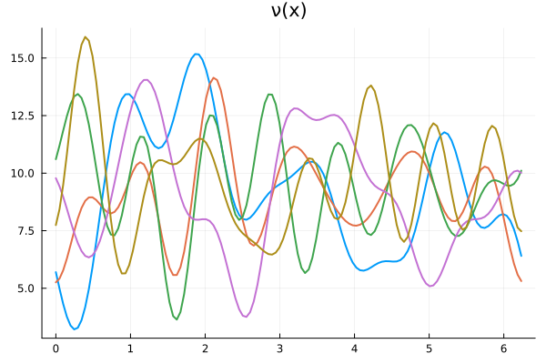
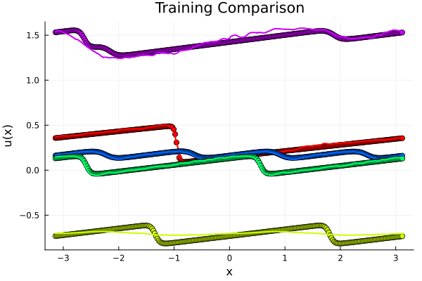
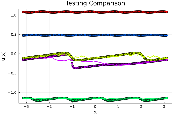
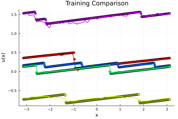
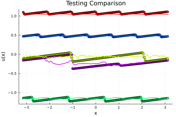
Experiment: Introduce random scales in test set by multiplying with envelop function \(e^{k\sin(\lambda x - \mu)} \)

Experiment: \(-\nabla \cdot \nu \nabla u = f\)

Modified FNO

Classic FNO

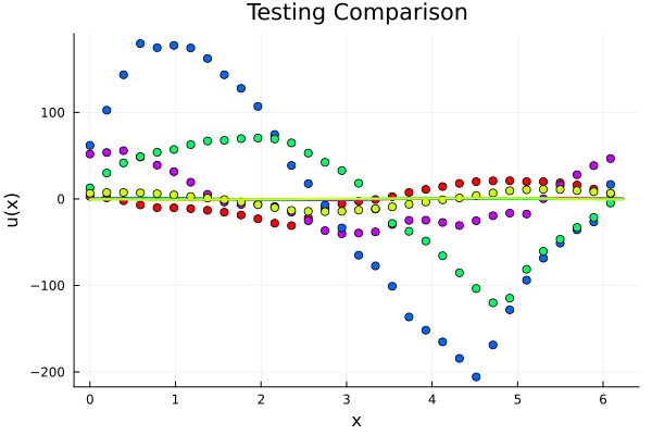
\(R^2=0.97\) on test set

\(R^2=0.002\) on test set

Experiment: \(-\nabla \cdot \nu \nabla u = f\)

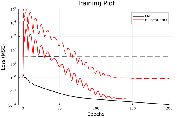
Solid line -> training set, Dashed line -> test set

Discussion

Modified architecture guarantees linearity in \(f\)
Training on \(\{f_i\}_{i=1}^K\), model learns solution for all \(\Sigma_{i=1}^K \alpha_i f_i \).
Optimal choice for \( f_i \): first \(K\) Fourier basis functions because they are orthonormal
Consider \( \mathrm{NN}(\nu, f) = \underline{\underline{\mathrm{NN}(\nu)}}\cdot f\) (matrix-vector product).
Then \(\underline{\underline{\mathrm{NN}(\nu)}}\) is a low rank approximation of inverse PDE operator with rank \(K\) (if \(f_i\) orthogonal).

\begin{cases} \mathrm{NN}(\nu, f_1) + \mathrm{NN}(\nu, f_2) = \mathrm{NN}(\nu, f_1 + f_2)\\ \mathrm{NN}(\nu, \lambda \cdot f) = \lambda \cdot \mathrm{NN}(\nu, f) \end{cases}

Disucssion

Superior generalizability with sparse data can be achieved by tuning architecture to PDE.
Question: To what extent are we interested in tuning architectures to specific PDEs?

Question: Should we write specialized models for other PDEs:
- Poisson, Helmholtz, Advection, etc
Question: What is the utility of low rank approximation to inverse operator? Need to lit review.

Next steps/ work in progress

To run 2D problems

Make code CUDA compatible - nearly done
Write a data-loader as GPUs have limited memory

To involve boundary conditions

Write Boundary Value Problem solver to generate data
Write backward ward pass for Discrete Cosine Transform (Chebyshev transform) - done
Write GPU compatible version of Discrete Cosine Transform

Weekly Meeting

AUG 4, 2023

Vedant Puri

https://github.com/vpuri3

Mechanical Engineering, Carnegie Mellon University

Advisors: Prof. Burak Kara, Prof. Jessica Zhang

Updates

\begin{cases} L_a(u) = f, & x\in\Omega\\ u|_{\partial\Omega} = g \end{cases}

Target Problem

Find (surrogate) map \( (x, a, f, g, \dotsc) \longrightarrow u \)

Efficient, generalizes with sparse data

So Far ( ~ 1/3 of the way there)

Neural Operator 1D/ 2D models
Benchmarks (1D advection, 2D Darcy flow, 1D/2D Poisson, 1D burgers)
Discussed parameter splitting idea for linear PDEs

Next Steps

Do validation in 2D
Involve Boundary Conditions

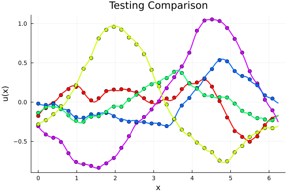
Validating FNO model: \((\partial_t - \partial_x) u = f\)

\(70k\) parameters
4x Operator Layers \( 32 \times 32\), \(16\) modes
Train/test \(R^2=0.998\), MSE \(10^{-3}\)

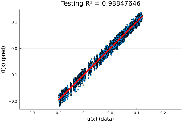
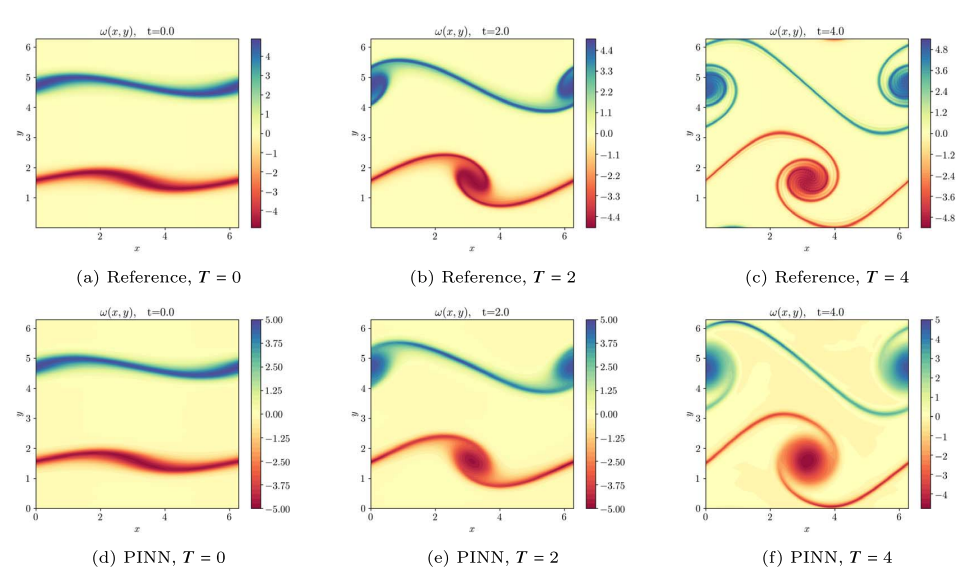
Validating FNO model: \(\partial_t + u\partial_x u = \nu\Delta u\), \( \nu = 10^{-2}\)

\(198k\) parameters, 6x Operator Layers \( 16 \times 16\), \(128\) modes

R² score: 0.9982961
MSE (mean SQR error): 0.00057452
RMSE (root mean SQR error): 0.02396922
MAE (mean ABS error): 0.01535009

R² score: 0.9795042
MSE (mean SQR error): 0.00701486
RMSE (root mean SQR error): 0.08375475
MAE (mean ABS error): 0.05496668

Validating FNO model: \(\partial_t + u\partial_x u = \nu\Delta u\), \( \nu = 10^{-2}\)

\(198k\) parameters, 6x Operator Layers \( 16 \times 16\), \(128\) modes

R² score: 0.9975712
MSE (mean SQR error): 0.00079163
RMSE (root mean SQR error): 0.02813594
MAE (mean ABS error): 0.01866633

R² score: 0.9755317
MSE (mean SQR error): 0.00802541
RMSE (root mean SQR error): 0.08958465
MAE (mean ABS error): 0.06163863

Involving Boundary Conditions

\begin{cases} L_a(u) = f, & x\in\Omega\\ u|_{\partial\Omega} = g \end{cases}

Why

Want to solve BVPs in changing geometries

TO DO

Utilize an isoparametric mapping to deform box mesh to generate geometries
Generate boundary value problem data in varying geometries
Extend Fourier Neural Operator to use Chebyshev transform
Test parameter splitting idea -------------------->

u = u_{\{a\},f_0} + u_\text{\{a\},\{g\}} + u_{\{a\},\{f\}}

\begin{cases} L_a(u) = f_0,\\ u|_{\partial\Omega} = 0 \end{cases}

\begin{cases} L_a(u) = 0,\\ u|_{\partial\Omega} = g \end{cases}

\begin{cases} L_a(u) = f-f_0,\\ u|_{\partial\Omega} = 0 \end{cases}

\(N_a\) samples

\(N_a\cdot N_g\) samples

\(N_a\cdot N_f\) samples

Weekly Meeting

AUG 16, 2023

Vedant Puri

https://github.com/vpuri3

Mechanical Engineering, Carnegie Mellon University

Advisors: Prof. Burak Kara, Prof. Jessica Zhang

Logistics: Classes

4/8 done (need 2 MechE courses + math req)
Classes (Fall 2023)
- 15-213: Introduction to Computer Systems (freshman level course - pre-req to most CS classes)
- 15-860: Monte Carlo Methods (taught by Keenan Crane)
- Would prefer to switch to: 24-703 (Prof. Zhang)/ 24-787 (Prof. Kara)

24-703: Numerical Methods in Engineering

24-787: Machine Learning and AI for Engineers

15-860: Monte Carlo Methods and Applications

15-513: Introduction to Computer Systesm

Logistics: Computer

Need to return laptop to Venkat before fall semester starts
Prof. Kara has offered to buy a laptop, Prof. Zhang, a desktop
Requirements: CPU (16+ cores) + GPU (12+ GB RAM)
Would prefer laptop as both labs have remote machines
If workstation/server is preferable, happy to buy my own laptop

Updates

\begin{cases} L_a(u) = f, & x\in\Omega\\ u|_{\partial\Omega} = g \end{cases}

Target Problem

Find surrogate map \(p = (x, a, f, g, \dotsc) \longrightarrow u \) for BVP

So Far

1D/ 2D Fourier Neural Operator with periodic BC, uniform grids

Earlier Proposal

Involve boundary conditions with convolutions over \( \partial\Omega\)
Extend to complex geometry with isoparametric mapping
Equation specific modifications (split training, bilinear layer)
Restricted to structured grids...

Literature Review

Extend to unstructured grids

Neural Operators and Green's functions

u({x}) = \int_\Omega G({x}; {y}) f({y}) \mathrm{d}y

L(G(x; y)) = \delta_{x, y}

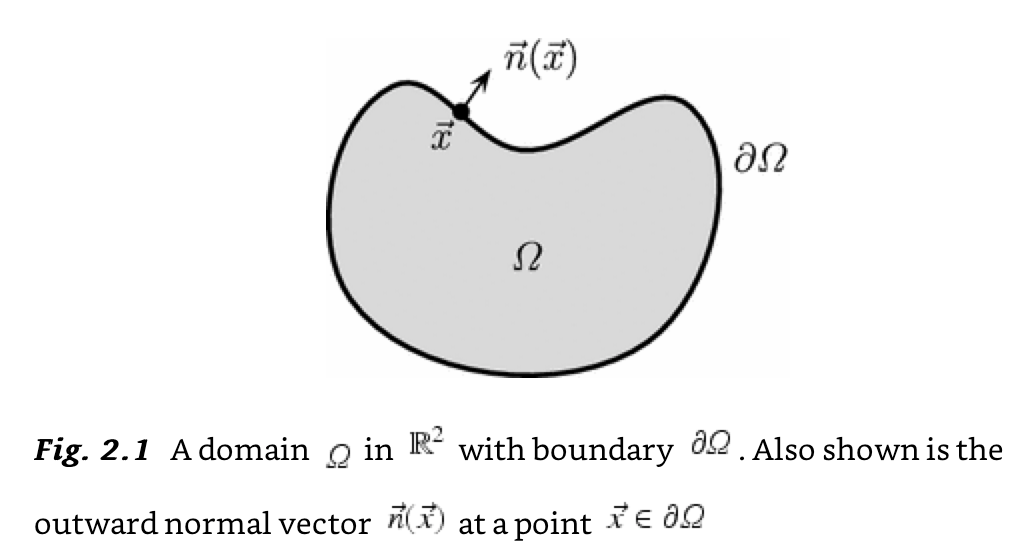
For PDE \( \mathcal{L}(u) = f, \, x \in \mathbb{R}^d \), the Green's function \(G(x; y)\) solves

Neural Operator models approximate the Green's function. Each layer performs the following operation

z_{l + 1} = \sigma \circ \left( W_{\theta}\cdot z_l + \int_{\mathbb{R}^d} \mathcal{K}_{\theta}(z_l; y) \mathrm{d}y \right)

Eg, the Fourier Neural Operator

z_{l + 1} = \sigma \circ \left( W_{1,\theta}\cdot z_l + \mathcal{F}^{-1}( W_{2,\theta}\cdot\mathcal{F}(z_l)) \right)

where \(\mathcal{F}\) is the Fourier transform

\mathcal{F}(z_1)\odot\mathcal{F}(z_2) = \mathcal{F}(z_1 \ast z_2)

Neural Operators are grid independent

G^{6}

G^{3}

\begin{pmatrix} \widehat{u_1}^3\\ \widehat{u_2}^3\\ \widehat{u_3}^3\\ 0\\ 0\\ 0\\ \end{pmatrix} = \underbrace{ \begin{bmatrix} 1 & 0 & 0\\ 0 & 1 & 0\\ 0 & 0 & 1\\ 0 & 0 & 0\\ 0 & 0 & 0\\ 0 & 0 & 0\\ \end{bmatrix} }_{J_{6, 3}} \begin{pmatrix} \widehat{u_1}^3\\ \widehat{u_2}^3\\ \widehat{u_3}^3\\ \end{pmatrix}

\(G^6 \leftarrow G^3 \) interpolation

Neural Operators parameterize the model in a latent space that can be interpolated to any grid

u_6 = \mathcal{F}_6^{-1} \circ J_{6, 3} \circ \mathcal{F}_3(u_3)

u = \mathcal{F}^{-1} \circ \mathrm{NN}_\theta \circ \mathcal{F} (p)

Spectral Neural Operator is an architecture that learns a model in spectral space

Spectral expansion and transform

u(x) = \sum_{n} \widehat{u}_n\phi_n(x)

orthonormal basis

transform matrix

\underline{u} = \sum_{n=1}^N \widehat{\underline{u}}_n\phi_n(x) = \underbrace{ \begin{bmatrix} \underline{\phi}_1 & \underline{\phi}_2 & \cdots & \underline{\phi}_N & \end{bmatrix}_{N \times N} }_{\mathcal{F}^{-1}} \begin{pmatrix} \widehat{u_1}\\ \widehat{u_2}\\ \vdots\\ \widehat{u_N}\\ \end{pmatrix}_{N \times 1} = \mathcal{F}^{-1}(\widehat{u})

\mathcal{F}^{-1} = [\Phi_n(x_m)]_{m, n} , \,\, \mathcal{F} = [\Phi_m(x_n)]_{m, n}

\underline{u}(x_m) = \sum_n \phi_n(x_m) \widehat{\underline{u}}_n ,\,\, \widehat{\underline{u}}_m = \sum_n \phi_m(x_n) \underline{u}_n

Spectral expansion and transform

\langle \phi_m, \phi_n \rangle = \int_a^b \phi_m(x) \phi_n(x) \underbrace{w(x) \mathrm{d}x}_{\mathrm{d}\alpha}

Orthogonal WRT inner product on \( C(\mathbb{R}) \)

(Classical Orthogonal Polynomials)

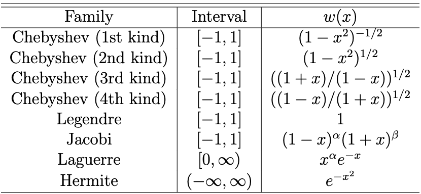
On \(S_1 = \{|z| =1, \, z \in \mathbb{C} \} \) (Fourier) and weight \( w(z) = 1\), we get \( \exp{(ikx)}, \, k\in\mathbb{N}\) on interval \( [0, 2\pi) \)

Many properties (Sturm-Louisville, convolution...)

Proposed model with boundary convolutions

\begin{cases} L(u) = f, & x\in\Omega\\ u|_{\partial\Omega} = g \end{cases}

Based on Green's function solution to BVP

u({x}) = \int_\Omega G_\Omega({x}; {y}) f({y}) \mathrm{d}y + \int_{\partial\Omega} G_{\partial\Omega}({r}; {s}) g({s}) \mathrm{d}s

u(x) = \int_\Omega G(x, y) f(y) d y + \int_{\partial\Omega} \nabla \cdot G(x, y) g(y) d y

Eg, Poisson equation, \(L(u) = \Delta u \)

Proposed model layers involve boundary information with convolutions

z_{l + 1} = \sigma \circ \left( W_{1,\theta}\cdot z_l + \mathcal{F}_{\Omega}^{-1}( W_{2,\theta}\cdot\mathcal{F}_{\Omega}(z_l)) + \mathcal{F}_{\partial\Omega}^{-1}( W_{3,\theta}\cdot\mathcal{F}_{\partial\Omega}(z_l)) \right)

Model can train on multiple geometries (generated by deforming a fixed spectral patch)

Neural Operators on Unstructured Grids

Spectral expansions are defined on simple grids (boxes, triangles, circles, tensor products) and deformations. Challenge is to find a spectral expansion on general meshes.

\mathcal{F}^{-1} = [\Phi_n(x_m)]_{m, n} = \begin{bmatrix} \underline{\phi}_1 & \cdots & \underline{\phi}_K \end{bmatrix}_{N \times K}

One approach is to preselect a basis. For a meshed domain, \( \Omega\), precompute the first \(K\) eigenfunctions of the Laplacian, \( \Delta \phi = \lambda \phi \)

u = \mathcal{F}^{-1} \circ \mathrm{NN}_\theta \circ \mathcal{F} (p)

Then, employ the Spectral Neural Operator model (Laplace Neural Operator)

This model is resolution independent, as the eigenfunctions can be interpolated to any mesh, but does not generalize to new geometries.

Learn a spectral transformation on a general grid
- At the end of the day, the transform is just an invertible operation
- For FNO, it is simply a matrix
- Can we learn an invertible operation and use it in the operator layers?
Implicit Neural Representations (INRs) for operator learning
- INRs can be used to learn mappings from a general geometry to a latent space
- INRs model input as output of an implicit function \( p = \mathrm{NN}_\theta(x) \)
- Two step process:
  - learn forward/backward mapping - utilize
  - train deep neural network in latent space

Neural Operators on Unstructured Grids

Weekly Meeting

SEP 11, 2023

Vedant Puri

https://github.com/vpuri3

Mechanical Engineering, Carnegie Mellon University

Advisors: Prof. Burak Kara, Prof. Jessica Zhang

Overview

\begin{cases} L_a(u) = f, & x\in\Omega\\ u|_{\partial\Omega} = g \end{cases}

Target Problem:

Find (surrogate) map \( (x, a, f, g, \dotsc)\longrightarrow u \)
in complex geometries, with varying boundary conditions

Work Done till Now

Implemented neural operator models
Literature review

Talking to

Aviral Prakash, post-doc w. Prof. Zhang
- works on turbulence reduced order modeling
Kevin Ferguson, PhD student w. Prof. Kara
- works on surrogates on meshes

Landscape of ML for PDEs

Mesh-based

PDE-Based

Neural Ansatz

Data-driven

FEM, FVM, IGA, Spectral

Fourier Neural Operator

Implicit Neural Representations

DeepONet

Physics Informed NNs

Convolution NNs

Graph NNs

Adapted from Núñez, CEMRACS 2023

Deep Galerkin

Neural ODEs

Universal Diff Eq

Hybrid Phys/ML

Landscape of ML for PDEs

Mesh-based

PDE-Based

Neural Ansatz

Data-driven

FEM, FVM, IGA, Spectral

Fourier Neural Operator

Implicit Neural Representations

DeepONet

Physics Informed NNs

Convolution NNs

Graph NNs

Adapted from Núñez, CEMRACS 2023

Deep Galerkin

Neural ODEs

Universal Diff Eq

Hybrid Phys/ML

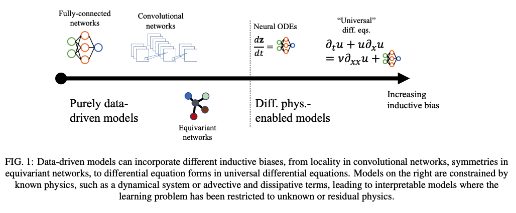
Universal Differential Equations

Motivation

Learning requires large data, unavailable in scientific domains
Data in physics models is available in form of differential equations
PDE models extrapolate better than purely learned surrogates

Mix ML with PDE solvers:

Involve PDE biases in ML model \(\iff\) learn unknown PDE params with ML

Application

Learn correction to physics simulation with data (eg closure modeling)
Closure modeling, reduced order modeling

Universal Differential Equations

Universal Diff Eq Example: Closure Modeling

\partial_t \bar{u} + \bar{u} \partial_x \bar{u} = \nu \partial_x ^2 \bar{u} + \eta

Closure Model

\eta := \text{NN}_\theta(u)

Eddy Viscosity Model

Vanilla Neural Network

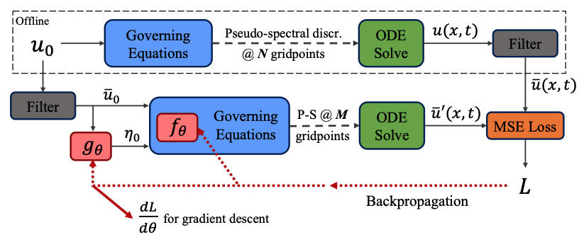
\partial_t\nu_T + \alpha_\theta(\bar{u}\partial_x \nu_T) = \beta_(\theta\nu\partial_{xx}\nu_T)

\eta := \partial_x(\nu_T\partial_x\bar{u})

The algorithmic backbone of this method is the interpolating adjoint method for backpropagating through ODE solve

UDEs need ML to the simulation pipeline

Mesh

\(A\underline{u} = M\underline{f} \)

Domain

Governing Equation

Boundary Constraint

\( NN_\theta \)

Discretization

\( \dfrac{d}{dt} \underline{u} = f(\underline{u}) \)

Solving

Discrete Problems

\(u(\underline{x},t) \)

\(u(\underline{x}) \)

Solution

Loss

Backpropogation

Data

\( NN_\theta \)

Linear Solver

Time-Stepper

Landscape of ML for PDEs

Mesh-based

PDE-Based

Neural Ansatz

Data-driven

FEM, FVM, IGA, Spectral

Fourier Neural Operator

Implicit Neural Representations

DeepONet

Physics Informed NNs

Convolution NNs

Graph NNs

Adapted from Núñez, CEMRACS 2023

Deep Galerkin

Neural ODEs

Universal Diff Eq

Hybrid Phys/ML

PINNs: Physics Informed Neural Networks

Replace PDE solver with a neural network
Automated PDE solving - just need to type in equation
No data gen, no solver, no mesh
Just set up model and run

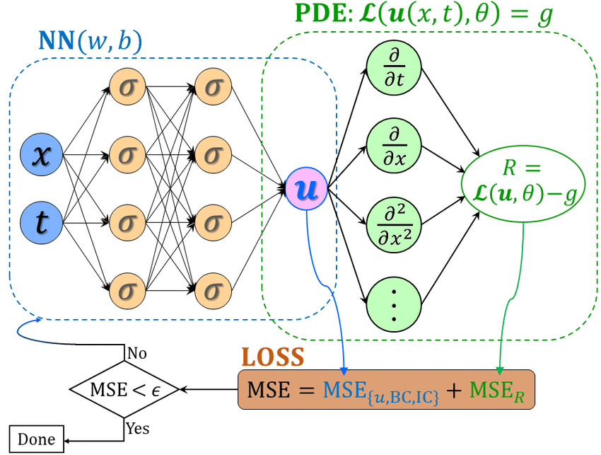
PINNs: Physics Informed Neural Networks

Replace PDE solver with a neural network
\( u = \mathrm{NN}_\theta(x, t)\) (neural ansatz)
Overfit a network to PDE by minimizing
Trained by minimizing PDE residual (LHS-RHS) at sample points
- Kind of like collocation on (randomly) select points in domain
Residual computed via automatic differentiation (exact)

PINNs: Physics Informed Neural Networks

Advantages

Automated methodology, no prior data required
If data available, just add it to loss function!
Small networks are able to do a good job
In principle, mesh free. Need domain points for discretizing loss function but no topology required

PINNs: Physics Informed Neural Networks

Challenges

Struggle with large/complex domains, multiscale solutions. Both require many sample points
Need extra sampling at boundaries to enforce BC
Hard to train (loss landscape depends on PDE, \(\lambda_i\), IC/BC add constraints to optimization problem)

L(u, \theta) = L_\text{phys}(u, \theta) + \lambda_1 \cdot L_\text{BC}(u, \theta) +\\ \lambda_2 \cdot L_\text{IC}(u, \theta) + \lambda_3 \cdot L_\text{data}(u, \theta)

\frac{du}{dx} = cos(1 x)

PINNs: Physics Informed Neural Networks

Many variants out there

HyperPINNs: Mixing PINNs with hyper networks
BayesianPINNs: estimate uncertainty in PDE solution
Deep Ritz/ Deep Galerkin: Minimize Galerkin residual in place of collocation
Use convolution/ graph network architecture to minimize physics loss
XPINN: (domain decomposition approach) train separate PINNs in subdomains
In principle, physics loss can be included in any ML model

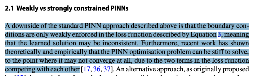
However, key problems persist

Soft imposition of IC/BC via loss function lead to insufficient accuracy, unnecessary training effort
Hard to train

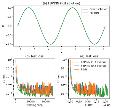
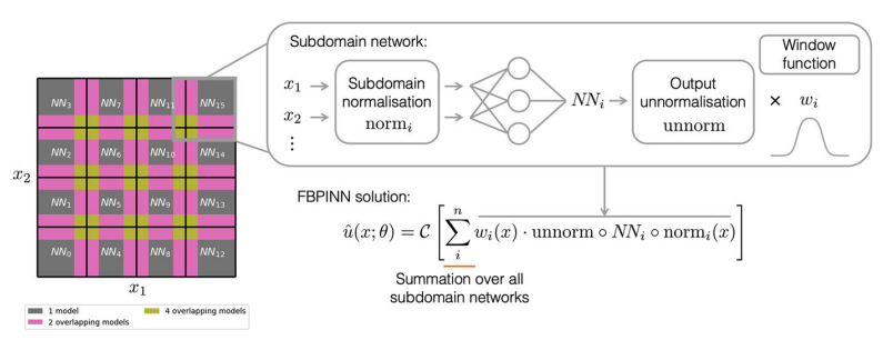
PINNs: Domain Decomposition

Finite Basis PINNs, 2023

\frac{du}{dx} = cos(15 x)

PINNs: Multi-stage Training

Divide training into stages
- Train model on data
- \(\longrightarrow\) train new model to capture error
- \(\longrightarrow\) repeat
Incremental networks capture higher frequency modes
Kind of like multigrid method

Jul 2023

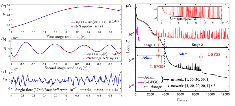
PINNs: Multi-stage Training

Landscape of ML for PDEs

Mesh-based

PDE-Based

Neural Ansatz

Data-driven

FEM, FVM, IGA, Spectral

Fourier Neural Operator

Implicit Neural Representations

DeepONet

Physics Informed NNs

Convolution NNs

Graph NNs

Adapted from Núñez, CEMRACS 2023

Deep Galerkin

Neural ODEs

Universal Diff Eq

Hybrid Phys/ML

Landscape of ML for PDEs

Mesh-based

PDE-Based

Neural Ansatz

Data-driven

FEM, FVM, IGA, Spectral

Fourier Neural Operator

Implicit Neural Representations

DeepONet

Physics Informed NNs

Convolution NNs

Graph NNs

Adapted from Núñez, CEMRACS 2023

Neural ODEs

Universal Diff Eq

u =

\dfrac{du}{dt} =

\dfrac{d\tilde{u}}{dt} = \tilde{\mathcal{L}}_p(\tilde{u}) +

\dfrac{du}{dt} = \mathcal{L}_p(u) + \mathcal{N}_p(u)

\begin{cases} \dfrac{d u}{dt} = \mathcal{L}_p(u) + \mathcal{N}_p(u), & x\in\Omega\\ u|_{\partial\Omega} = g(t) \end{cases}

Weekly Meeting

SEP 14, 2023

Vedant Puri

https://github.com/vpuri3

Mechanical Engineering, Carnegie Mellon University

Advisors: Prof. Burak Kara, Prof. Jessica Zhang

Landscape of ML for PDEs

Mesh-based

PDE-Based

Neural Ansatz

Data-driven

FEM, FVM, IGA, Spectral

Fourier Neural Operator

Implicit Neural Representations

DeepONet

Physics Informed NNs

Convolution NNs

Graph NNs

Adapted from Núñez, CEMRACS 2023

Neural ODEs

Universal Diff Eq

Hybrid Phys/ML

u =

\dfrac{du}{dt} =

\dfrac{d\tilde{u}}{dt} = \tilde{\mathcal{L}}_p(\tilde{u}) +

\dfrac{du}{dt} = \mathcal{L}_p(u) + \mathcal{N}_p(u)

\begin{cases} \dfrac{d u}{dt} = \mathcal{L}_p(u) + \mathcal{N}_p(u), & x\in\Omega\\ u|_{\partial\Omega} = g(t) \end{cases}

Generative Models??

Landscape of ML for PDEs

Model	Target Problem	Methodology/ Limitation	Input/ Output
UDE	Learn unknown physics from data	Differentiate through PDE solve to learn unknown params FWD pass: solve PDE w. FEM/spectral with added NN term BWD pass: (adjoint method) run sim in reverse to get sensitivities	Learn to match with data by solving
PINN	Replace solver with black-box NN	(Non-parametric model) learn PDE solution for fixed parameters p by overfitting NN with PDE residual + IC/BC loss + data. Very hard to train.	Evaluate at sampled points in
CNN/GNN	Learn parametric from mesh data	Utilize domain mesh/grid structure to learn sparse convolutions. Grid-to-grid model. Limited to predicting on training grid.	Evaluate on grid
FNO	Learn parametric solution operator for PDE from data + PDE loss	Learn params in Fourier space (resolution independent). Architecture: pointwise evals + global convs. Function-to-function model, but limited to uniform grids	Evaluate on uniform grid of any res.
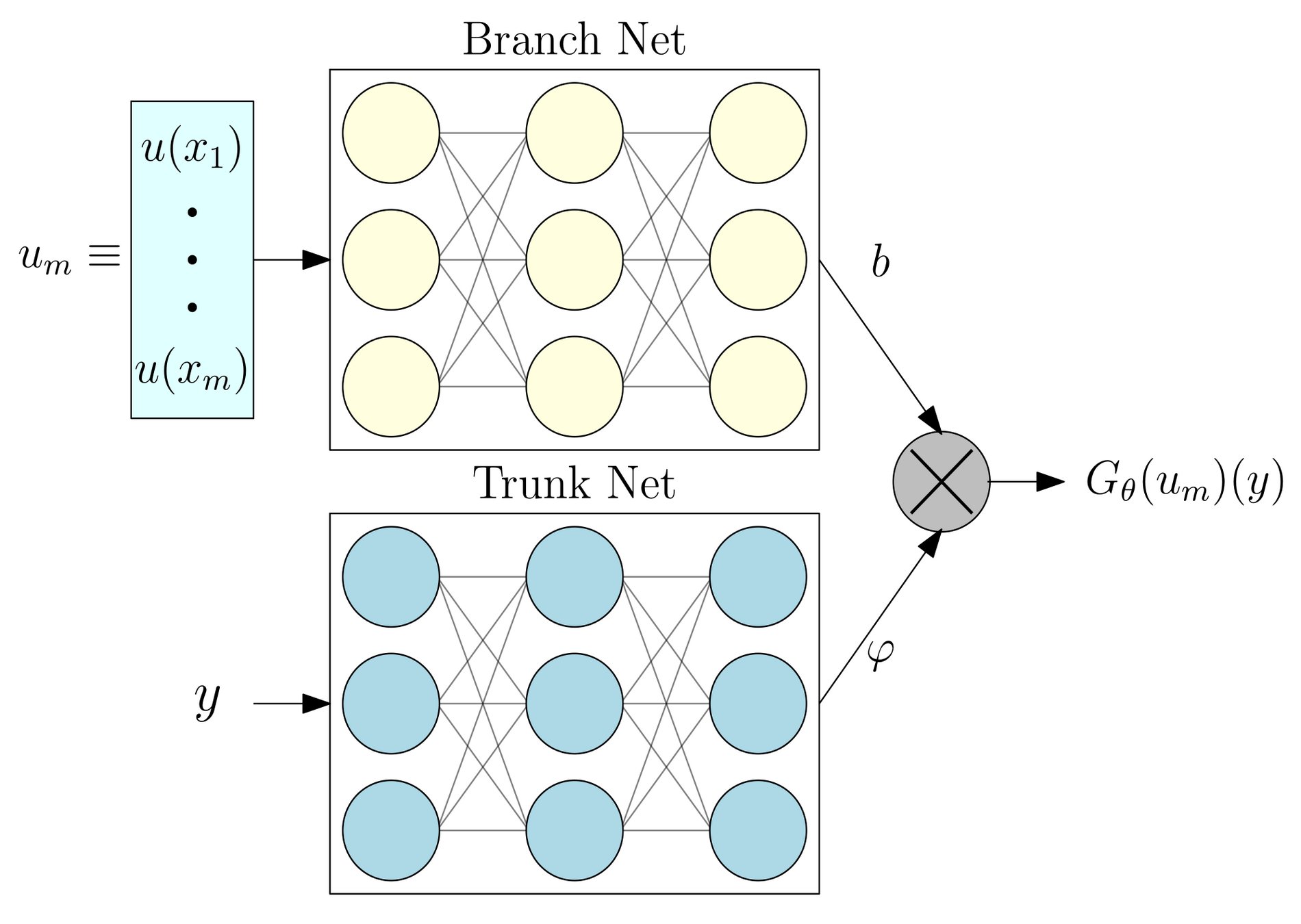
DeepONet	Learn parametric over from fixed sensors locations. Loss PDE + data	Mimics PDE solve in NN. Linear combination of - learned basis functions spanning from fixed sensor points - learned scaling coefficients for basis Function-to-function model	For fixed sensor points and arbitrary ,

\begin{cases} \mathcal{L}_p(u) = 0, & x\in\Omega\\ u|_{\partial\Omega} = g \end{cases}

\tilde{\mathcal{L}}_{p, \theta}(\tilde{u}) = 0

u = \mathrm{NN}_\theta(x)

\Omega

\forall y \in\Omega

\{x_i\}

y\in\Omega

u(y) = \mathrm{NN}_\theta(y, p|_{\{x_i\}})

\Omega

u(\cdot; p)

u|_{G^h} = \mathrm{NN}_\theta(p|_{G^h})

G^h

\theta

u(\cdot; p, \theta)

u|_{G^h} = \mathrm{NN}_\theta(p|_{G^h})

\theta

Operator learning: continuous analog of supervised learning

\(\implies\) can evaluate anywhere in \(\Omega\)
\(\implies\) prediction quality grid independent
\(\implies\) discretization convergent

FNO vs CNN

Both are grid-to-grid model

Fourier transform / convolution equivalent (conv. theorem). For signal \(f\), filter \(g\)

Input

\( C_{i} \times Nx \times Ny\)

Model

Output

\( C_{o} \times Nx \times Ny\)

\mathcal{F}(f) \odot \mathcal{F}(g) = \mathcal{F}(f \ast g)

CNN learns local (\(2\times2\)) filter \(g\)
FNO learns \( 32 \times 32\) filter freqs, \(\mathcal{F}(g)\).
- Filter is local in Fourier space \(\iff\) global in mode space
- Global filter implemented with FFT (doesn't care about resolution)

FNO vs Convolution Networks

	Fourier Neural Operator	Convolution Neural Network
Target problem	Function-to-function mapping	Grid-to-grid mapping
Methodology	- Pointwise ops (MLP/ 1x1 conv) capture local features - Global convolutions capture global info (learned in Fourier space)	Learn local convolution filters
Continuity	Input/output continuous function (can be evaluated anywhere) In practice, sampled on uniform grids.	Input/output are data on uniform grids
Resolution dependence	Performance comparable when evaluated on finer grids.	Performance degrades on finer/coarser grids than training grid.
Evaluate on finer grids	Can evaluate on any grid High-frequency features (not present on training grid) can be captured.	Downsample --> evaluate --> Interpolate Loses high-frequency features

DeepONet

FNO vs DeepONet

	Fourier Neural Operator	DeepONet
Target problem	Function-to-function mapping	Function-to-function mapping
Methodology
Continuity
Interpolation
Resolution dependence

FNO vs Convolution Networks

Differences

FNO is a continuous model, CNN discrete
FNO can be evaluated on uniform grids of any resolution (in principle)
FNO learns model in Fourier space
Every layer has FFT which is global operation (like transformer)
Inverse Fourier transform adds Fourier features to every layer
CNN can be evaluated on denser grids but only with subsampling
CNN performance degrades on different resolutions

Lifting Op

Linear transform on first \(K\) Fourier modes

Local linear transform

Projection Op

FNO Working

#==============================#
# Lifting
v [Cv, Nx, Ny] <- P [Cp, Ca] * a [Ca, Nx, Ny]

#==============================#
# Fourier layer

## local
w1 [Cw, Nx, Ny] <- W_loc [Cw, Cv] * v [Cv, Nx, Ny]

## modal
vh [Cv, Kx, Ky] <- FFT   * v [Cv, Nx, Ny] # Transform
vh [Cv, Mx, My] <- Trunc * vh[Cv, Kx, Ky] # Truncation

wh [Cw, Mx, My] <- R [Cw, Cv, Mx, My] * vh [Cv, Mx, My]

wh [Cw, Kx, Ky] <- ZeroPad * wh [Cw, Mx, My] # Zero Pad
w2 [Cw, Nx, Ny] <- iFFT    * v  [Cv, Kx, Ky] # iTransform

w = w1 + w2

#==============================#
# Projection
u [Cu, Nx, Ny, B] <- Q [Cu, Cw] * a [Cw, Nx, Ny, B]

Lifting Op

Linear transform on first \(K\) Fourier modes

Local linear transform

Projection Op

# Modal operation in Fourier Layer

wh [Cw, Mx, My] <- R [Cw, Cv, Mx, My] * vh [Cv, Mx, My]

## in index notation:
wh[cw, mx, my] <- W_mod [cw, cv, mx, my] * vh [cv, mx, my]

# contraction in cv
# elementwise mult in mx, my

Updates 9/18/23

Discussions on Neural Operator (w. Prof. Kara)
- Figure out what is novel in architecture (by comparison with CNNs)
- Find areas of improvement/ new application
Possible applications
- PDE solvers for complex geometry, changing boundary conditions
Reduced Order Modeling (w. Aviral)
- Use ML models for dimensionality reduction in fluid flow problems
- Current approaches use autoencoders, neural fields
- Can we involve operator models?

Paper snapshot (title + authors). What does it claim to do?
Methodology: how does it do it?
Novelty: what is novel? methodology? use case?
Future directions?

Advisor Meeting

Agenda

Motivation: close the loop in Computer-Aided-Engineering Cycle

Geometry discretization is a major bottleneck

Want: solve PDEs in complex geometries

Topic - machine learning accelerated meshing

Topic - machine learning accelerated meshing

Topic - machine learning based PDE surrogates

Aside - ML beats the Curse of Dimensionality-ish

Aside - our goal is to add ML to the simulation pipeline

Aside - We are building an differentiable PDEs ecosystem

PDE Surrogates - Learning the closure to Burgers turbulence

PDE Surrogates - machine learning has an I/O problem

PDE Surrogates - convolutions

PDE Surrogates - we take inspiration from finite-element method

Topic - isogeometric analysis

Advisor Meeting

Geometry Operator Learning

Geometry Operator Learning

Discussion

Sandbox: start with 1D Fourier method

In 2D

Advisor Meeting

Geometry Operator Learning

Experiment 1 - diagonal system

Experiment 1 - diagonal system

Experiment 2 - 1D Fourier Collocation

Experiment 2 - 1D Fourier

Weekly Meeting

Updates - Geometry Operator Lerning

Updates

Weekly Meeting

From last week (5/26/23)

From last week (5/26/23)

Updates

Geometry Operator Learning - Lit Review

Updates

Weekly Meeting

References

Problem Setting

Conventional approach: discretize then learn

Neural operators map between Banach spaces

Neural operator models

PCA-NET

DEEPONET

Aside: Green's function and integral operators

Operator models approximate Green's function

Graph Kernel Network

Using a spectral fourier basis has advantages

Fourier neural operator

Fourier neural operator results

Advantages

Discussion

Use-Cases

Discussion

Disadvantages

Ideas - how to proceed further?

Weekly Meeting

Updates

Neural Operators

Neural Operators

Neural Operator Capabilities/ limitations

Our Goals

Neural Operators Methodology

Fourier Neural Operator

Involve BC in Neural Operators

Proposed Methodology

Weekly Meeting

Updates

Experiment

Experiment Part I

Experiment Part II (WIP)

Updates

Proposed Methodology

Weekly Meeting

Updates

Neural Operator Kernel

Experiment

Experiment I: \(-\nabla \cdot \nu_0 \nabla u = f \)

Experiment I: \(-\nabla \cdot \nu_0 \nabla u = f \)