Learning From Corrupt/Noisy Data
July 1, 2025
Adam Wei
Agenda
- Review of Ambient Diffusion
- Experiments & Results
- [Time Permitting]: Next directions
Part 1
Ambient-Omni
Corrupt Data
Corrupt Data (\(q_0\))
Clean Data (\(p_0\))
Computer Vision
Language


Poor writing, profanity, toxcity, grammar/spelling errors, etc


👀
Sources of Robot Data
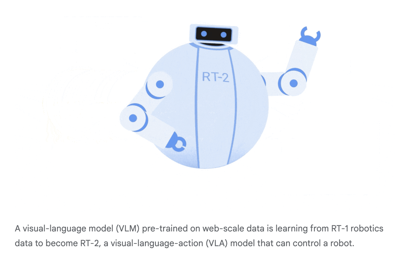
Open-X
expert robot teleop
robot teleop
simulation

Goal: sample "high-quality" trajectories for your task
Train on entire spectrum to learn "high-level" reasoning, semantics, etc
"corrupt"
"clean"
Research Questions
- How can we learn from both clean and corrupt data?
- Can these algorithms be adapted for robotics?

Giannis Daras
Research Questions
Giannis Daras
Ambient Diffusion
Three key ideas
1. Corrupt data points should be contracted (masked with noise) and used at higher noise levels
2. Ambient loss function
3. OOD data with locality can be used at lower noise levels
Ambient Diffusion: 1 and 2
Ambient-o Diffusion: 1, 2, and 3
1. Learning in the high-noise regime
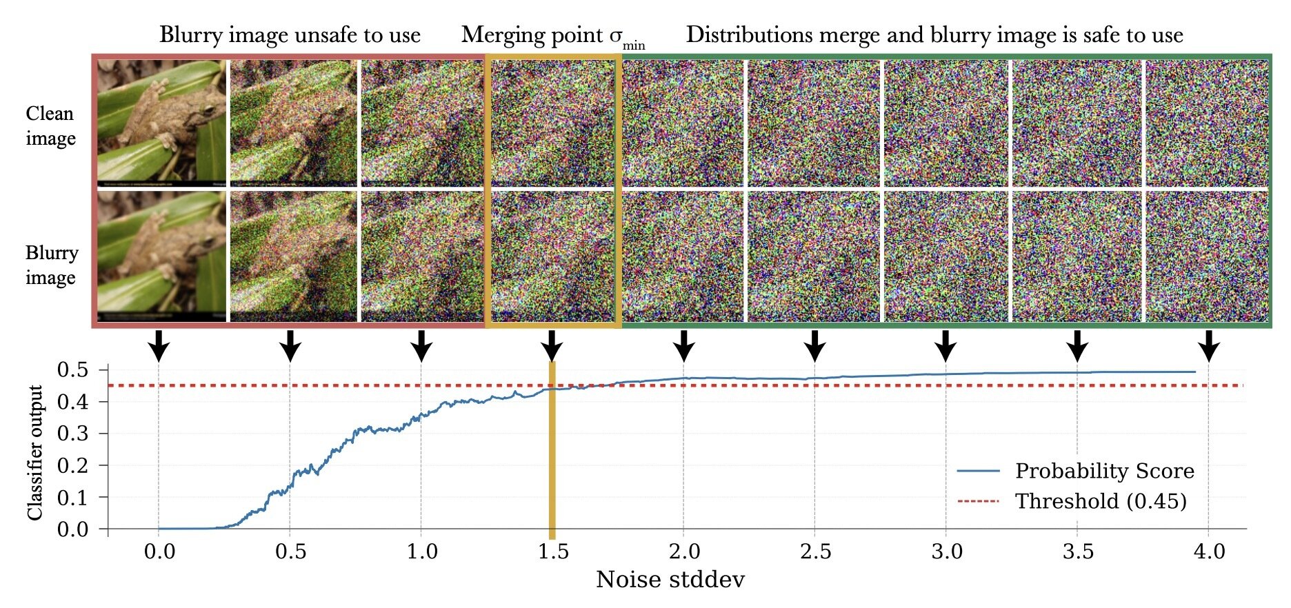
\(\exists \sigma_{min}\) s.t. \(d_\mathrm{TV}(p_{\sigma_{min}}, q_{\sigma_{min}}) < \epsilon\)
(in this example, \(\epsilon = 0.05\))
\(p_0\)
\(q_0\)
1. Learning in the high-noise regime
\(\exists \sigma_{min}\) s.t. \(d_\mathrm{TV}(p_{\sigma_{min}}, q_{\sigma_{min}}) < \epsilon\)
- Only use samples from \(q_0\) to train denoisers with \(\sigma > \sigma_{min}\)
- Corruption level of each datapoint determines its utility
\(\sigma=1\)
\(\sigma=0\)
\(\sigma=\sigma_{min}\)
Clean Data
Corrupt Data
Contraction as masking
- Contracting \(q_{\sigma_{min}}\) towards \(p_{\sigma_{min}}\) "masks" corruption between \(p_0\) and \(q_0\)
... but also destroys useful signal
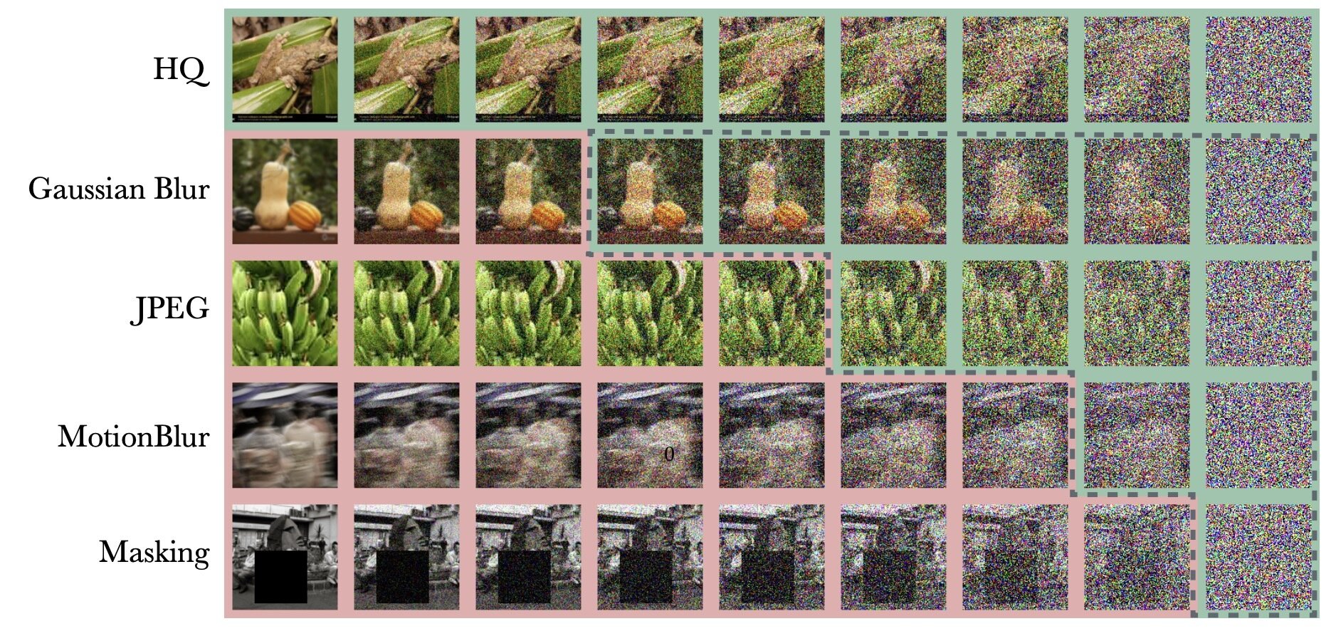
More info lost
Contraction introduces bias
\(q_\sigma \approx p_\sigma\) for \(\sigma > \sigma_{min}\), but not equal
Theoretical Analysis
Provided that
\(\implies\) training with \(q_0\) introduces bias!
Then \(\exists \sigma_{min} < 1\) s.t. learning from clean and corrupt data outperforms learning from clean only*
* as measured by TV between the learned \(\hat p\) and \(p_0\)
- \(p_0\) and \(q_0\) are reasonably similar
- Number of samples from \(q_0\) is large compared to \(p_0\)
- ... other mild conditions
2. Ambient Loss
\(\sigma=1\)
\(\sigma=0\)
\(\sigma=\sigma_{min}\)
Clean Data
Corrupt Data
Without Ambient Loss
\(\sigma=1\)
\(\sigma=0\)
\(\sigma=\sigma_{min}\)
\(\mathbb E[\lVert h_\theta(x_t, t) - x_0 \rVert_2^2]\)
\(\mathbb E[\lVert h_\theta(y_t, t) - y_0 \rVert_2^2]\)
Clean Data: \(x_0\)-prediction or \(\epsilon\)-prediction
Corrupt Data: \(x_0\) or \(\epsilon\)-prediction
\( x_0 \sim p_0\)
\( y_0 \sim q_0\)
Ambient Loss
\(\sigma=1\)
\(\sigma=0\)
\(\sigma=\sigma_{min}\)
\(\mathbb E[\lVert h_\theta(x_t, t) - x_0 \rVert_2^2]\)
\(\mathbb E[\lVert h_\theta(y_t, t) + \frac{\sigma_{min}^2\sqrt{1-\sigma_{t}^2}}{\sigma_t^2-\sigma_{min}^2}y_{t} - \frac{\sigma_{t}^2\sqrt{1-\sigma_{min}^2}}{\sigma_t^2-\sigma_{min}^2} y_{t_{min}} \rVert_2^2]\)
Corrupt Data: ambient loss*
\( x_0 \sim p_0\)
\( y_0 \sim q_0\)
* Giannis and I are working on the \(\epsilon\)-prediction versions
Clean Data: \(x_0\)-prediction or \(\epsilon\)-prediction
Ambient Loss
\(\sigma=1\)
\(\sigma=0\)
\(\mathbb E[\lVert h_\theta(x_t, t) - x_0 \rVert_2^2]\)
Corrupt Data: ambient loss*
\( x_0 \sim p_0\)
\( y_0 \sim q_0\)
* Giannis and I are working on the \(\epsilon\)-prediction versions
\(\sigma=\sigma_{min}\)
\(\sigma_{buffer}(\sigma_{min}, \sigma_t)\)
\(\mathbb E[\lVert h_\theta(y_t, t) + \frac{\sigma_{min}^2\sqrt{1-\sigma_{t}^2}}{\sigma_t^2-\sigma_{min}^2}y_{t} - \frac{\sigma_{t}^2\sqrt{1-\sigma_{min}^2}}{\sigma_t^2-\sigma_{min}^2} y_{t_{min}} \rVert_2^2]\)
Clean Data: \(x_0\)-prediction or \(\epsilon\)-prediction
Training Implementation Details
\(\sigma=1\)
\(\sigma=0\)
\(\mathbb E[\lVert h_\theta(x_t, t) - x_0 \rVert_2^2]\)
\( x_0 \sim p_0\)
\( y_0 \sim q_0\)
\(\sigma=\sigma_{min}\)
\(\sigma_{buffer}(\sigma_{min}, \sigma_t)\)
\(\mathbb E[\lVert h_\theta(y_t, t) + \frac{\sigma_{min}^2\sqrt{1-\sigma_{t}^2}}{\sigma_t^2-\sigma_{min}^2}y_{t} - \frac{\sigma_{t}^2\sqrt{1-\sigma_{min}^2}}{\sigma_t^2-\sigma_{min}^2} y_{t_{min}} \rVert_2^2]\)
- Dataloader: sample noise uniformly, then sample a datapoint
- Some other details... see paper
3. Learning in the low-noise regime
Ambient-o also presents a way to use OOD data to train denoisers in the low-noise regime
... future direction to try
- Ex. Training a dog generator with images of cats
Part 2
Experiments
Three key ideas -- tried two so far...
Experiments
1. Corrupt data points should be contracted (masked with noise) and used at higher noise levels
2. Ambient loss function
3. OOD data with locality can be used at lower noise levels
Experiments
Denoising Loss
Idea 2: Ambient Loss
* This is equivalent to:
Use corrupt data \(\forall \sigma\)
Idea 1: Use corrupt data \(\forall \sigma > \sigma_{min}\)
N/A
(reduces to baseline)
\(\epsilon\)-prediction*
\(x_0\)-prediction*
\(\epsilon\)-prediction
\(x_0\)-prediction
\(\epsilon\)-prediction**
\(x_0\)-prediction
** Giannis and I are working on the \(\epsilon\)-prediction ambient loss
- cotraining with no reweighting
- setting \(\sigma_{min} = 0\)
\(\sigma_{min}\)
- Find \(\sigma_{min}\) by training a classifier
- Can be assigned \(\sigma_{min}\) per-dataset or per-datapoint
In my experiments, I sweep \(\sigma_{min}\) at the dataset level
\(\sigma_{min}\in \{0.09, 0.16, 0.32, 0.48, 0.59, 0.81\}\)
Datasets and Task
"Clean" Data
"Corrupt" Data
\(|\mathcal{D}_T|=50\)
\(|\mathcal{D}_S|=2000, 4000, 8000\)
Eval criteria: Success rate for planar pushing across 200 randomized trials
Results
Experiments
Choosing \(\sigma_{min}\): Swept several values on the dataset level
Loss function: Tried all 4 combinations of
{\(x_0\)-prediction, \(\epsilon\)-prediction} x {denoising, ambient}
Preliminary Observations
(will present best results on next slide)
- \(\epsilon\)-prediction > \(x_0\)-prediction and denosing > ambient loss
- Small (but non-zero) \(\sigma_{min}\) performed best
- Ambient diffusion scales slightly better with more sim data than cotraining
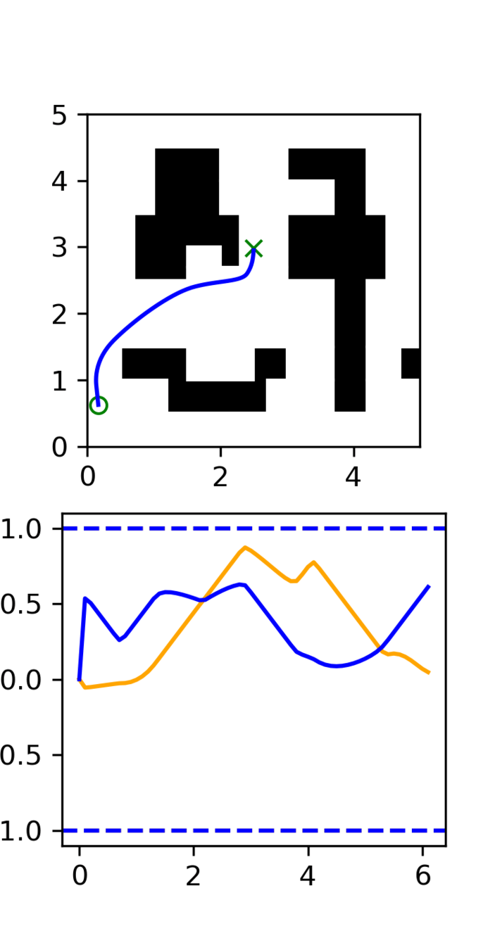
Results
\(|\mathcal{D}_S| = 50\), \(|\mathcal{D}_S| = 2000\), \(\epsilon\)-prediction with denoising loss
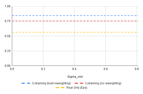
Results: Success Rate vs \(\sigma_{min}\)
Results: Success Rate vs \(\sigma_{min}\)
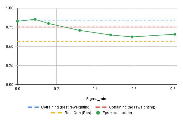
*
* \(\sigma_{min}=0\) and the red baseline should be approx. equal...
Results: Success Rate vs \(\sigma_{min}\)
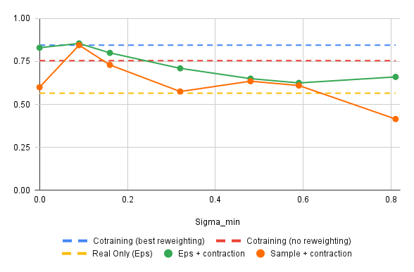
Results: Success Rate vs \(\sigma_{min}\)
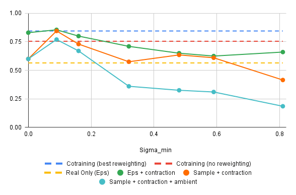
\(\sigma^*_{min}\) is small
Summary
- \(\epsilon\)-prediction > \(x_0\)-prediction
- "Best" policy used contraction (i.e. \(\sigma > \sigma_{min}\)), but no ambient loss
- Best \(\sigma_{min}\) was the low, but not zero
- In this set up... sim data is only slightly corrupt; high quality
- "Best" policy attains 85.5% success rate. Best baseline policy attains 84.5% success rate
- This is not statistically significant...
Discussion
This is an unfavorable setting for ambient diffusion
- Sim data is barely corrupt \(\implies\) effect of ambient diffusion is reduced
- Hyperparameters, sim, etc tuned for baseline
- Per-datapoint \(\sigma_{min}\)
- Scaling \(|\mathcal{D}_S|\) (cotraining plateau?)
- Cropping and locality ideas from ambient-o
- Tuned hyperparameters
Giannis and I think we can get the policy to over 90%..
Part 3
Next Directions
Next Directions
Hypothesis:
haven't test this yet... sorry Russ
- High-noise regime: planning, decision-making
- Low-noise regime: traj opt, control, interpolation, etc
Ambient-o provides a way to use corrupt data to learn in both of these regimes
- High-noise regime: contraction + ambient loss
- Low-noise regime: locality
Corruptions in Robotics
\(q_0\) Trajectory Quality
\(q_0\) Planning Quality
Experiment 1:
RRT vs GCS
Low
Medium
Corruption Regime
High-frequencies
Experiment 1: RRT vs GCS
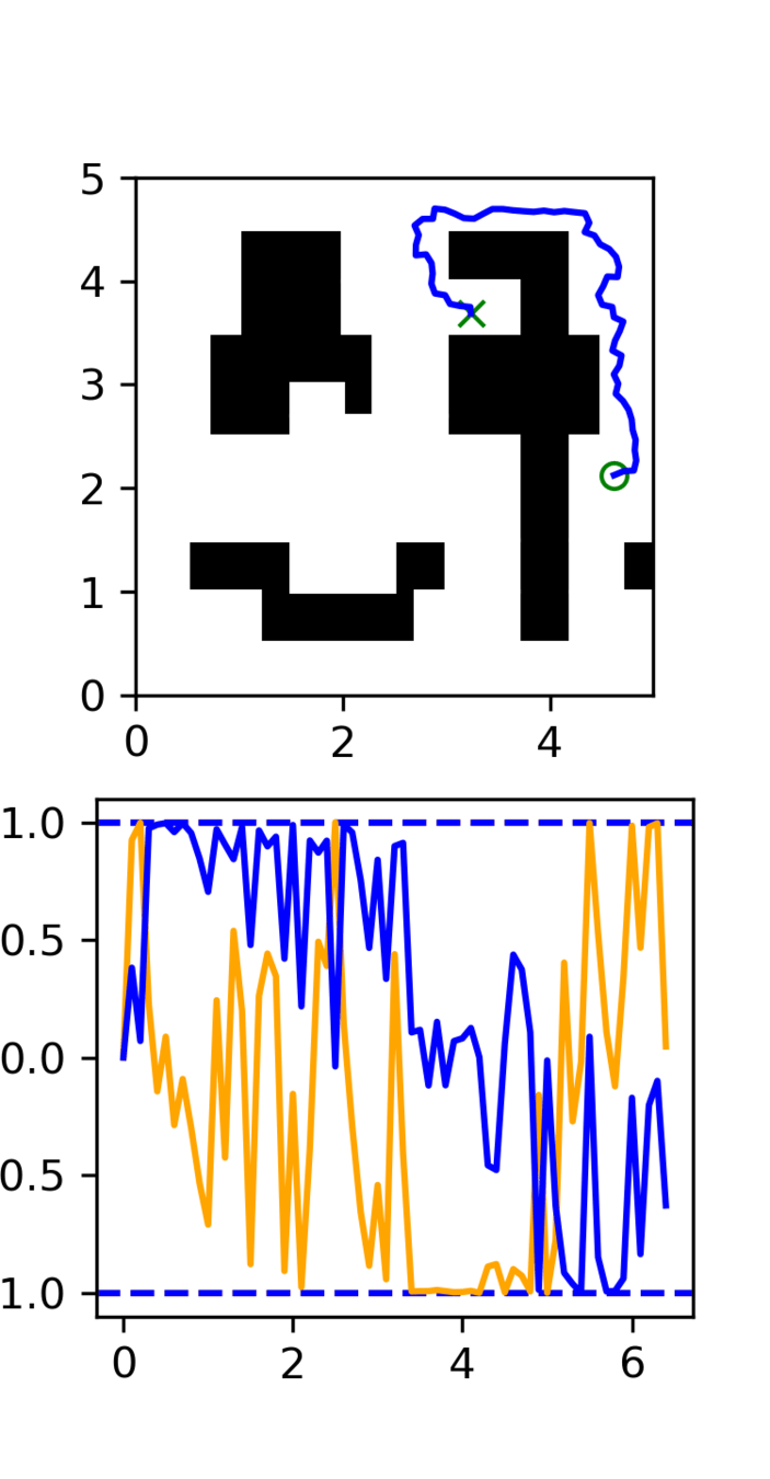
GCS
(clean)
RRT
(clean)
Task: Cotrain on GCS and RRT data
Goal: Sample clean and smooth GCS plans
- Example of high frequency corruption
- Common in robotics
- Low quality teleoperation or data gen
Corruptions in Robotics
\(q_0\) Trajectory Quality
\(q_0\) Planning Quality
Experiment 1:
RRT vs GCS
Low
Medium
Corruption Regime
High-frequencies
Experiment 2:
Cross-embodiment (Lu)
Low
Medium
Low-fequencies
Experiment 2: Lu's Data
- Same task + plan structure, different robot embodiment
- Plans are high quality
- Trajectories (EE-space) have embodiment gap (lower quality)
Corruptions in Robotics
\(q_0\) Trajectory Quality
\(q_0\) Planning Quality
Experiment 1:
RRT vs GCS
Experiment 3:
Bin Organization
Low
Medium
Medium
Incorrect
Corruption Regime
High-frequencies
Low-fequencies
Experiment 2:
Cross-embodiment (Lu)
Low
Medium
High-fequencies
Experiment 3
Task: Pick-and-place objects into specific bins
Clean Data: Demos with the correct logic
Corrupt Data: incorrect logic, Open-X, pick-and-place datasets, datasets with bins, etc
- Motions may be reasonable and informative
- But the decision making is incorrect
Locality
In image generation...
- At low noise-levels, denoising can be performed near-optimally using local patches
- Let crop(t) be the crop size required to diffuse optimally at time t
- Let \(A_p(t)\) and \(A_q(t)\) be random crops of images from p and q of size crop(t)
- If the distribution of \(A_p(t)\) and \(A_q(t)\) are similar, then images from q can be used to train a denoiser for p for noise levels < t
Locality
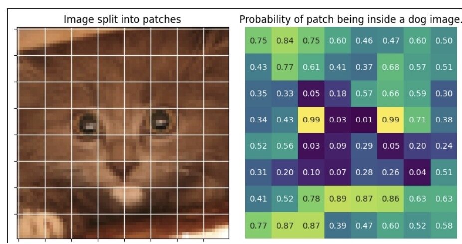
Cat images can be used to train a generative models for dogs!