Ambient Diffusion Update
Aug 14, 2025
Adam Wei
Agenda
- Book-keeping Items
- Effect of \(\sigma_{min}\)
- Effect of buffer
- Frequency Analysis
Book-keeping Items
- New version is finally on arXiv
- Will submit to a IROS and CoRL workshop
- 6DoF teleop is almost done!
Algorithm Overview
Repeat:
- Sample (O, A, \(\sigma_{min}\)) ~ \(\mathcal{D}\)
- Choose noise level \(\sigma > \sigma_{min}\)
- Optimize denoiser or ambient loss
\(\sigma=1\)
\(\sigma=0\)
\(\sigma=\sigma_{min}\)
Corrupt Data (\(\sigma_{min}\geq0\))
Clean Data (\(\sigma_{min}=0\))
Loss Function (for \(x_0\sim q_0\))
\(\mathbb E[\lVert h_\theta(x_t, t) + \frac{\sigma_{min}^2\sqrt{1-\sigma_{t}^2}}{\sigma_t^2-\sigma_{min}^2}x_{t} - \frac{\sigma_{t}^2\sqrt{1-\sigma_{min}^2}}{\sigma_t^2-\sigma_{min}^2} x_{t_{min}} \rVert_2^2]\)
Ambient Loss
Denoising Loss
\(x_0\)-prediction
\(\epsilon\)-prediction
(assumes access to \(x_0\))
(assumes access to \(x_{t_{min}}\))
\(\mathbb E[\lVert h_\theta(x_t, t) - x_0 \rVert_2^2]\)
\(\mathbb E[\lVert h_\theta(x_t, t) - \epsilon \rVert_2^2]\)
\(\mathbb E[\lVert h_\theta(x_t, t) - \frac{\sigma_t^2 (1-\sigma_{min}^2)}{(\sigma_t^2 - \sigma_{min}^2)\sqrt{1-\sigma_t^2}}x_t + \frac{\sigma_t \sqrt{1-\sigma_t^2}\sqrt{1-\sigma_{min}^2}}{\sigma_t^2 - \sigma_{min}^2}x_{t_{min}}\rVert_2^2]\)
How to choose \(\sigma_{min}\)
Granularity
- Per dataset
- Per datapoint
Choosing \(\sigma_{min}\)
- Sweep \(\sigma_{min} \in [0,1]\)
- Train a classifier
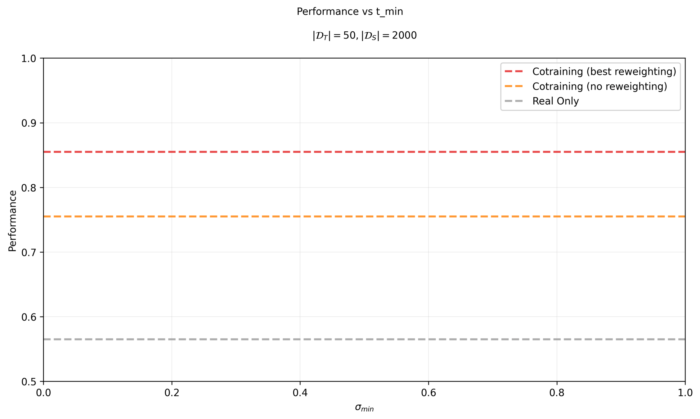
Previous results: per dataset and sweep \(\sigma_{min}\)
"Clean" Data
"Corrupt" Data
\(|\mathcal{D}_T|=50\)
\(|\mathcal{D}_S|=2000\)
Eval criteria: Success rate for planar pushing across 200 randomized trials
Datasets and Task
Sweep \(\sigma_{min}\) per dataset
Previous results: per dataset and sweep \(\sigma_{min}\)
Sweep \(\sigma_{min}\) per dataset
Previous results: per dataset and sweep \(\sigma_{min}\)
Choosing \(\sigma_{min}\): Classifier
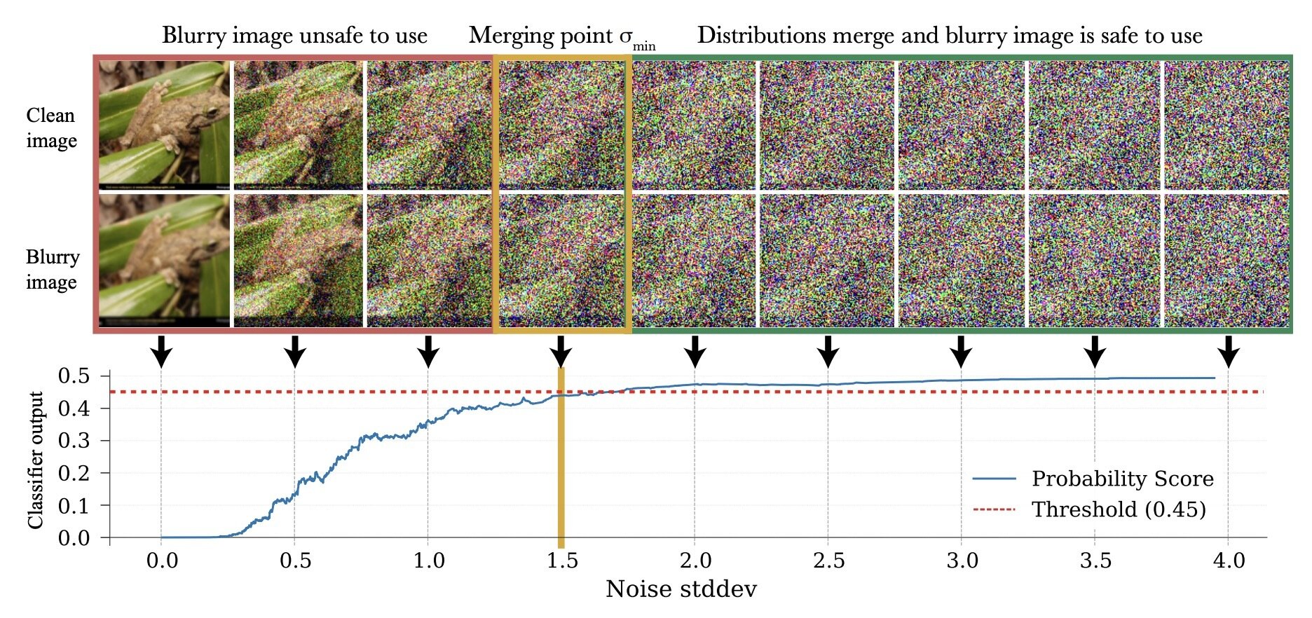
\(\sigma_{min}^i = \inf\{\sigma\in[0,1]: c_\theta (x_\sigma, \sigma) > 0.5-\epsilon\}\)
\(p_0\)
\(q_0\)
\(\implies \sigma_{min}^i = \inf\{\sigma\in[0,1]: d_\mathrm{TV}(p_\sigma, q_\sigma) < \epsilon\}\)*
* assuming \(c_\theta\) is perfectly trained
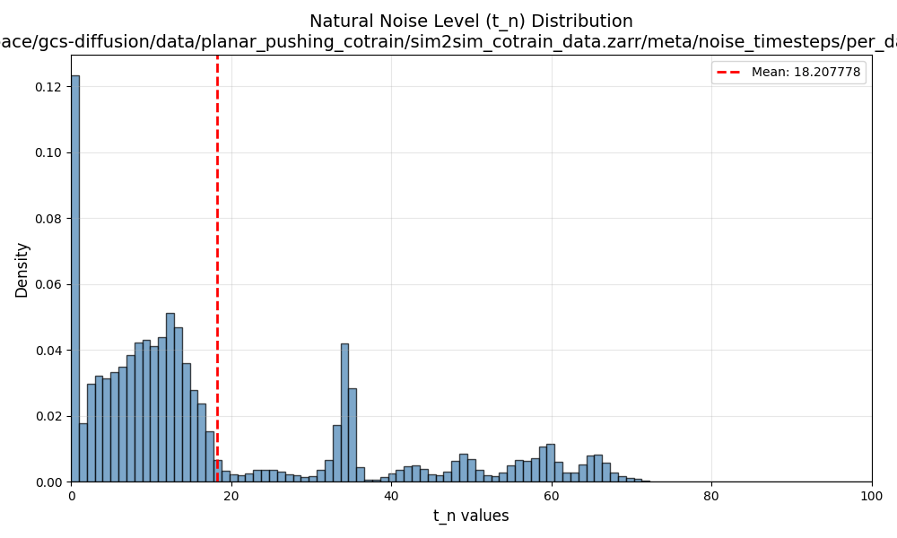
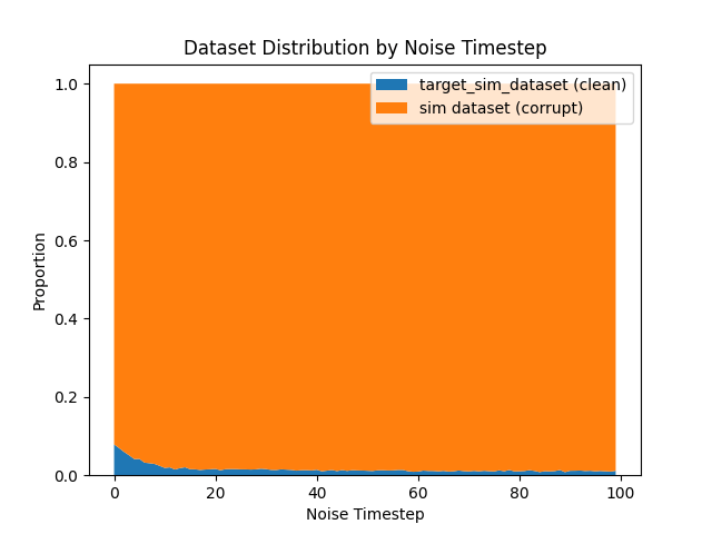
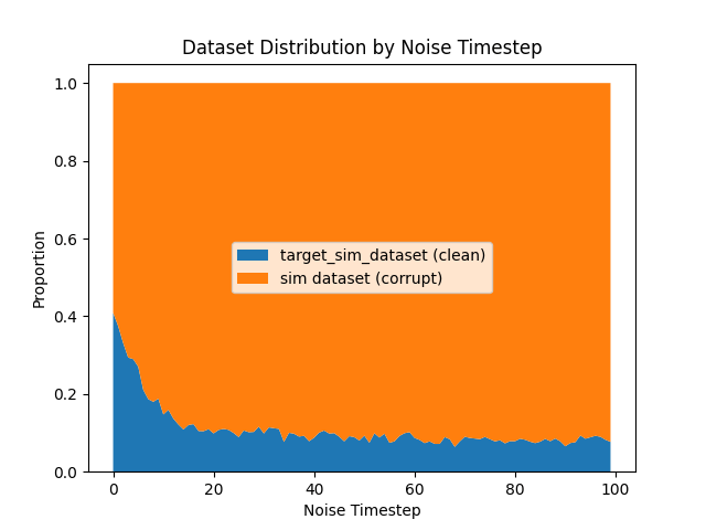
Distribution of \(\sigma_{min}\) in \(\mathcal{D}_S\)
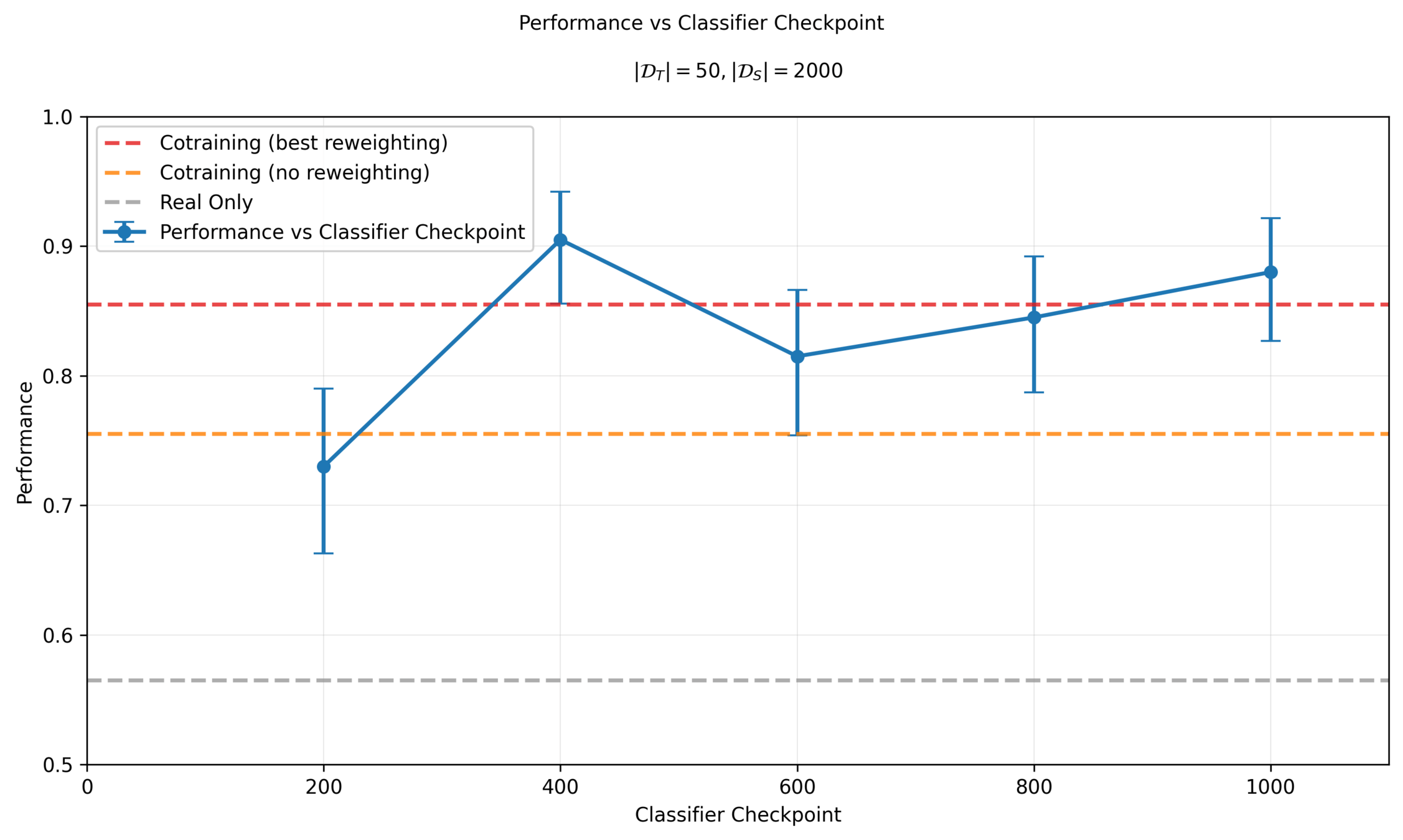
Results: Classifier \(\sigma_{min}\)
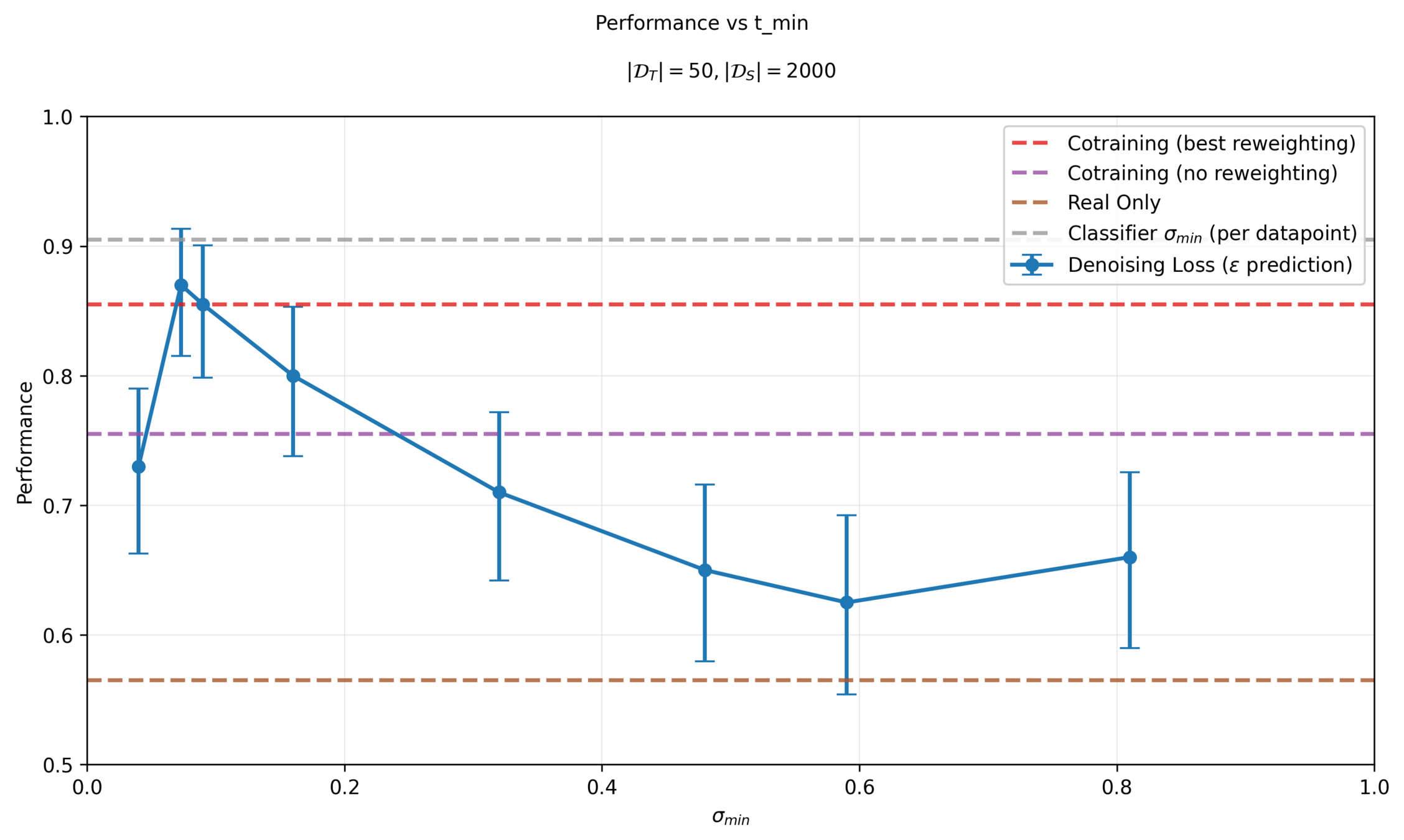
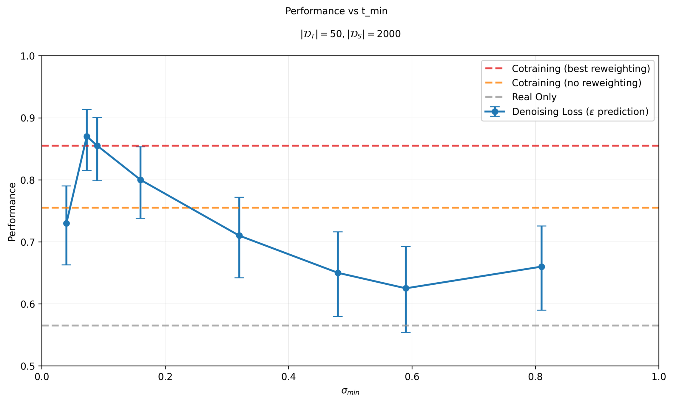
Sensitivity to \(\sigma_{min}\)
Different checkpoints will choose different \(\sigma_{min}\)
Epoch 400: average \(t_{min}^i\) is 18.2
Epoch 800: average \(t_{min}^i\) is 19.99
Stronger checkpoints\(\implies\) larger \(\sigma_{min}\) required to fool classifier \(\implies\) use corrupt data less
Sensitivity to \(\sigma_{min}\)
Performance is sensitive to classifier and \(\sigma_{min}\) choice!
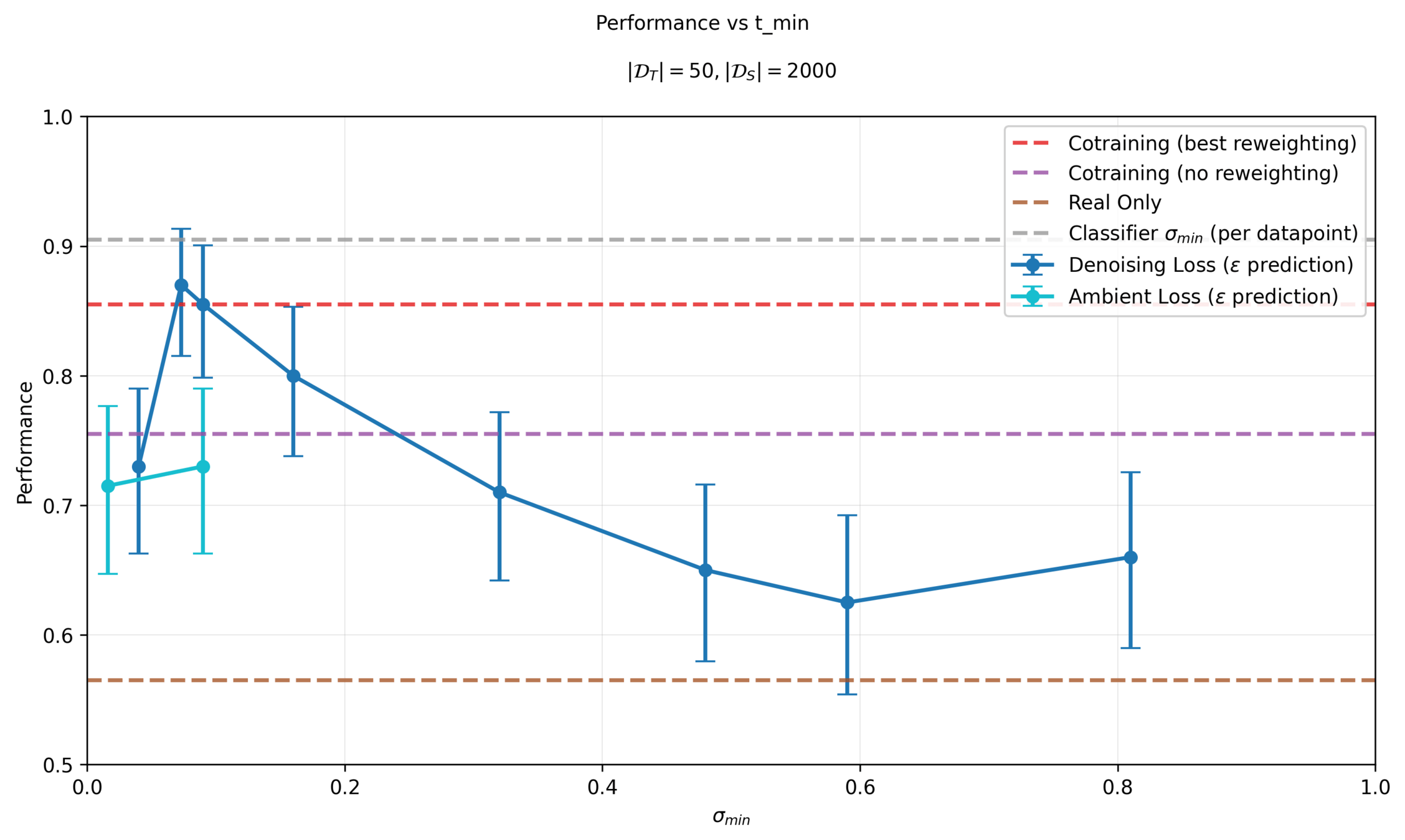
Denoising Loss vs Ambient Loss
Denoising Loss vs Ambient Loss
Denoising Loss vs Ambient Loss
\(\sigma=1\)
\(\sigma=0\)
\(\mathbb E[\lVert h_\theta(x_t, t) - x_0 \rVert_2^2]\)
Corrupt Data: ambient loss
\( x_0 \sim p_0\)
\( y_0 \sim q_0\)
\(\sigma=\sigma_{min}\)
\(\mathbb E[\lVert h_\theta(y_t, t) + \frac{\sigma_{min}^2\sqrt{1-\sigma_{t}^2}}{\sigma_t^2-\sigma_{min}^2}y_{t} - \frac{\sigma_{t}^2\sqrt{1-\sigma_{min}^2}}{\sigma_t^2-\sigma_{min}^2} y_{t_{min}} \rVert_2^2]\)
Clean Data: denoising loss
Key insight: if \(\sigma \approx \sigma_{min}\), ambient loss has division by 0 !
Denoising Loss vs Ambient Loss
Denoising Loss vs Ambient Loss
\(\sigma=1\)
\(\sigma=0\)
\(\mathbb E[\lVert h_\theta(x_t, t) - x_0 \rVert_2^2]\)
\( x_0 \sim p_0\)
\( y_0 \sim q_0\)
\(\sigma=\sigma_{min}\)
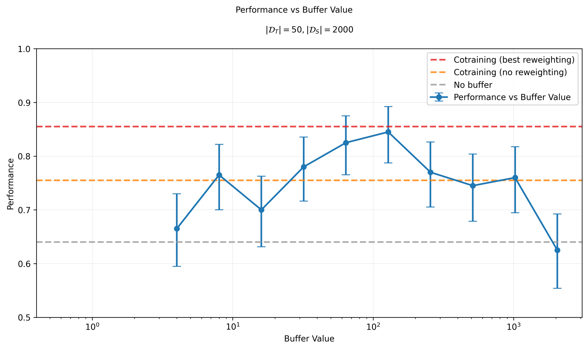
\(\sigma_{buffer}(\sigma_{min}, \sigma_t)\)
\(\mathbb E[\lVert h_\theta(y_t, t) + \frac{\sigma_{min}^2\sqrt{1-\sigma_{t}^2}}{\sigma_t^2-\sigma_{min}^2}y_{t} - \frac{\sigma_{t}^2\sqrt{1-\sigma_{min}^2}}{\sigma_t^2-\sigma_{min}^2} y_{t_{min}} \rVert_2^2]\)
Clean Data: denoising loss
Key insight: Add buffer to stabilize training (avoid division by 0)
Corrupt Data: ambient loss
Denoising Loss vs Ambient Loss
Ambient Diffusion: Effect of Buffer
Denoising Loss vs Ambient Loss
Ambient Diffusion: Scaling \(|\mathcal{D}_S|\)

* denoising loss
Denoising Loss vs Ambient Loss
Ambient Diffusion: Scaling \(|\mathcal{D}_S|\)
Hypothesis: Ambient loss underperforms denoising loss for small \(\mathcal{D}_S\) but may scale better
\(|\mathcal{D}_S|=500\)
\(|\mathcal{D}_S|=8000\)
Denoising Loss vs Ambient Loss
Ambient Diffusion: Scaling \(|\mathcal{D}_S|\)
Hypothesis: Ambient loss underperforms denoising loss for small \(\mathcal{D}_S\) but may scale better
\(\mathbb E[\lVert h_\theta(x_t, t) + \frac{\sigma_{min}^2\sqrt{1-\sigma_{t}^2}}{\sigma_t^2-\sigma_{min}^2}x_{t} - \frac{\sigma_{t}^2\sqrt{1-\sigma_{min}^2}}{\sigma_t^2-\sigma_{min}^2} x_{t_{min}} \rVert_2^2]\)
Ambient Loss
Denoising Loss
\(x_0\)-prediction
(assumes access to \(x_0\))
(assumes access to \(x_{t_{min}}\))
\(\mathbb E[\lVert h_\theta(x_t, t) - x_0 \rVert_2^2]\)
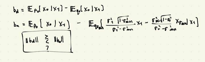
- Bias since \(x_0\sim q_0\) and \(p_0\neq q_0\)
- Larger \(\mathcal{D}_S \implies\) more samples with bias
- lower bias since \(x_{\sigma_{min}}\sim q_{\sigma_{min}} \) and \(p_{\sigma_{min}} \approx q_{\sigma_{min}}\)
- Worse sample complexity due to noisy MSE targets
- But (potentially) better scaling due to reduced bias

Denoising Loss vs Ambient Loss
Ambient Diffusion: Bias?
Hypothesis: Ambient loss underperforms denoising loss for small \(\mathcal{D}_S\) but may scale better
Denoising Loss vs Ambient Loss
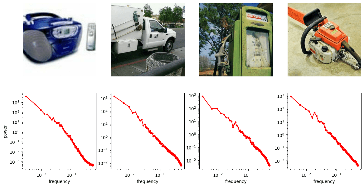
Frequency Analysis: Computer Vision
Denoising Loss vs Ambient Loss
Frequency Analysis: Computer Vision
Denoising Loss vs Ambient Loss
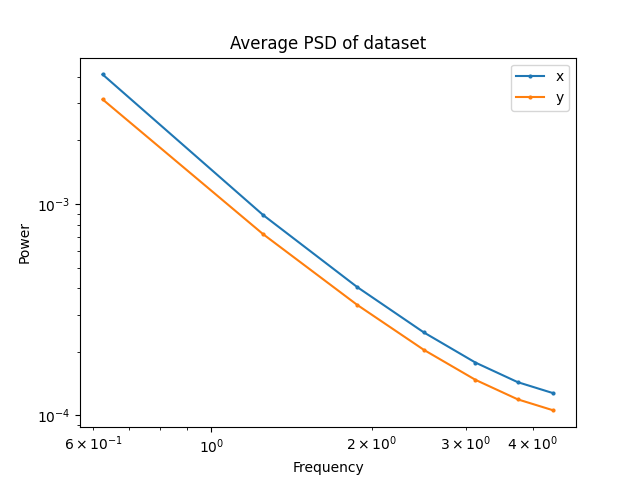
Frequency Analysis: Robotics
Questions:
- Does robotics data follow a similar power law in frequency domain?
- What does the corruption look like in the frequency domain*
* Ambient diffusion is most effective for high-frequency corruptions
Denoising Loss vs Ambient Loss
Frequency Analysis: Robotics
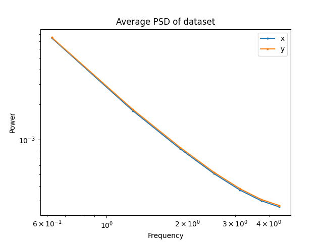
Maze: RRT
Maze: GCS
T-Pushing: GCS
T-Pushing: Human
Denoising Loss vs Ambient Loss
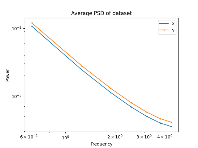
Frequency Analysis: Robotics
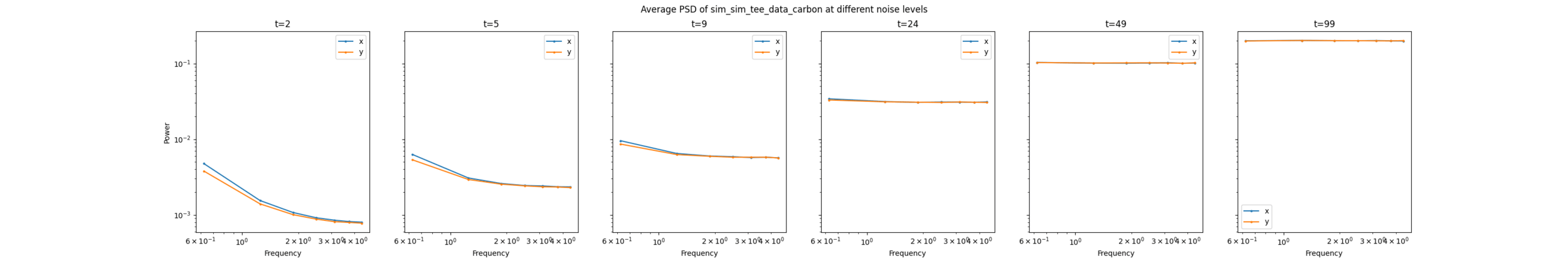
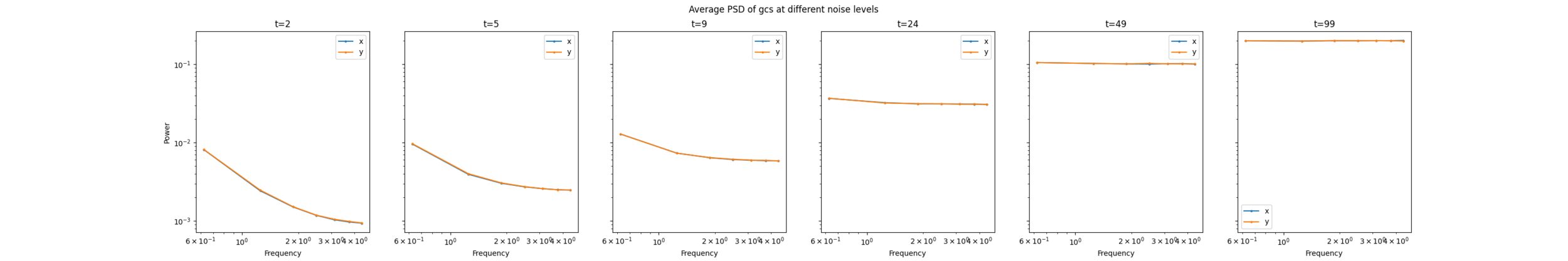
T-Pushing: Human
Maze: GCS
Denoising Loss vs Ambient Loss
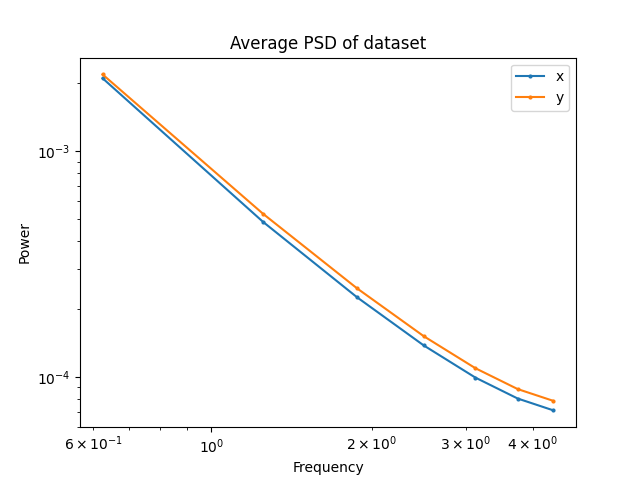
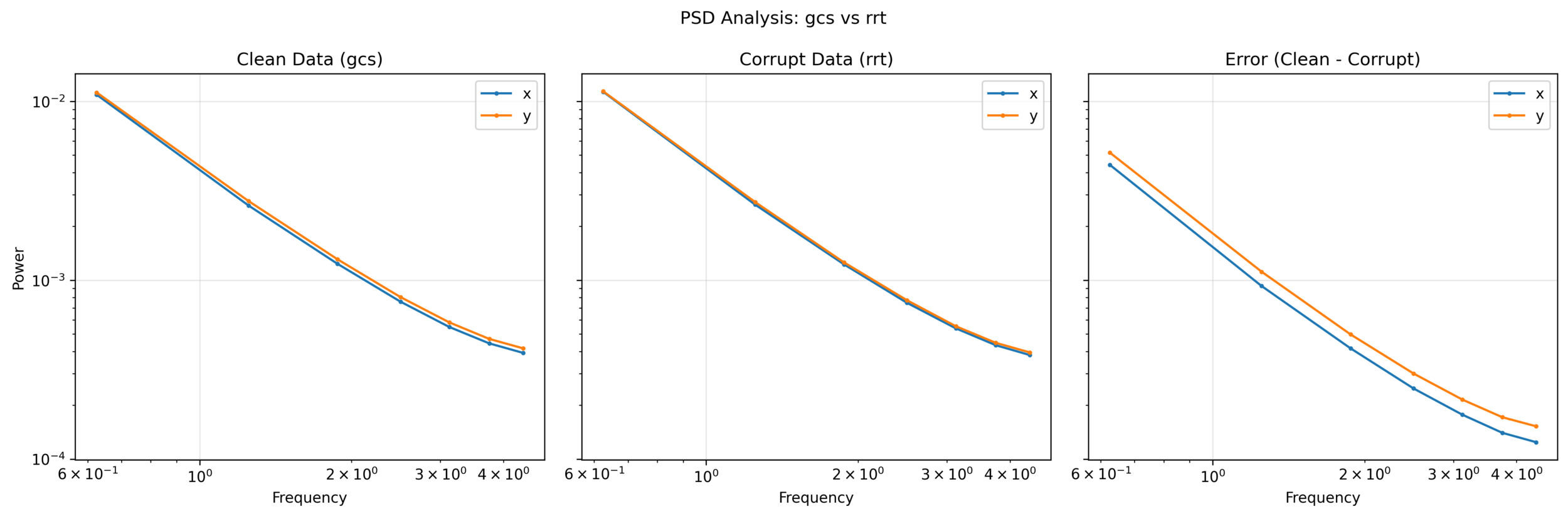
Frequency Analysis: Corruption
Goal: Characterize the nature of the corruption
- Higher-noise corruption is better, but not needed
For every clean sequence:
- Identify the nearest state neighbors in the corrupt data
- Compute PSD of the difference in actions
Average the PSDs of the ~10,000 closest state neighbors
Denoising Loss vs Ambient Loss
Frequency Analysis: Corruption
Denoising Loss vs Ambient Loss
Frequency Analysis: Corruption

Denoising Loss vs Ambient Loss
Next Directions
Giannis and I are thinking of some other exciting ideas in this direction...
... more on this once results are available! :D