Amazon CoRo June Update
Jun 19, 2025
Adam Wei
Agenda
- Algorithm Overview + Implementations
- Sim + Real Experiments
- GCS + RRT Experiments
- Next Directions
Part 1
Ambient Diffusion Recap
and Implementations
Ambient Diffusion
Learning from "clean" (\(p_0\)) and "corrupt" data (\(q_0\))
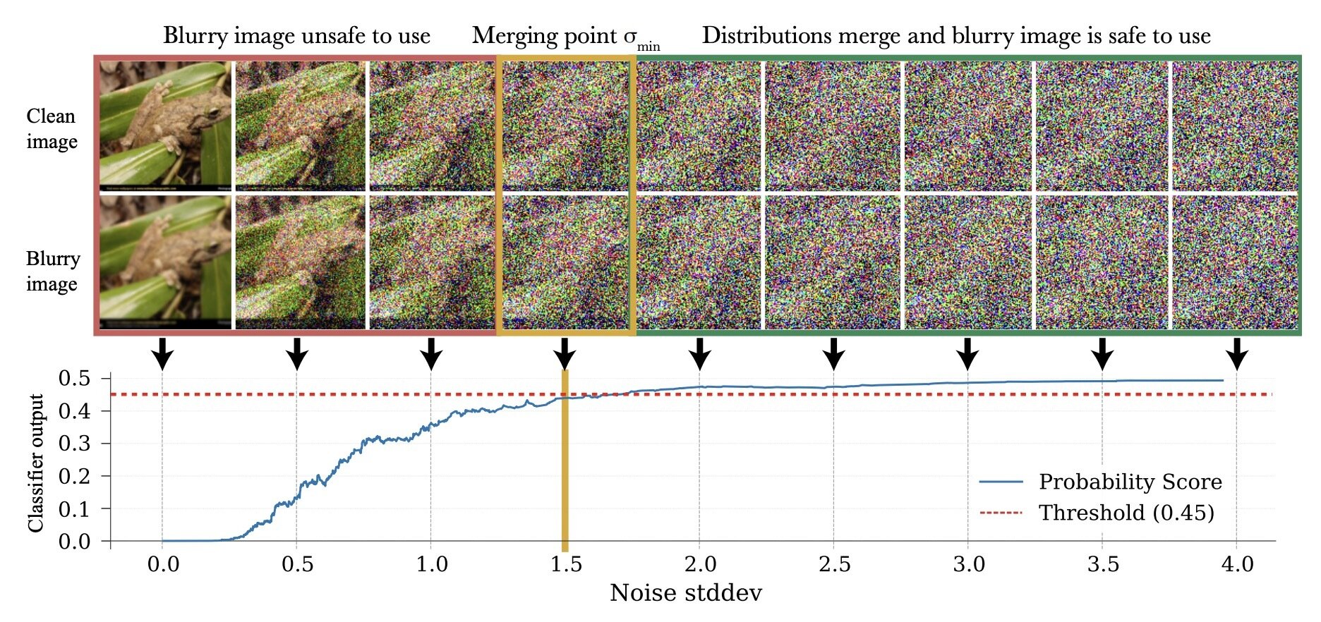
Learning in the high-noise regime
\(\exists \sigma_{min}\) s.t. \(d_\mathrm{TV}(p_{\sigma_{min}}, q_{\sigma_{min}}) < \epsilon\)
- Only use samples from \(q_0\) to train denoisers with \(\sigma > \sigma_{min}\)
- Corruption level of each datapoint determines its utility
\(\sigma=1\)
\(\sigma=0\)
\(\sigma=\sigma_{min}\)
Clean Data
Corrupt Data
Learning in the high-noise regime
\(\exists \sigma_{min}\) s.t. \(d_\mathrm{TV}(p_{\sigma_{min}}, q_{\sigma_{min}}) < \epsilon\)
(in this example, \(\epsilon = 0.05\))
\(p_0\)
\(q_0\)
Learning in the high-noise regime
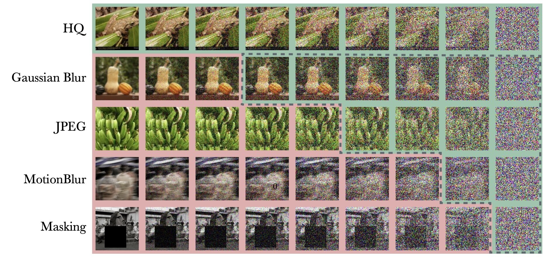
Factors that affect \(\sigma_{min}\):
- Similarity of \(p_0\), \(q_0\)
- Nature of the corruption from \(p_0\) to \(q_0\)
- Contracting \(q_{\sigma_{min}}\) towards \(p_{\sigma_{min}}\) "masks" corruption between \(p_0\) and \(q_0\)
... but also destroys useful signal
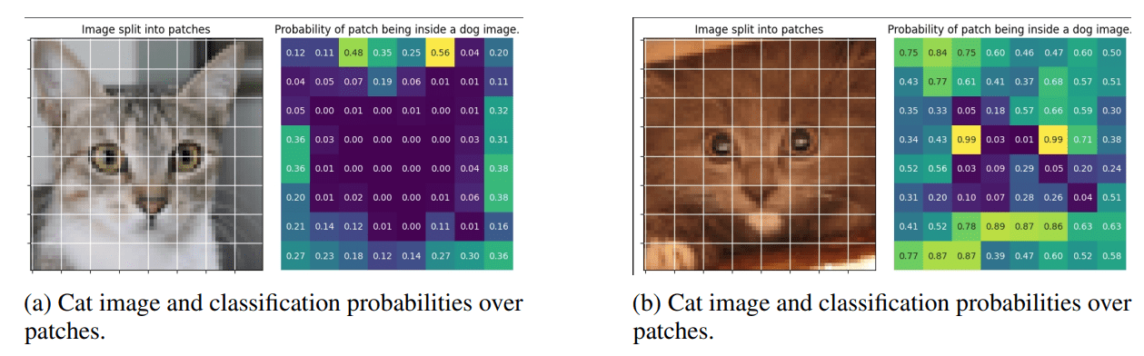
Contraction as masking
- Contracting \(q_{\sigma_{min}}\) towards \(p_{\sigma_{min}}\) "masks" corruption between \(p_0\) and \(q_0\)
... but also destroys useful signal
More info lost
Learning in the high-noise regime
\(\exists \sigma_{min}\) s.t. \(d_\mathrm{TV}(p_{\sigma_{min}}, q_{\sigma_{min}}) < \epsilon\)
- Only use samples from \(q_0\) to train denoisers with \(\sigma > \sigma_{min}\)
- Corruption level of each datapoint determines its utility
\(\sigma=1\)
\(\sigma=0\)
\(\sigma=\sigma_{min}\)
Denoising Loss
Denoising OR Ambient Loss
Loss Function (for \(x_0\sim q_0\))
\(\mathbb E[\lVert h_\theta(x_t, t) + \frac{\sigma_{min}^2\sqrt{1-\sigma_{t}^2}}{\sigma_t^2-\sigma_{min}^2}x_{t} - \frac{\sigma_{t}^2\sqrt{1-\sigma_{min}^2}}{\sigma_t^2-\sigma_{min}^2} x_{t_{min}} \rVert_2^2]\)
Ambient Loss
Denoising Loss
\(x_0\)-prediction
\(\epsilon\)-prediction
(assumes access to \(x_0\))
(assumes access to \(x_{t_{min}}\))
\(\mathbb E[\lVert h_\theta(x_t, t) - x_0 \rVert_2^2]\)
\(\mathbb E[\lVert h_\theta(x_t, t) - \epsilon \rVert_2^2]\)
\(\mathbb E[\lVert h_\theta(x_t, t) - \frac{\sigma_t^2 (1-\sigma_{min}^2)}{(\sigma_t^2 - \sigma_{min}^2)\sqrt{1-\sigma_t^2}}x_t + \frac{\sigma_t \sqrt{1-\sigma_t^2}\sqrt{1-\sigma_{min}^2}}{\sigma_t^2 - \sigma_{min}^2}x_{t_{min}}\rVert_2^2]\)
Sanity check: ambient loss \(\rightarrow\) denoising loss as \(\sigma_{min} \rightarrow 0\)
Experiments: Test all 4
Implementation Details
- Sample noise level first, then data points
- Ambient loss "buffer" for training stability
- Contract each datapoint once
- Other small details...
Implementation details: included for completeness...
Learning in the low-noise regime
Can use OOD data to learn in the low-noise regime...
... more on this next time
Part 2
Sim + Real Experiments
"Clean" Data
"Corrupt" Data
\(|\mathcal{D}_T|=50\)
\(|\mathcal{D}_S|=2000\)
Eval criteria: Success rate for planar pushing across 200 randomized trials
Datasets and Task
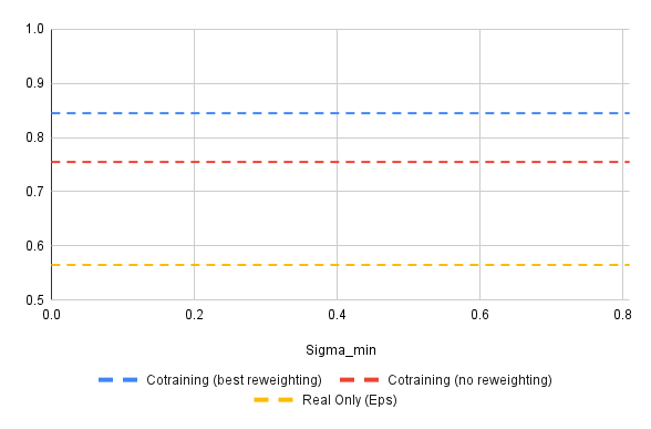
Results
Experiments
Choosing \(\sigma_{min}\): Swept several values on the dataset level
Loss function: Tried all 4 combinations of
{\(x_0\)-prediction, \(\epsilon\)-prediction} x {denoising, ambient}
Preliminary Observations
(will present best results on next slide)
- \(\epsilon\)-prediction > \(x_0\)-prediction and denosing > ambient loss
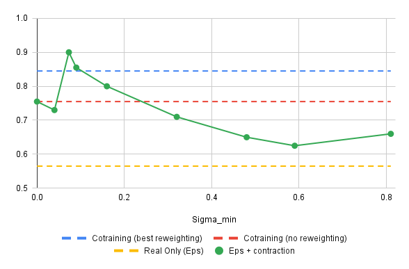
- Small (but non-zero) \(\sigma_{min}\) performed best
- Ambient diffusion scales slightly better with more sim data than cotraining
Results
\(|\mathcal{D}_S| = 50\), \(|\mathcal{D}_S| = 2000\), \(\epsilon\)-prediction with denoising loss
Results
\(|\mathcal{D}_S| = 50\), \(|\mathcal{D}_S| = 2000\), \(\epsilon\)-prediction with denoising loss
Part 3
Maze Experiments
Experiment: RRT vs GCS
GCS
(clean)
RRT
(clean)
Task: Cotrain on GCS and RRT data
Goal: Sample clean and smooth GCS plans
- Example of high frequency corruption
- Common in robotics
- Low quality teleoperation or data gen
Baselines
Success Rate: 50%
Average Jerk Squared: 7.5k
100 GCS Demos
Success Rate: 99%
Average Jerk Squared: 2.5k
4950 GCS Demos
Success Rate: 100%
Average Jerk Squared: 17k
4950 RRT Demos
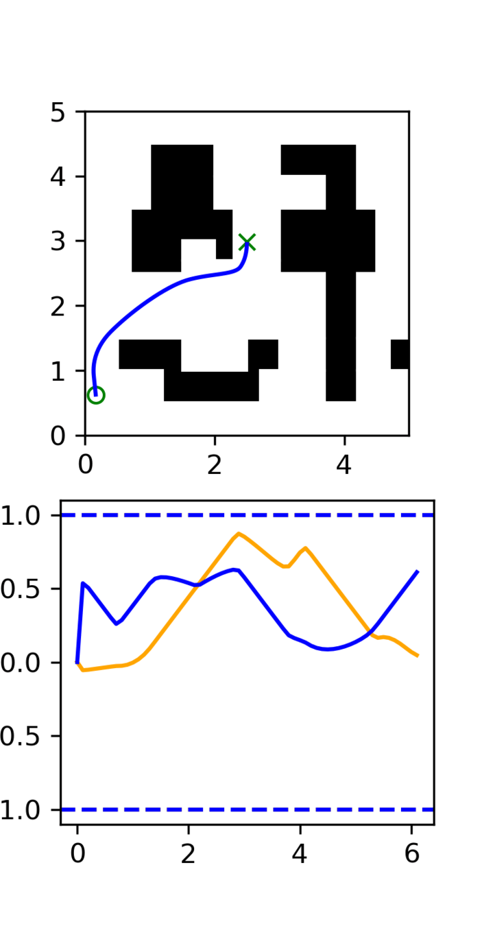
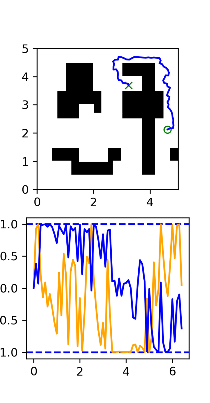
Cotraining vs Ambient Diffusion
Success Rate: 91%
Average Jerk Squared: 12.5k
Cotraining: 100 GCS Demos, 5000 RRT Demos, \(x_0\)-prediction
Success Rate: 98%
Average Jerk Squared: 5.5k
Ambient: 100 GCS Demos, 5000 RRT Demos, \(x_0\)-prediction ambient loss
See plots for qualitative results
Part 4
Next Experiments
North Star Goal
Main goal: Cotrain with ambient diffusion using internet data (Open-X, AgiBot, etc) and/or simulation data
... but first some "stepping stone" experiments
Stepping stone experiments are designed to
- Sanity check and debug implementations along the way
- Highlight and isolate specific components of the algorithm
- Improve exposition in the final paper
Experiment: Extend Maze to MP
Corrupt data: RRT/low quality data from 20-30 different environments
Clean data: GCS data from 2-3 environments
Performance metric: Success rate + smoothness metrics in seen/unseen environments
Purpose: Test learning in the high-noise regime
Experiment: Lu's Data
- Same task + plan structure, different robot embodiment
- Plans are high quality
- Trajectories (EE-space) have embodiment gap (lower quality)
Purpose: Test learning in the high-noise regime
Experiment: Bin Sorting
Task: Pick-and-place objects into specific bins
Clean Data: Demos with the correct logic
Corrupt Data: incorrect logic, Open-X, pick-and-place datasets, datasets with bins, etc
- Motions may be reasonable and informative
- But the decision making is incorrect
Purpose: Test learning in the low-noise regime
Experiment Document
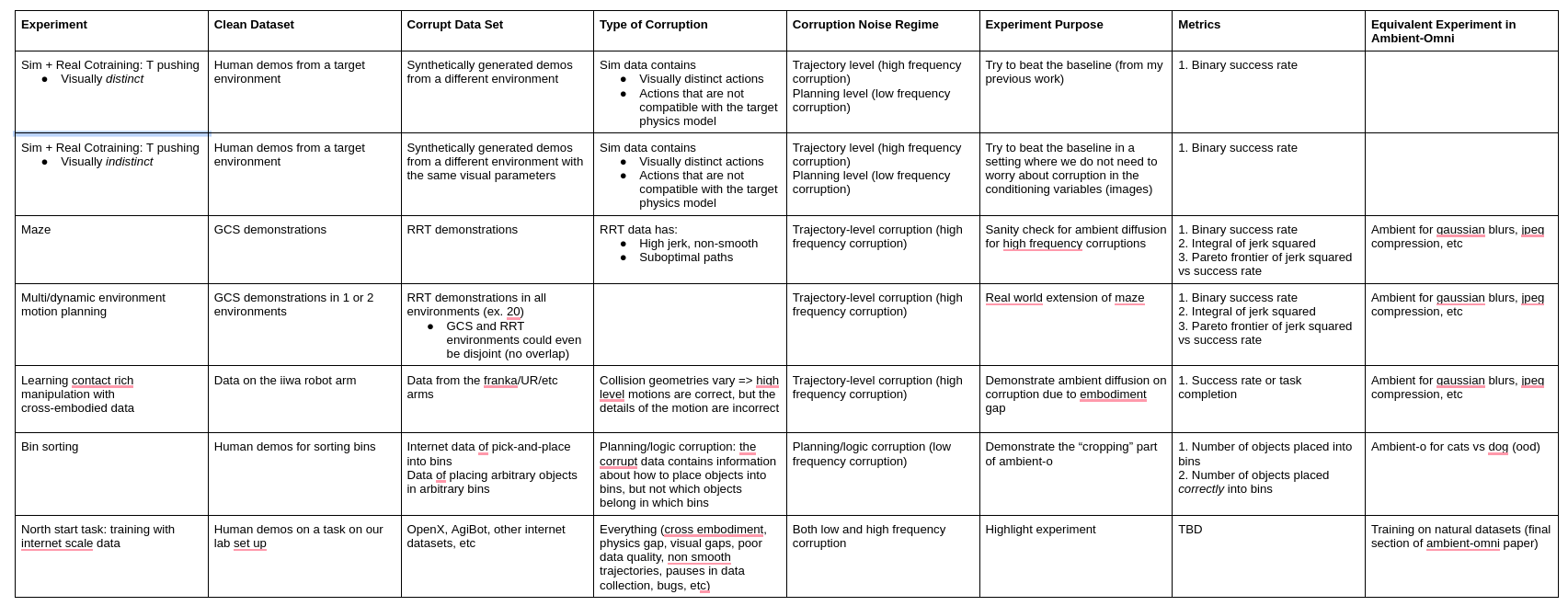
Details outlined in a google doc. Can share link privately if interested