June 8, 2026

Adam Wei

Ambient Diffusion Policy

Imitation Learning From Suboptimal Data in Robotics

Agenda

Problem Statement
Ambient Diffusion Policy
Why does this work?
Results
Limitations + Future Directions

Key takeaways!

Results are good...

Part 1

Problem Statement

"Suboptimal" Data Is Abundant

Sim2real gaps
Noisy or non-expert teleop
Task-level mismatch
Changes in low-level controller

Embodiment gap
Camera models, poses, etc
Different environment, objects, etc

Open-X

In-Distribution Data

simulation

Suboptimal / OOD Data

Utility of Suboptimal Data

But there is still value and utility in OOD data!

... we just aren't using it correctlty

Open-X

In-Distribution Data

simulation

Suboptimal / OOD Data

Problem Statement

Open-X

In-Distribution Data

simulation

Suboptimal / OOD Data

Colab w/ Giannis Daras

What are principled algorithms for learning from suboptimal data sources?

\(p\)

\(q\)

"Suboptimal" Data Is Abundant

Q. What does "suboptimal" actions mean?

A. You decide 😊

Low-quality
High-quality, but out-of-distribution
Hand tracking data, UMI, etc

Open-X

In-Distribution Data

simulation

Suboptimal / OOD Data

Part 2

Ambient Diffusion Policy

Diffusion Training

\(t=0\)

\(t=T\)

"High-quality" Data

For all \(t \in [0,T]\): train \(h_\theta(A_t, O, t) \approx \mathbb{E}[A_0 \mid A_t, O]\)

Co-training

For all \(t \in [0,T]\): train \(h_\theta(A_t, O, t) \approx \mathbb{E}[A_0 \mid A_t, O]\)

"Suboptimal" Data

"High-quality" Data

\(t=0\)

\(t=T\)

Co-training

For all \(t \in [0,T]\): train \(h_\theta(A_t, O, t) \approx \mathbb{E}[A_0 \mid A_t, O]\)

"Suboptimal" Data

"High-quality" Data

\(t=0\)

\(t=T\)

\(\alpha\)

\(1-\alpha\)

\(p^{train} = \alpha\) \(p\)\(+(1-\alpha)\) \(q\)

\(p^{train}\) contains \(q\) \(\implies\) This is the wrong objective

\(\pi(A|O)\) learns both the good and the bad features of \(q\)

Ambient Diffusion Policy

\(t_{\min}\)

\(t> t_{\min}\)

"High-quality" Data

\(p_t\) \(\not\approx\) \(q_t\)

\(p_t\) \(\approx\) \(q_t\)

\(t=T\)

For all \(t \in [0,T]\): train \(h_\theta(A_t, O, t) \approx \mathbb{E}[A_0 \mid A_t, O]\)

\(t=0\)

Gaussian Noise As Contraction

\(p_0\)

\(q_0\)

\(p_t\)

\(q_t\)

D(p_0, q_0) \geq D(p_t, q_t)

\(D(p_t, q_t) \to 0\) as \(t\to \infty\)

\(\implies \exists t_{min} \ \mathrm{s.t.}\ D(p_t, q_t) < \epsilon\ \forall t \in (t_{min}, T]\)

Noisy Channel

\(Y = X + \sigma_t Z\)

\(D(p_0, q_0)\)

\(D(p_t, q_t)\)

Ambient Diffusion Policy

\(t_{\min}\)

\(t> t_{\min}\)

"High-quality" Data

\(p_t\) \(\not\approx\) \(q_t\)

\(p_t\) \(\approx\) \(q_t\)

\(t=T\)

For all \(t \in [0,T]\): train \(h_\theta(A_t, O, t) \approx \mathbb{E}[A_0 \mid A_t, O]\)

\(t=0\)

Loss Function

Loss Function (for \(x_0\sim q_0\))

Denoising Loss vs Ambient Loss

Choosing \(\sigma_{min}\)

How to choose \(t_{min}\)?

\(\sigma_{t_{min}}\)

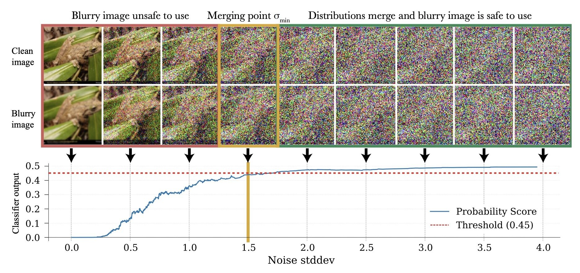
At high noise, high quality and low-quality actions are indistinguishable

Suff: if a classifier cannot reliable discern \(p_t\) and \(q_t\), then the data is safe to use

Loss Function

Loss Function (for \(x_0\sim q_0\))

Denoising Loss vs Ambient Loss

How to choose \(t_{min}\)?

Increasing granularity

Assign \(t_{min}\) per datapoint

Assign \(t_{min}\) per dataset

Run the classifier per dataset

Run the classifier per datapoint

We will see examples across this spectrum...

Ambient Diffusion Policy

\(t_{\min}\)

\(t> t_{\min}\)

"High-quality" Data

\(p_t\) \(\approx\) \(q_t\)

\(t=T\)

For all \(t \in [0,T]\): train \(h_\theta(A_t, O, t) \approx \mathbb{E}[A_0 \mid A_t, O]\)

\(t<t_{\max}\)

"Locality"

Both intervals \([0, t_{max})\) and \((t_{min}, T]\) have interpretations. More on this later...

\(t=0\)

\(t_{\max}\)

Implementation: Very simple!!

\(t_{\min}\)

\(t> t_{\min}\)

"High-quality" Data

\(t=T\)

For all \(t \in [0,T]\): train \(h_\theta(A_t, O, t) \approx \mathbb{E}[A_0 \mid A_t, O]\)

\(t<t_{\max}\)

Sample diffusion time, \(t\)
Sample admissible datapoint from \(\mathcal{D}_p \cup \mathcal{D}_q\)

\(t_{\max}\)

\(t=0\)

Implementation: Very simple!!

\(t_{\min}\)

\(t> t_{\min}\)

"High-quality" Data

\(t=T\)

\(t<t_{\max}\)

Sample diffusion time, \(t\)
Sample admissible datapoint from \(\mathcal{D}_p \cup \mathcal{D}_q\)

\(t_{\max}\)

\(t=0\)

Question break!

Part 3

Why Does This Work?

Answer

The structure of robot data

Ambient Diffusion Policy

\(t_{\min}\)

\(t> t_{\min}\)

"High-quality" Data

\(t=T\)

For all \(t \in [0,T]\): train \(h_\theta(A_t, O, t) \approx \mathbb{E}[A_0 \mid A_t, O]\)

\(t<t_{\max}\)

\(t_{\max}\)

\(p_t\) \(\approx\) \(q_t\)

"Locality"

Both intervals \([0, t_{max})\) and \((t_{min}, T]\) have interpretations.

\(t=0\)

Ambient Diffusion Policy

\(t_{\min}\)

\(t> t_{\min}\)

"High-quality" Data

\(t=T\)

For all \(t \in [0,T]\): train \(h_\theta(A_t, O, t) \approx \mathbb{E}[A_0 \mid A_t, O]\)

\(t_{\max}\)

\(p_t\) \(\approx\) \(q_t\)

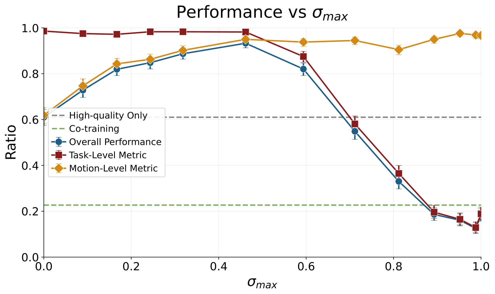
Utility of \(q\) is highest when \(t_{min}\) is small.

\(t=0\)

Let's start with \((t_{min}, T]\).

Loss Function

Loss Function (for \(x_0\sim q_0\))

Denoising Loss vs Ambient Loss

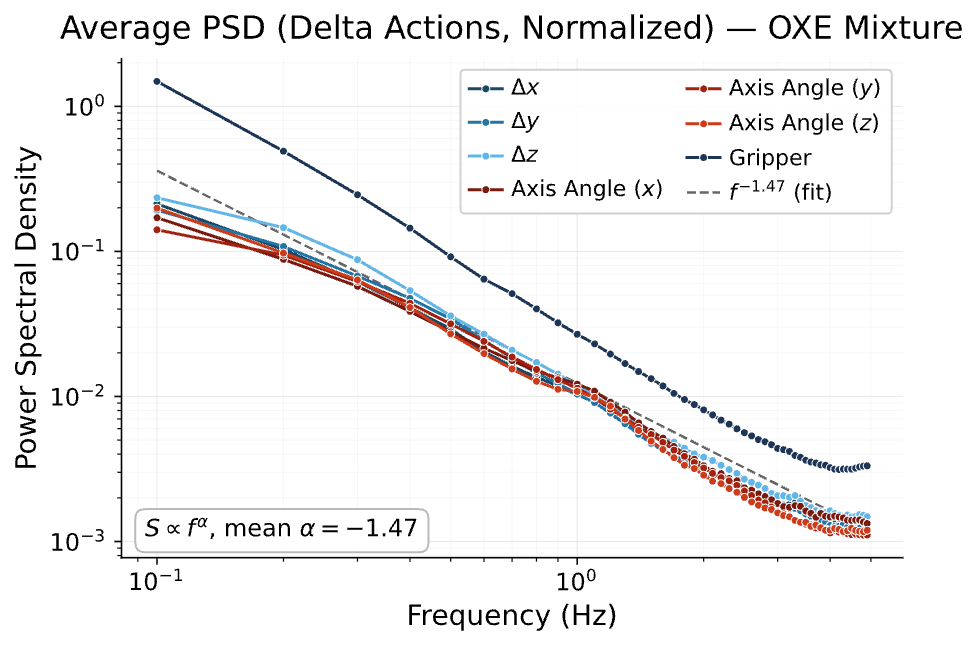
Power Spectral Density (PSD)

https://sander.ai/2024/09/02/spectral-autoregression.html

By Sander Dieleman

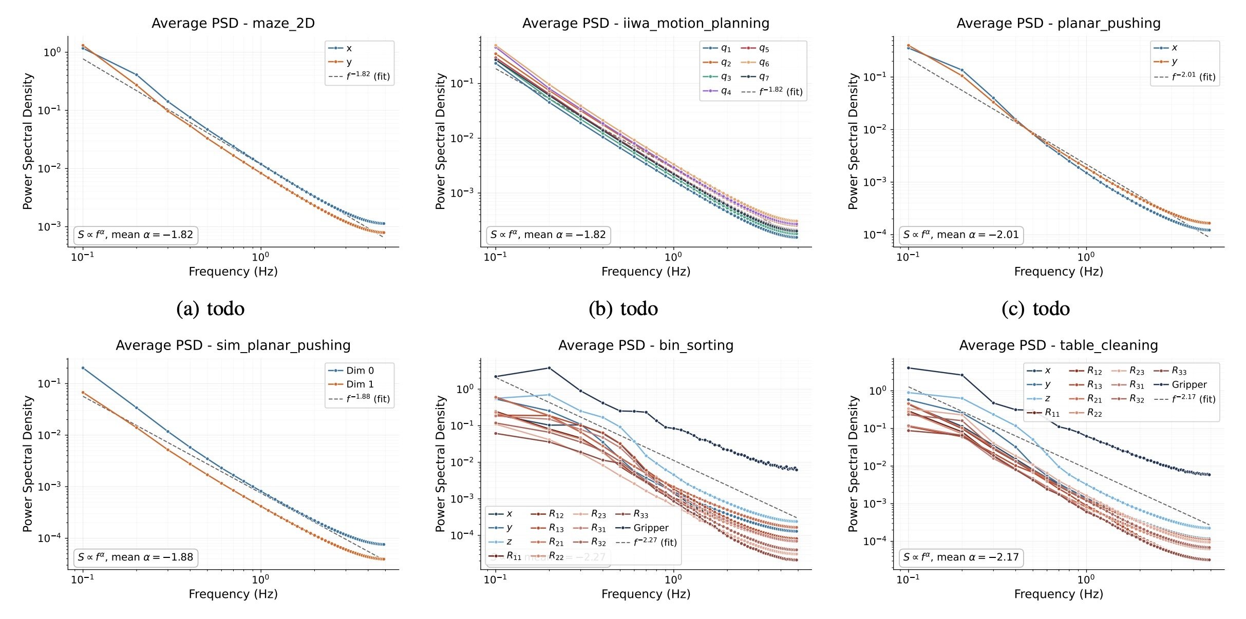
Image data has spectral power law

\(\implies\)

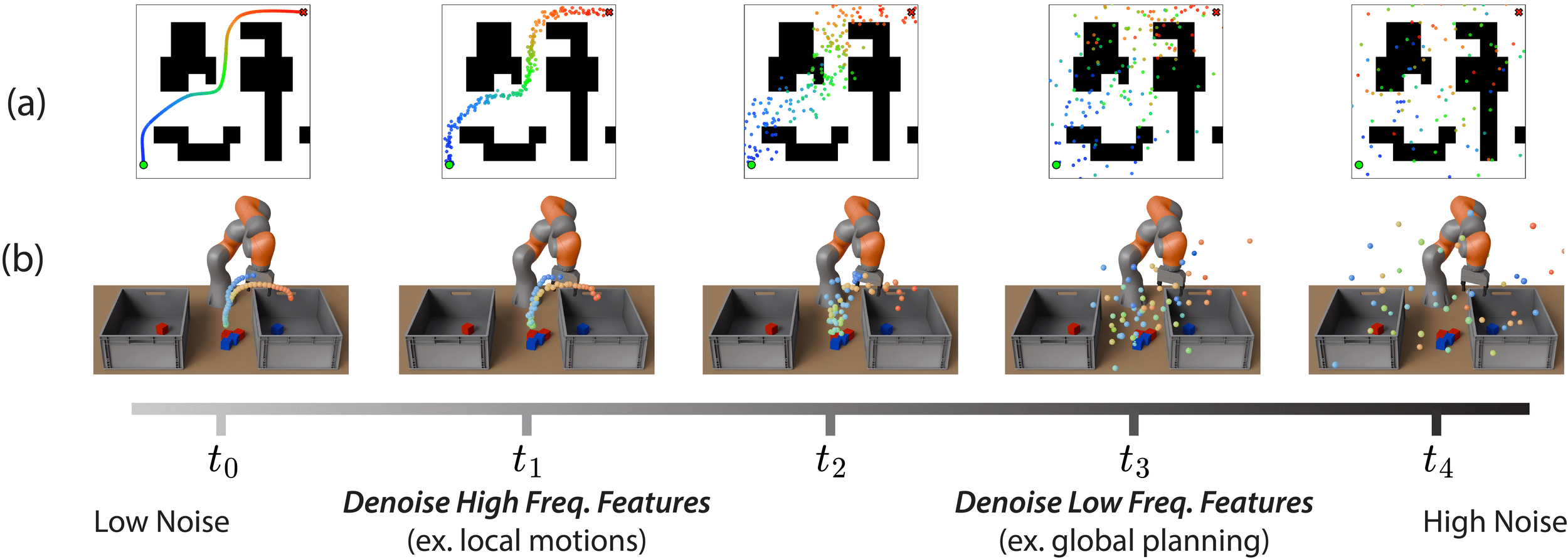
Image diffusion is coarse-to-fine
Noise masks high-freq first

Robot action data exhibits a spectral power law

Loss Function

Loss Function (for \(x_0\sim q_0\))

Denoising Loss vs Ambient Loss

Robot Data: PSD

Loss Function

Loss Function (for \(x_0\sim q_0\))

Denoising Loss vs Ambient Loss

Robot Data: PSD

Loss Function

Loss Function (for \(x_0\sim q_0\))

Denoising Loss vs Ambient Loss

Implications for Robotics

Loss Function

Loss Function (for \(x_0\sim q_0\))

Denoising Loss vs Ambient Loss

Implications for Robotics

Loss Function

Loss Function (for \(x_0\sim q_0\))

Denoising Loss vs Ambient Loss

Implications for Diffusion Policy

Loss Function

Loss Function (for \(x_0\sim q_0\))

Denoising Loss vs Ambient Loss

1. Implications for Diffusion Policy

Diffusion Policy's learn different features at different noise levels

We should only use suboptimal data when it aligns with high-quality data

Loss Function

Loss Function (for \(x_0\sim q_0\))

Denoising Loss vs Ambient Loss

2. Implications for Ambient Diffusion Policy

Noise masks motion primitives first

\(\implies t_{min}\) is small when the suboptimality is motion-level

Noise masks motion primitives first

\(\implies t_{min}\) is small when the suboptimality is motion-level

i.e. \(q\) contains the correct global plan, but the incorrect low-level motions

Noisy or non-expert teleop
Sim2real gaps
Changes in low-level controller

Embodiment gap
Hand-tracking Data
Different environment, objects, etc

2. Implications for Ambient Diffusion Policy

Loss Function

Loss Function (for \(x_0\sim q_0\))

Denoising Loss vs Ambient Loss

Ambient Diffusion Policy

\(t_{\min}\)

\(t> t_{\min}\)

"High-quality" Data

\(t=T\)

For all \(t \in [0,T]\): train \(h_\theta(A_t, O, t) \approx \mathbb{E}[A_0 \mid A_t, O]\)

\(t<t_{\max}\)

\(t_{\max}\)

\(p_t\) \(\approx\) \(q_t\)

"Locality"

Both intervals \([0, t_{max})\) and \((t_{min}, T]\) have interpretations.

\(t=0\)

Loss Function

Loss Function (for \(x_0\sim q_0\))

Denoising Loss vs Ambient Loss

Task-level Corruptions

What if the action corruption is task-level?

Red \(\rightarrow\) Left

Blue \(\rightarrow\) Right

Red \(\rightarrow\) Right

Blue \(\rightarrow\) Left

(out-dated video...)

Loss Function

Loss Function (for \(x_0\sim q_0\))

Denoising Loss vs Ambient Loss

Locality

Locality (of the optimal denoiser at low noise)

The output at each coordinate depends primarily on a small receptive field in the noisy input

Loss Function

Loss Function (for \(x_0\sim q_0\))

Denoising Loss vs Ambient Loss

Locality

Sensitivity of \(\hat a_0^{(8)}\) to \(a_\sigma^{i}\) at different noise levels

Loss Function

Loss Function (for \(x_0\sim q_0\))

Denoising Loss vs Ambient Loss

Locality

Locality (of the optimal denoiser at low noise)

The output at each coordinate depends primarily on a small receptive field in the noisy input

For robotics, denoisers at low noise

Learn motion primitives
Ignore global task structure

\(\implies\) can learn to grasp from data for the wrong task!

Part 4a

Controlled Experiments

Question break!

Ambient Diffusion Policy

\(t_{\min}\)

\(t> t_{\min}\)

"High-quality" Data

\(t=T\)

For all \(t \in [0,T]\): train \(h_\theta(A_t, O, t) \approx \mathbb{E}[A_0 \mid A_t, O]\)

\(t_{\max}\)

\(p_t\) \(\approx\) \(q_t\)

\(t=0\)

Following 3 experiments only use \(t_{min}\)

Loss Function

Loss Function (for \(x_0\sim q_0\))

Denoising Loss vs Ambient Loss

Choosing \(\sigma_{min}\)

Motion Planning Experiments

Distribution shift: Low-quality, noisy trajectories

High Quality:

100 GCS trajectories

Low Quality:

5000 RRT trajectories

Loss Function

Loss Function (for \(x_0\sim q_0\))

Denoising Loss vs Ambient Loss

Choosing \(\sigma_{min}\)

Task vs Motion Level

Distribution shift: Low-quality, noisy trajectories

\(\sigma=0\)

5000 RRT Trajectories

\(\sigma_{min}\)

\(\sigma=1\)

100 GCS Trajectories

Task level:

learn the maze structure

Motion level:

learn smooth motions

Loss Function

Loss Function (for \(x_0\sim q_0\))

Denoising Loss vs Ambient Loss

Choosing \(\sigma_{min}\)

Results

GCS

Success Rate

Avg. Acc^2

(Motion-level)

RRT

GCS+RRT

(Co-train)

GCS+RRT

(Ambient)

57.5%

Swept for best \(t_{min}\) per dataset

Policies evaluated over 1000 trials each

99.0%

141.65

74.8

99.4%

62.2

99.5%

30.9

Loss Function

Loss Function (for \(x_0\sim q_0\))

Denoising Loss vs Ambient Loss

Choosing \(\sigma_{min}\)

Qualitative Results

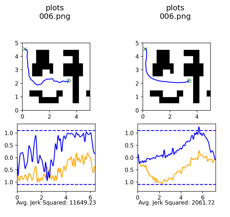
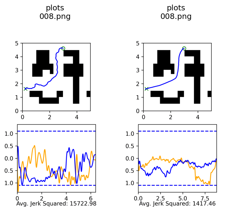
Co-trained

Ambient

Loss Function

Loss Function (for \(x_0\sim q_0\))

Denoising Loss vs Ambient Loss

Choosing \(\sigma_{min}\)

7-DoF Motion Planning

Clean data:

100k trajopt trajectories

Corrupt data:

1M RRT trajectories

Loss Function

Loss Function (for \(x_0\sim q_0\))

Denoising Loss vs Ambient Loss

Choosing \(\sigma_{min}\)

7-DoF Motion Planning

Trajopt

Success Rate

Avg. Acc^2

(Motion-level)

RRT

Trajopt+RRT

(Co-train)

Trajopt+RRT

(Ambient)

46.0%

52.0%

3.9

54.9

59.9%

42.7

65.9%

31.4

Swept for best \(\sigma_{min}\) per dataset

Policies evaluated over 1000 trials each

Sim & Real Cotraining

Distribution shift: sim2real gap

In-Distribution:

50 demos in "target" environment

Out-of-Distribution:

2000 demos in sim environment

Loss Function

Loss Function (for \(x_0\sim q_0\))

Denoising Loss vs Ambient Loss

Choosing \(\sigma_{min}\)

Results

"Real" Only

Success Rate

Co-train

Ambient

(single \(t_{min}\))

56.5%

Policies evaluated over 200 trials each

84.5%

87.0%

Ambient

(\(t_{min}\) per datapoint)

93.5%

Goal: isolate the effect of locality in robotics

Locality Only

"High-quality" Data

\(t=T\)

For all \(t \in [0,T]\): train \(h_\theta(A_t, O, t) \approx \mathbb{E}[A_0 \mid A_t, O]\)

\(t<t_{\max}\)

\(t_{\max}\)

"Locality"

\(t=0\)

Example: Bin Sorting

Distribution shift: task level mismatch, motion level correctness

In-Distribution:

50 demos with correct sorting logic

Out-of-Distribution:

200 demos with incorrect sorting

Metrics

Robot needs to learn two things:

1. Motion Planning

2. Logic

\(\frac{\#\ blocks \ in \ any \ bin}{total \ blocks}\)

\(\frac{\# \ blocks \ in \ correct \ bin}{\# \ blocks \ \ in \ any bin}\)

Goal: learn motion planning from the bad data, but not the task planning

Success rate:

\(\frac{\# \ blocks \ in \ correct \ bin}{\# \ total \ blocks}\) = (motion planning) x (logic)

Results

Diffusion

Success Rate

Logic Metric

Cotrain

Motion Metric

Locality

61.0%

61.9%

98.6%

22.7%

87.2%

26.0%

93.3%

95.0%

98.2%

Task Planning

Motion Planning

Task Conditioning

Success Rate

Logic Metric

Cotrain

(with task condition)

Motion Metric

Locality

90.3%

91.5%

98.6%

93.3%

95.0%

98.2%

Locality

(with task condition)

92.8%

94.2%

98.5%

Part 4b

Scaling Experiments

Scaling to Real-World Datasets

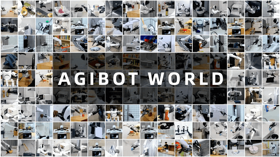
Open-X

Diffusion Policy

In-Distribution Data

Policy

\(\pi(a | o, l)\)

\(p\)

\(q\)

"Suboptimal" / OOD Data

cross-embodied
diff. teleoperators
sim data

mislabeled data
diff tasks, environments, camera

"Suboptimal" Data

Open-X

Magic Soup++: 27 Datasets

Custom OXE: 48 Datasets

1.4M episodes
55M "datagrams"

Table Cleaning

Tower Building

*both videos are autonomous rollouts from Ambient Diffusion Policies at 2x speed

Table Cleaning & Tower Building

Scaling to Real-World Datasets

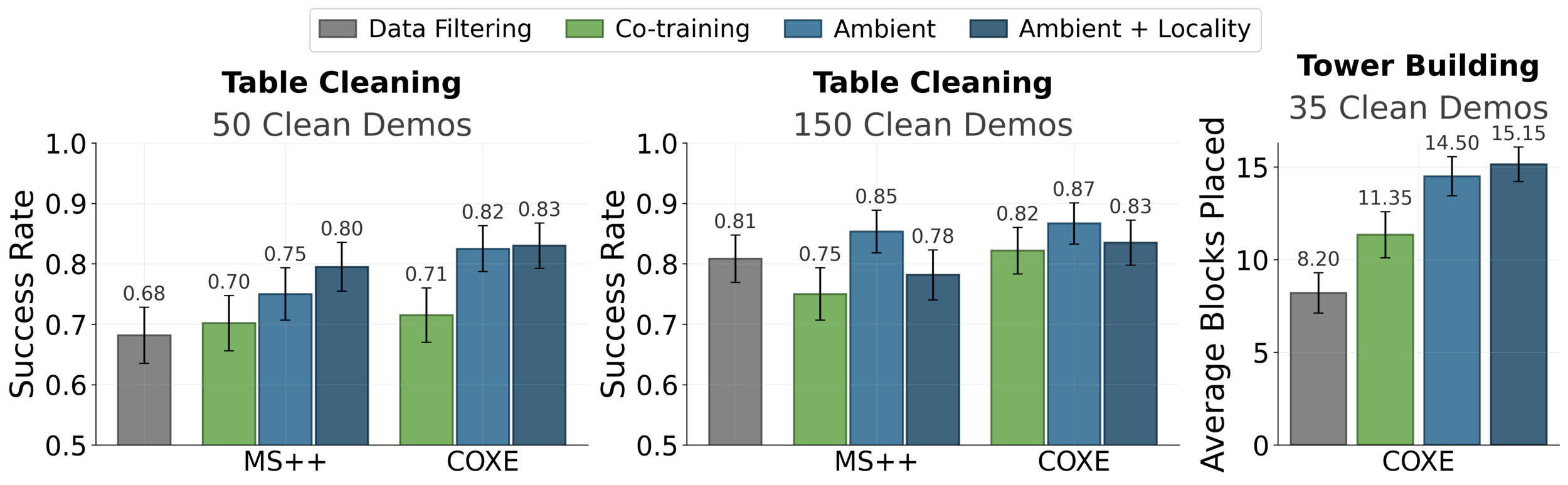
84%

33%

More "suboptimal" data

Ablations

Finetuning comparison
Re-weighting + Ambient
"Suboptimal" Observations
Parameter sweeps
Evidence of global-to-local hierarchy

Part 5

Limitations and Future Work

Future Directions

Q: What is "in-distribution" or "high-quality"?

A [in this paper]: expert teleoperator on your robot, your task, your environment

A [more generally]: data quality?

Q: Better methods to choose \(t_{min}\) and \(t_{max}?\)

Q: Soft Ambient / Rejection-based sampling

Thank You!

Ambient can be used to learn from any suboptimal / OOD data in robotics

In-Distribution Data

Open-X

simulation

Suboptimal / OOD Data

Paper link: will arXiv soon! (likely Tuesday night)