Cotraining for Diffusion Policies
Oct 25, 2024
Adam Wei
Congratulations Dr. Terry Suh!

🎉

🎉
It's ok Terry :(
PhD
❌
Start Up
✅
Screw the PhD...
Mr. Suh sounded better anyways...

Agenda
- Motivation
- Cotraining & Problem Formulation
- Vanilla Cotraining & Insights
- Algorithms for cotraining
- Future Work
Motivation: Sim Data
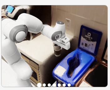
Sim Infrastructure
Sim Data Generation

Motivation: Sim Data
- Simulated data is here to stay => we should understand how to use this data...
- Best practises for training from heterogeneous datasets is not well understood (even for real only)
Octo
DROID
Similar comments in OpenX, OpenVLA, etc...
Motivation: High-level Goals
... will make more concrete in a few slides
- Empirical sandbox results to inform cotraining practises
- Understand the qualities in sim data that affect performance
- Propose new algorithms for cotraining
Problem Formulation
Robot Actions
O
A

Robot Actions
A
O
Ex: From a human demonstrator
Ex: From GCS
Problem Formulation
Robot Actions
O
A
Robot Actions
A
O
- High quality data from the target distribution
- Expensive to collect
- Not the target distribution, but still informative data
- Scalable to collect
Problem Formulation
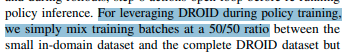
Cotraining: Use both datasets to train a model that maximizes some test objective
- Model: Diffusion Policy that learns \(p(A|O)\)
- Test objective: Empirical success rate on a planar pushing task
Notation
R, S => real and sim
\(|\mathcal D|\) = # demos in \(\mathcal D\)
\(\mathcal{L}=\mathbb{E}_{p_{O,A},k,\epsilon^k}[\lVert \epsilon^k - \epsilon(O_t, A^o_t + \epsilon^k, k) \rVert^2] \)
\(\mathcal{L}_{\mathcal{D}}=\mathbb{E}_{\mathcal{D},k,\epsilon^k}[\lVert \epsilon^k - \epsilon(O_t, A^o_t + \epsilon^k, k) \rVert^2] \approx \mathcal L \)
\(\mathcal D^\alpha\) Dataset mixture
- Sample from \(\mathcal D_R\) w.p. \(\alpha\)
- Sample from \(\mathcal D_S\) w.p, \(1-\alpha\)
Research Questions
- For vanilla cotraining: how do \(|\mathcal D_R|\), \(|\mathcal D_S|\), and \(\alpha\) affect the policy's success rate?
- How do distribution shifts affect cotraining?
- Propose new algorithms for cotraining
- Adversarial formulation
- Classifier-free guidance
Informs the qualities we want in sim
Vanilla Cotraining
(Tower property of expectations)
Instead:
- Choose \(\alpha \in [0,1]\)
- Train a diffusion policy that minimizes \(\mathcal L_{\mathcal D^\alpha}\)
Experiments
For vanilla cotraining: how do \(|\mathcal D_R|\), \(|\mathcal D_S|\), and \(\alpha\) affect the policy's success rate?
- Distributionally robust optimization, Re-Mix, etc
- Theoretical bounds
- Empirical approach
Experiment Setup
\(|\mathcal D_R|\) = 10, 50, 150 demos
\(|\mathcal D_S|\) = 500, 2000 demos
\(\alpha = 0,\ \frac{|\mathcal{D}_{R}|}{|\mathcal{D}_{R}|+|\mathcal{D}_{S}|},\ 0.25,\ 0.5,\ 0.75,\ 1\)
Sweep the following parameters:
For vanilla cotraining: how do \(|\mathcal D_R|\), \(|\mathcal D_S|\), and \(\alpha\) affect the policy's success rate?
Experiment Setup
- Train for ~2 days on a single Supercloud V100
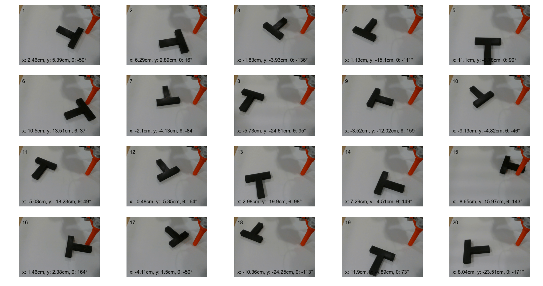
- Evaluate performance on 20 trials from matched initial conditions
Results
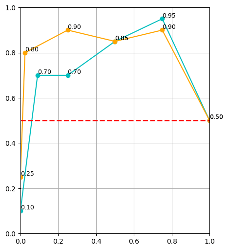

\(|\mathcal D_R| = 10\)
\(|\mathcal D_R| = 50\)
\(|\mathcal D_R| = 150\)
cyan: \(|\mathcal D_S| = 500\) orange: \(|\mathcal D_S| = 2000\) red: real only
Takeaways: \(\alpha\)
- Policy's are sensitive to \(\alpha\), especially when \(|\mathcal D_R|\) is small
- Smaller \(|\mathcal D_R|\) → smaller \(\alpha\)
- Larger \(|\mathcal D_R|\) → larger \(\alpha\)
- If \(|\mathcal D_R|\) is sufficiently large, sim data will not help. It also isn't detrimental.
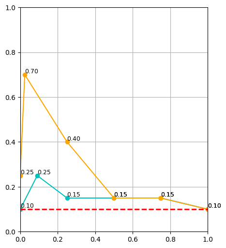
Results
\(|\mathcal D_R| = 10\)
\(|\mathcal D_R| = 50\)
\(|\mathcal D_R| = 150\)
cyan: \(|\mathcal D_S| = 500\) orange: \(|\mathcal D_S| = 2000\) red: real only
Takeaways: \(|\mathcal D_R|\), \(|\mathcal D_S|\)
- Cotraining improves policy performance at all data scales
- Scaling \(|\mathcal D_S|\) improves performance. This effect is drastically more pronouced for small \(|\mathcal D_R|\)
- Scaling \(|\mathcal D_S|\) reduces sensitivity of \(\alpha\)
Initial experiments suggest that scaling up sim is a good idea!
... to be verified at larger scales with sim-sim experiments
Cotraining Theory
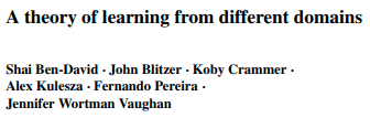

Cotraining Theory
\(|\mathcal D_R|\)
\(|\mathcal D_S|\)
Experiments match intuition and theoretical bounds
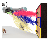
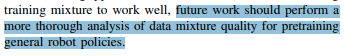
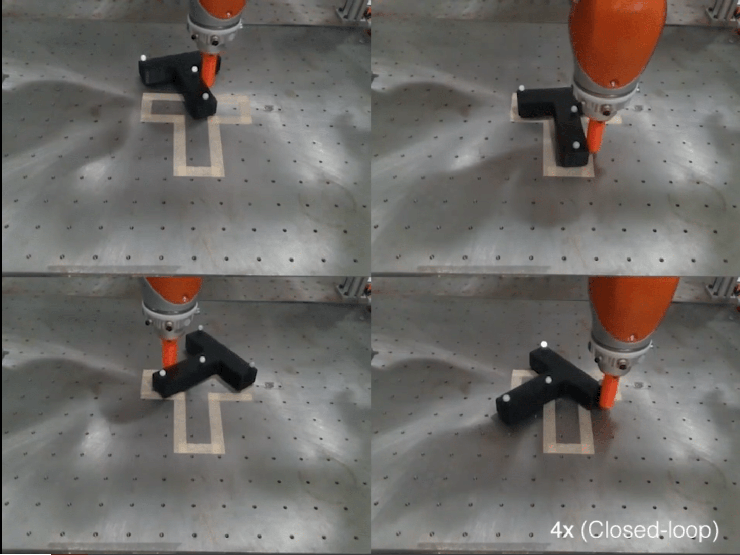
How does cotraining help?
Sim Demos
Real Rollout
see other tab
Cotrained Policies
Cotrained policies exhibit similar characteristics to the real-world expert regardless of the mixing ratio
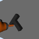
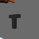
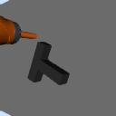
Real Data
- Aligns orientation, then translation sequentially
- Sliding contacts
- Leverage "nook" of T
Sim Data
- Aligns orientation and translation simultaneously
- Sticking contacts
- Pushes on the sides of T
How does cotraining improve performance?
Hypothesis
- When deployed in real, cotrained policies rely on real data and use sim data to fill in the gaps
- Sim data prevents overfitting and acts as a regularizor
- Sim data provides more information about high probability actions \(p_A(a)\)
Probably some combination of the above.
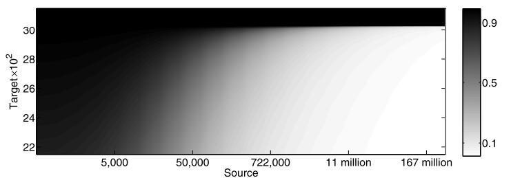
Hypothesis 1: Binary classification
When deployed in real, cotrained policies rely on real data and use sim data to fill in the gap
| Policy | Observation embeddings acc. | Final activation acc. |
|---|---|---|
| 50/500, alpha = 0.75 | 100% | 74.2% |
| 50/2000, alpha = 0.75 | 100% | 89% |
| 10/2000, alpha = 0.75 | 100% | 93% |
| 10/2000, alpha = 5e-3 | 100% | 94% |
| 10/500, alpha = 0.02 | 100% | 88% |
Only a small amount of real data is needed to separate the embeddings and activations
Hypothesis 1: tSNE
- t-SNE visualization of the observation embeddings
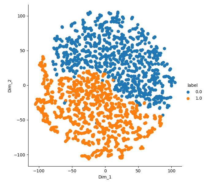
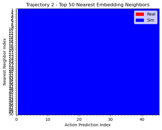
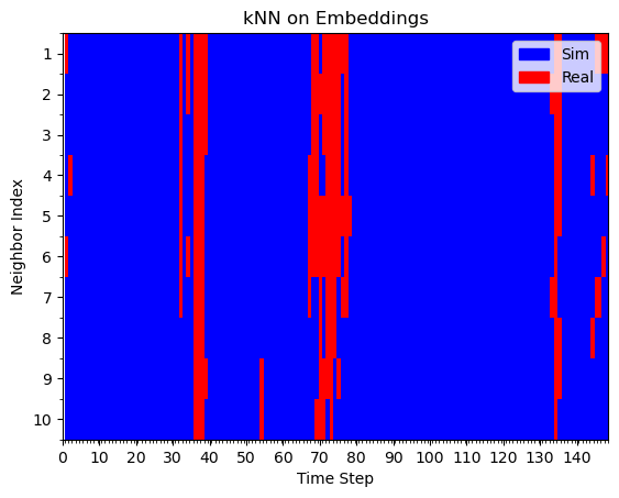
Hypothesis 1: kNN on actions

Real Rollout
Sim Rollout
Mostly red with blue interleaved
Mostly blue
Assumption: if kNN are real/sim, this behavior was learned from real/sim
Similar results for kNN on embeddings
Hypothesis 1: kNN on embeddings
Real Rollout
Sim Rollout
Some red
All blue
Hypothesis 2
Sim data prevents overfitting and acts as a regularizor
When \(|\mathcal D_R|\) is small, \(\mathcal L_{\mathcal D_R}\not\approx\mathcal L\).
\(\mathcal D_S\) helps regularize and prevent overfitting
Hypothesis 3
Sim data provides more information about \(p_A(a)\)
- i.e. improves the cotrained policies prior on "likely actions"
Can we test/leverage this hypothesis with classifier-free guidance?
... more on this later if time allows
Hypothesis 3
Sim data provides more information about \(p_A(a)\)
Can we leverage this with classifier free guidance...
}
Research Questions
- For vanilla cotraining: how do \(|\mathcal D_R|\), \(|\mathcal D_S|\), and \(\alpha\) affect the policy's success rate?
- How do distribution shifts affect cotraining?
-
Propose new algorithms for cotraining
- Adversarial formulation
- Classifier-free guidance
Informs the qualities we want in sim
Distribution Shifts
Setting up a simulator for data generation is non-trivial
- camera calibration, colors, assets, physics, tuning, data filtering, task-specifications, etc
+ Actions
What qualities matter in the simulated data?
Distribution Shifts

Distribution Shifts
Visual Shifts
- Domain randomization
- Color shift
Physics Shifts
- Center of mass shift
Task Shifts
- Goal Shift
- Object shift


Original
Color Shift
Goal Shift
Object Shift
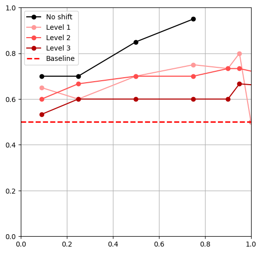
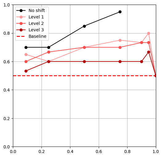
Distribution Shifts
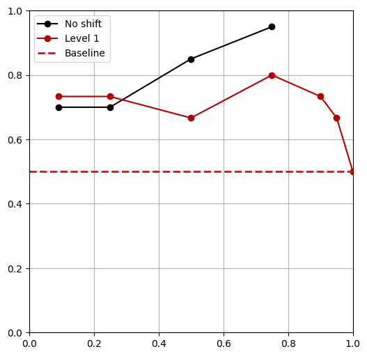
- Tested 3 levels of shift for each shift**
- \(|\mathcal D_R|\) = 50, \(|\mathcal D_S|\) = 500,
- \(\alpha = 0,\ \frac{|\mathcal{D}_{R}|}{|\mathcal{D}_{R}|+|\mathcal{D}_{S}|},\ 0.25,\ 0.5,\ 0.75,\ 0.9,\ 0.95,\ 1\)
** Except object shift
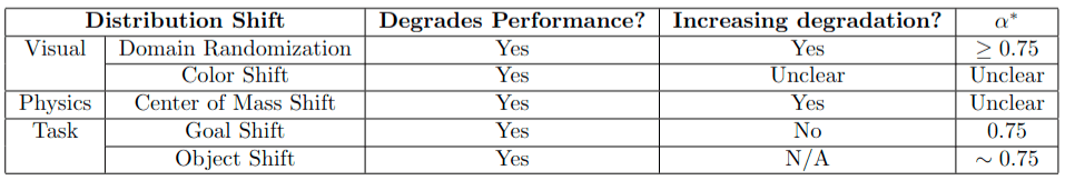
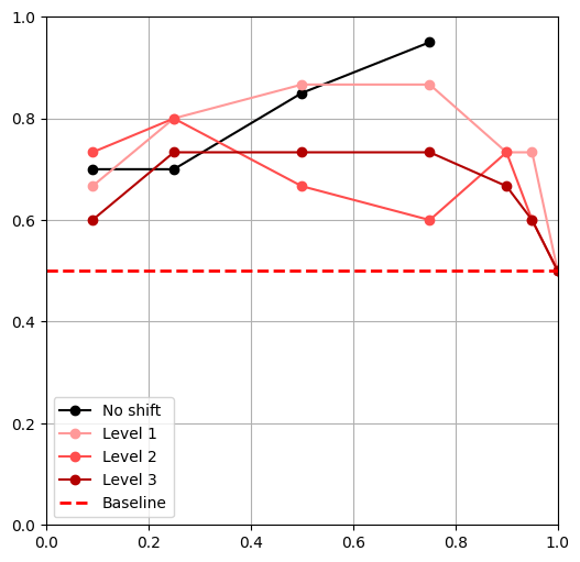
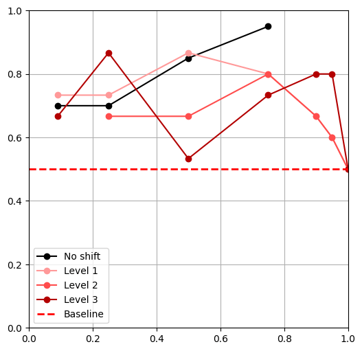
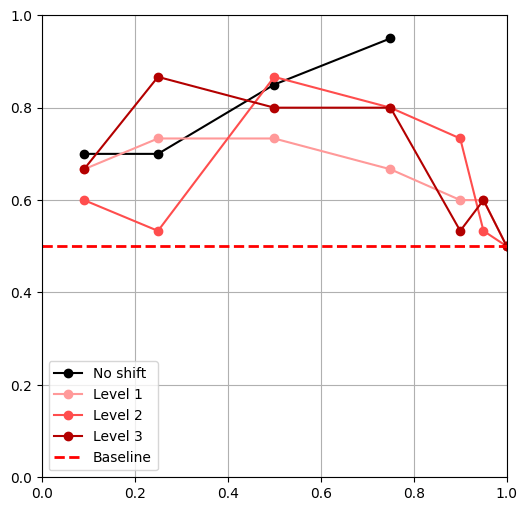
- All policies outperform the 'real only' baseline
Visual Shifts
Domain Randomization
Color Shift
Physics Shifts
Center of Mass Shift

Task Shifts
Goal Shift
Object Shift
Research Questions
- For vanilla cotraining: how do \(|\mathcal D_R|\), \(|\mathcal D_S|\), and \(\alpha\) affect the policy's success rate?
- How do distribution shifts affect cotraining?
- Propose new algorithms for cotraining
- Adversarial formulation
- Classifier-free guidance
Sim2Real Gap
Fact: cotrained models can distinguish sim & real
Thought experiment: what if sim and real were nearly indistinguishable?

Sim2Real Gap
Thought experiment: what if sim and real were nearly indistinguishable?
- Less sensitive to \(\alpha\)
- Each sim data point better approximates the true denoising objective
- Improved zero-shot transfer
- Improved cotraining bounds
Sim2Real Gap
\(\mathrm{dist}(\mathcal D_R,\mathcal D_S)\) small \(\implies p^{real}_{(O,A)} \approx p^{sim}_{(O,A)} \implies p^{real}_O \approx p^{sim}_O\)
'visual sim2real gap'
Sim2Real Gap
Current approaches to sim2real: make sim and real visually indistinguishable
- Gaussian splatting, blender renderings, real2sim, etc
\(p^{R}_O \approx p^{S}_O\)
Do we really need this?
\(p^{R}_O \approx p^{S}_O\)
Sim2Real Gap
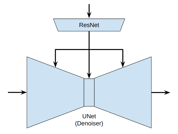
\(a^k\)
\(\hat \epsilon^k\)
\(o \sim p_O\)
\(o^{emb} = f_\psi(o)\)
\(p^{R}_O \approx p^{S}_O\)
\(p^{R}_{emb} \approx p^{S}_{emb}\)
\(\implies\)
Weaker requirement
Adversarial Objective
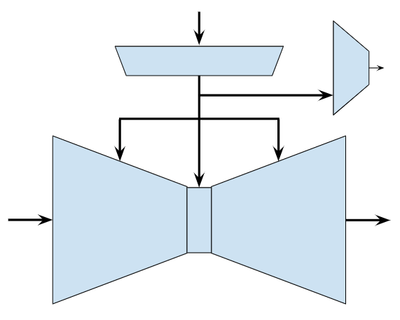
\(\epsilon_\theta\)
\(f_\psi\)
\(d_\phi\)
\(\hat{\mathbb P}(f_\psi(o)\ \mathrm{is\ sim})\)
\(\epsilon^k\)
\(a^k\)
o
Adversarial Objective
Denoiser Loss
Negative BCE Loss
\(\iff\)
(Variational characterization of f-divergences)
thanks Yury! :D
Adversarial Objective
Common features (sim & real)
- End effector position
- Object keypoints
- Contact events
Distinguishable features*
- Shadows, colors, textures, etc
Relavent for controls...
- Adversarial objective discourages the embeddings from encoding distinguishable features*
* also known as protected variables in AI safety literature
Adversarial Objective
Hypothesis:
- Less sensitive to \(\alpha\)
- Less sensitive to visual distribution shifts
- Improved performance for \(|\mathcal D_R|\) = 10
Initial Results
\(|\mathcal D_R| = 50\), \(|\mathcal D_S| = 500\), \(\lambda = 1\), \(\alpha = 0.5\)
Performance: 9/10 trials
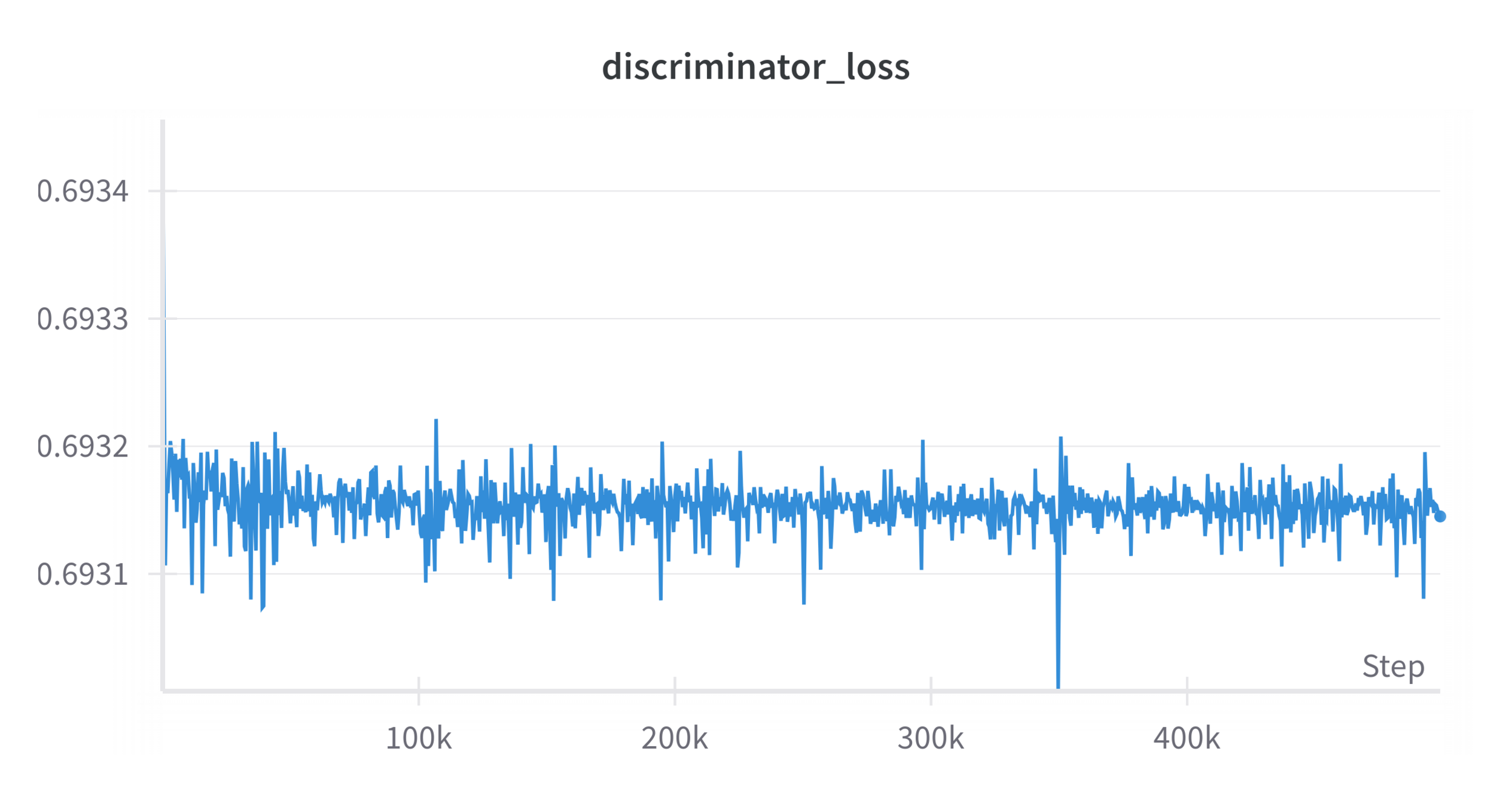
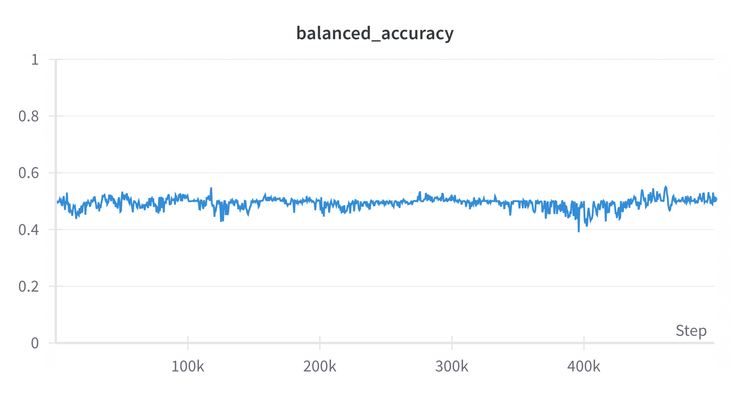
~log(2)
~50%
Problems...
-
A well-trained discriminator can still distinguish sim & real
- This is an issue with the GAN training process (during training, the discriminator cannot be fully trained)
- Image GAN models suffer similar problems
Potential solution?
- Place the discriminator at the final activation?
- Wasserstein GANs (WGANs)
Two Philosophies For Cotraining
1. Minimize sim2real gap
- Pros: better bounds, more performance from each data point
- Cons: Hard to match sim and real, adversarial formulation assumes protected variables are not relevant for control
2. Embrace the sim2real gap
- Pros: policy can identify and adapt strongly to its target domain at runtime, do not need to match sim and real
- Cons: Doesn't enable "superhuman" performance, potentially less data efficient
Hypothesis 3
Sim data provides more information about \(p_A(a)\)
- Sim data provides a strong prior on "likely actions" =>improves the performance of cotrained policies
We can explicitly leverage this prior using classifier free guidance
Conditional Score Estimate
Unconditional Score Estimate
Helps guide the diffusion process
Classifier-Free Guidance
Conditional Score Estimate
- Term 2 guides conditional sampling by separating the conditional and unconditional action distributions
- In image domain, this results in higher quality conditional generation

Difference in conditional and unconditional scores
Classifier-Free Guidance
- Due to the difference term, classifier-free guidance embraces the differences between \(p^R_{(A|O)}\) and \(p_A\)
- Note that \(p_A\) can be provided scalably by sim and also does not require rendering observations!
Future Work
- Finish evaluating finetuned models
- Continue experimenting with adversarial formulations
- Implement and test classifier-free guidance ideas
Immediate next steps:
Future work:
- Sim-sim scaling laws