Learning From Bad Data In Robotics
Sept 26, 2025
Adam Wei
Agenda
- Interpretations
- Motion planning experiments
- Sim-and-real cotraining
- Scaling up "low-quality" data
- Ambient Omni (locality)
- Concluding thoughts
Part 1
Interpretations of Ambient Diffusion
What can go wrong in [CV] data?
CC12M: 12M+ image + text captions

"Corrupt" Data:
Low quality images
"Clean" Data:
High quality images
Not just in CV: also in language, audio, robotics!

Distribution Shifts in Robot Data
- Sim2real gaps
- Noisy/low-quality teleop
- Task-level mismatch
- Changes in low-level controller
- Embodiment gap
- Camera models, poses, etc
- Different environment, objects, etc
robot teleop
simulation

Open-X
Training on OOD Data
robot teleop
simulation
Open-X
There is still value and utility in this data!
... we just aren't using it correctlty
Goal: to develop principled algorithms that change the way we use low-quality or OOD data
"The Present"
2025
"Ambient diffusion is best in domains where good data is hard to get, but bad data is easy"
- i.e. robotics?
"low data"
robot teleop
simulation
Open-X
"The Future"
2025
My bets:
"low data"
1. Robot data will be plentiful
- Ex. Danny Driess (PI)
2. High quality data is hard to get
\(\implies\) this problem will remain relevant
202[?]
"big data"
Loss Function
Loss Function (for \(x_0\sim q_0\))
Denoising Loss vs Ambient Loss
Ambient Diffusion
Repeat:
- Sample \(\sigma\) ~ Unif([0,1])
- Sample (O, A, \(\sigma_{min}\)) ~ \(\mathcal{D}\) s.t. \(\sigma > \sigma_{min}\)
- Optimize denoising loss or ambient loss
\(\sigma=0\)
\(\sigma>\sigma_{min}\)
\(\sigma_{min}\)
*\(\sigma_{min} = 0\) for all clean samples
\(\sigma=1\)
Loss Function (for \(x_0\sim q_0\))
\(\mathbb E[\lVert h_\theta(x_t, t) + \frac{\sigma_{min}^2\sqrt{1-\sigma_{t}^2}}{\sigma_t^2-\sigma_{min}^2}x_{t} - \frac{\sigma_{t}^2\sqrt{1-\sigma_{min}^2}}{\sigma_t^2-\sigma_{min}^2} x_{t_{min}} \rVert_2^2]\)
Ambient Loss
Denoising Loss
\(x_0\)-prediction
\(\epsilon\)-prediction
(assumes access to \(x_0\))
(assumes access to \(x_{t_{min}}\))
\(\mathbb E[\lVert h_\theta(x_t, t) - x_0 \rVert_2^2]\)
\(\mathbb E[\lVert h_\theta(x_t, t) - \epsilon \rVert_2^2]\)
\(\mathbb E[\lVert h_\theta(x_t, t) - \frac{\sigma_t^2 (1-\sigma_{min}^2)}{(\sigma_t^2 - \sigma_{min}^2)\sqrt{1-\sigma_t^2}}x_t + \frac{\sigma_t \sqrt{1-\sigma_t^2}\sqrt{1-\sigma_{min}^2}}{\sigma_t^2 - \sigma_{min}^2}x_{t_{min}}\rVert_2^2]\)
Terminology
"Good" Data
"Bad" Data
- Clean
- In-distribution
- High-quality
- Corrupt
- Out-of-distribution
- Low-quality
Interpations: The Role of Gaussian Noise
1. Gaussian noise = corruption
- Giannis' presentation
- Mirrors the development of the algorithm
-
"but my corruption isn't Gaussian!
- Feel unnatural...
2. Gaussian noise = contraction
- More general
- Better framework for reasoning about what's going on under the hood
- Less jarring
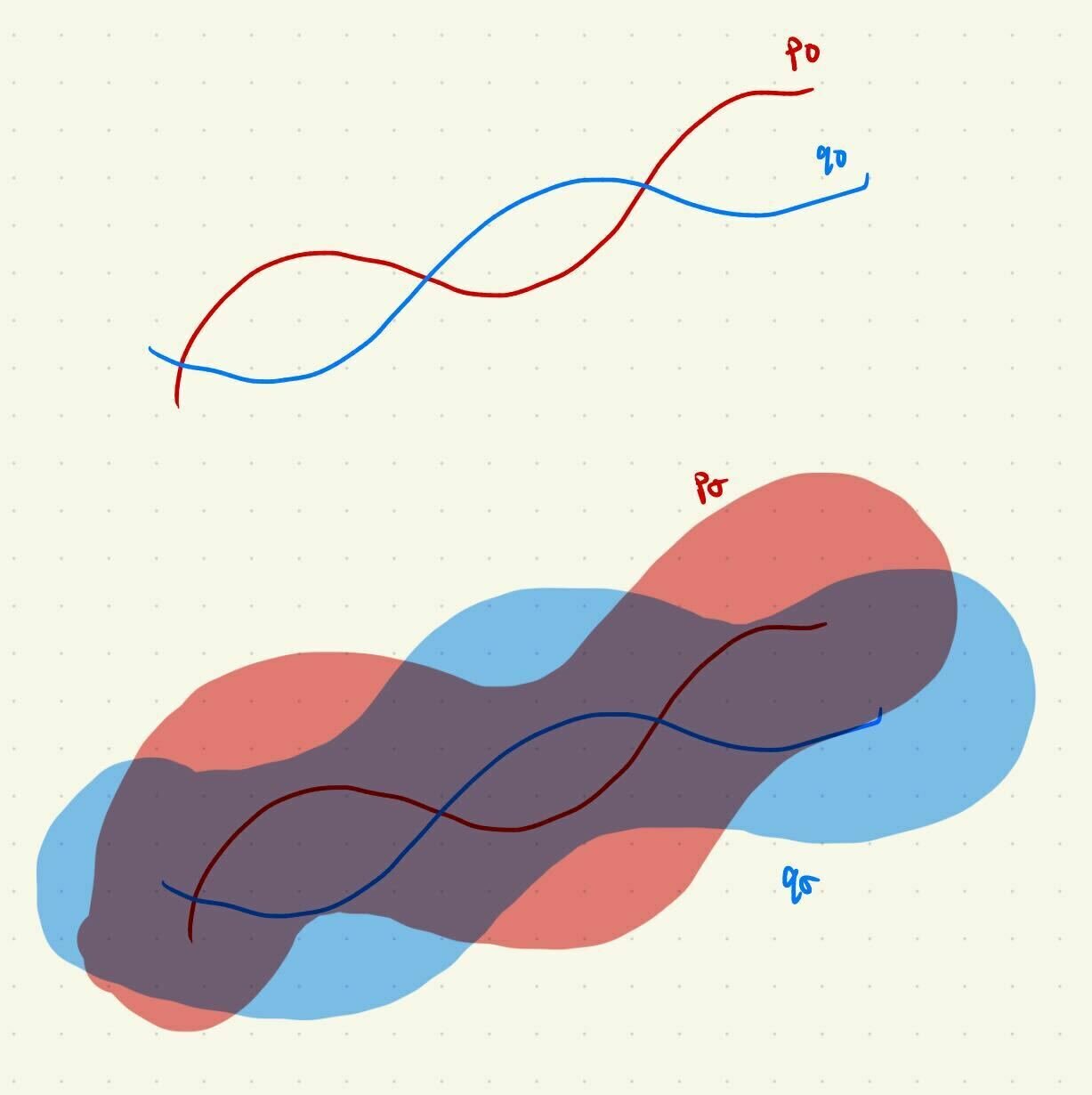
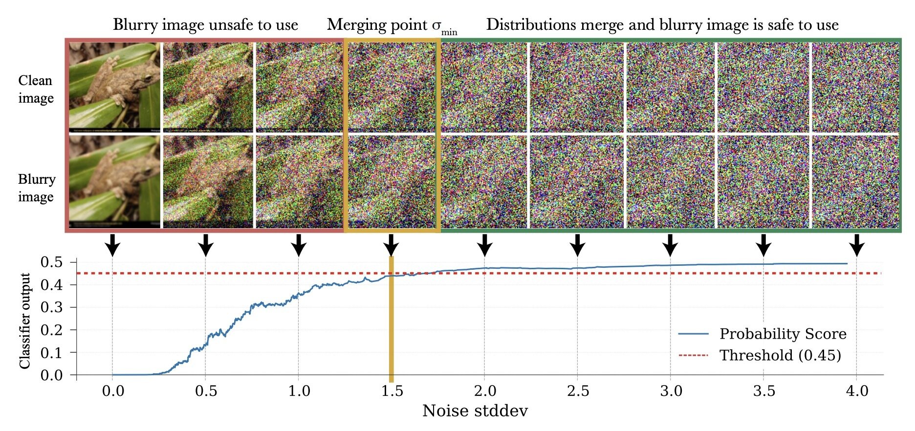
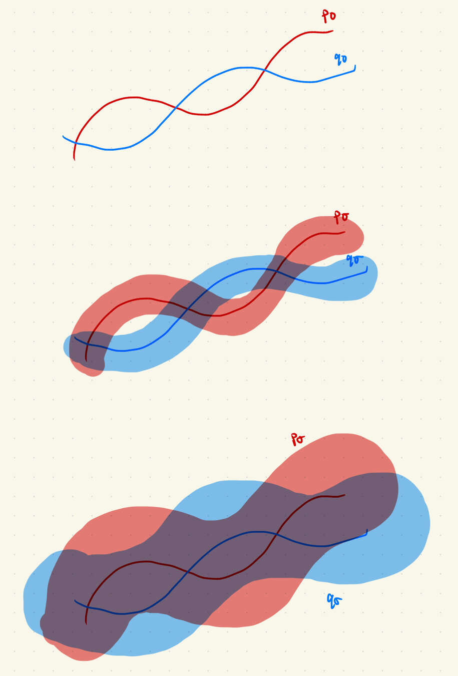
Gaussian Noise As Contraction
\(p_0\)
\(q_0\)
\(p_\sigma\)
\(q_\sigma\)
\(D(p_\sigma, q_\sigma) \to 0\) as \(\sigma\to \infty\)
\(\implies \exists \sigma_{min} \ \mathrm{s.t.}\ D(p_\sigma, q_\sigma) < \epsilon\ \forall \sigma > \sigma_{min}\)
Noisy Channel
\(Y = X + \sigma Z\)
Gaussian Noise As Contraction
\(p_0\)
\(q_0\)
\(p_\sigma=p_0 * \mathcal N(0, \sigma^2\mathrm{I})\)
\(q_\sigma=q_0 * \mathcal N(0, \sigma^2\mathrm{I})\)
1. "Noise as corruption": for \(\sigma > \sigma_{min}\), corruption appears Gaussian
Goal: Learn \(\nabla \log p_\sigma(x)\)
Gaussian Noise As Contraction
\(p_0\)
\(q_0\)
\(p_\sigma=p_0 * \mathcal N(0, \sigma^2\mathrm{I})\)
\(q_\sigma=q_0 * \mathcal N(0, \sigma^2\mathrm{I})\)
Goal: Learn \(\nabla \log p_\sigma(x)\)
2. "Noise as contraction": for \(\sigma > \sigma_{min}\), \(\red{\nabla \log p_\sigma (x)} \approx \blue{\nabla \log q_\sigma (x)}\)
Gaussian Noise As Contraction
Any process that contracts distributions to the same final distribution is viable!
- Ex: Alex's suggestion to noise with a "notch filter"
Different ways to mix the data... more on this later ;)
Noise as contraction: for \(\sigma > \sigma_{min}\), \(\red{\nabla \log p_\sigma (x)} \approx \blue{\nabla \log q_\sigma (x)}\)
Goal: Learn \(\nabla \log p_\sigma(x)\)
Part 2
Motion Planning Experiments
Loss Function
Loss Function (for \(x_0\sim q_0\))
Denoising Loss vs Ambient Loss
Ambient Diffusion
Repeat:
- Sample \(\sigma\) ~ Unif([0,1])
- Sample (O, A, \(\sigma_{min}\)) ~ \(\mathcal{D}\) s.t. \(\sigma > \sigma_{min}\)
- Optimize denoising loss or ambient loss
\(\sigma=0\)
\(\sigma>\sigma_{min}\)
\(\sigma_{min}\)
*\(\sigma_{min} = 0\) for all clean samples
\(\sigma=1\)
Loss Function
Loss Function (for \(x_0\sim q_0\))
Denoising Loss vs Ambient Loss
Choosing \(\sigma_{min}\)
Finding \(\sigma_{min}\)
- Sweep? Use classifier?
Increasing granularity
Assign \(\sigma_{min}\) per datapoint
Assign \(\sigma_{min}\) per dataset
Loss Function
Loss Function (for \(x_0\sim q_0\))
Denoising Loss vs Ambient Loss
Choosing \(\sigma_{min}\)
How to choose \(\sigma_{min}\)?
\(\sigma_{min}^i = \inf\{\sigma\in[0,1]: c_\theta (x_\sigma, \sigma) > 0.5-\epsilon\}\)
\(\implies \sigma_{min}^i = \inf\{\sigma\in[0,1]: d_\mathrm{TV}(p_\sigma, q_\sigma) = 2\epsilon\}\)*
* assuming \(c_\theta\) the best possible classifier
Loss Function
Loss Function (for \(x_0\sim q_0\))
Denoising Loss vs Ambient Loss
Choosing \(\sigma_{min}\)
Motion Planning Experiments
Distribution shift: Low-quality, noisy trajectories
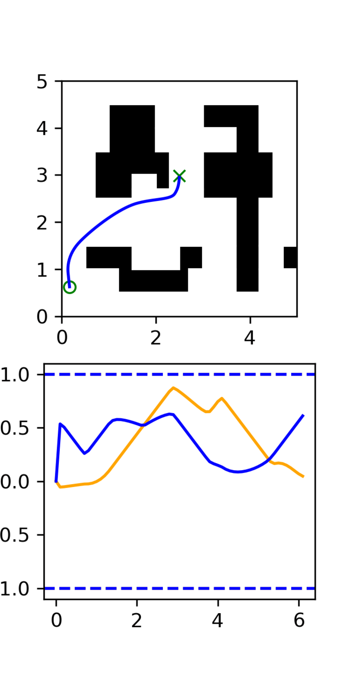
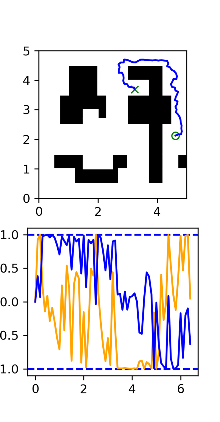
High Quality:
100 GCS trajectories
Low Quality:
5000 RRT trajectories
Note: This experiment is easily generalizable to 7-DoF robot motion planning
Loss Function
Loss Function (for \(x_0\sim q_0\))
Denoising Loss vs Ambient Loss
Choosing \(\sigma_{min}\)
Task vs Motion Level
Distribution shift: Low-quality, noisy trajectories
\(\sigma=0\)
5000 RRT Trajectories
\(\sigma_{min}\)
\(\sigma=1\)
100 GCS Trajectories
Task level:
learn the maze structure
Motion level:
learn smooth motions
Loss Function
Loss Function (for \(x_0\sim q_0\))
Denoising Loss vs Ambient Loss
Choosing \(\sigma_{min}\)
Results
GCS
Success Rate
(Task-level)
Avg. Jerk^2
(Motion-level)
RRT
GCS+RRT
(Co-train)
GCS+RRT
(Ambient)
50%
Swept for best \(\sigma_{min}\) per dataset
Policies evaluated over 100 trials each
100%
7.5k
17k
91%
14.5k
98%
5.5k
Loss Function
Loss Function (for \(x_0\sim q_0\))
Denoising Loss vs Ambient Loss
Choosing \(\sigma_{min}\)
Qualitative Results
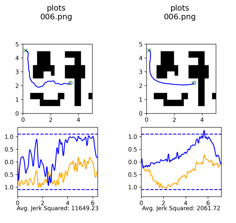
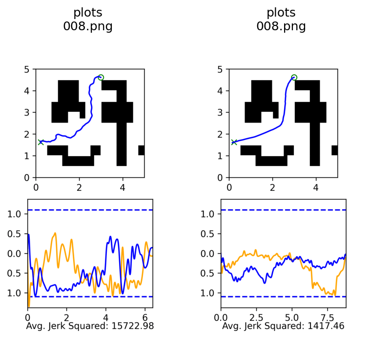
Co-trained
Ambient
Part 3
Sim-and-Real Cotraining
Sim & Real Cotraining
Distribution shift: sim2real gap
In-Distribution:
50 demos in "target" environment
Out-of-Distribution:
2000 demos in sim environment
Experiments
Experiment 1: swept \(\sigma_{min}\) per dataset
Experiment 2: estimated \(\sigma_{min}\) per datapoint with a classifier
Caveat! Classifier was trained to predict sim vs real actions
- ie. trained to distinguish \(p(A)\) and \(q(A)\)
- as opposed to \(p(A|O)\) and \(q(A | O)\)
Experiment 3: exploring ambient diffusion at different data scales
Experiments 1 & 2
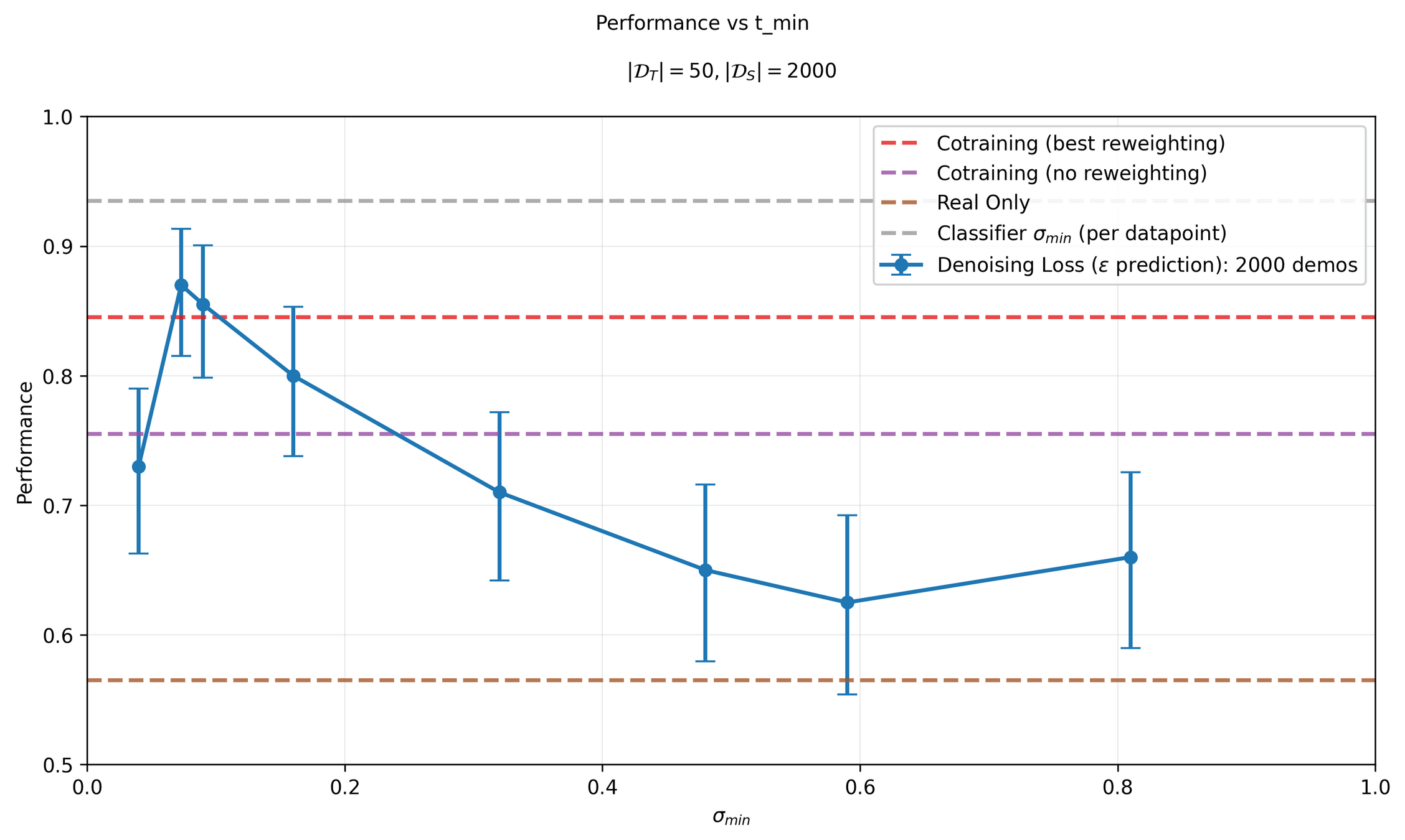
Moving forwards, all experiments will use the classifier
10 Real Demos
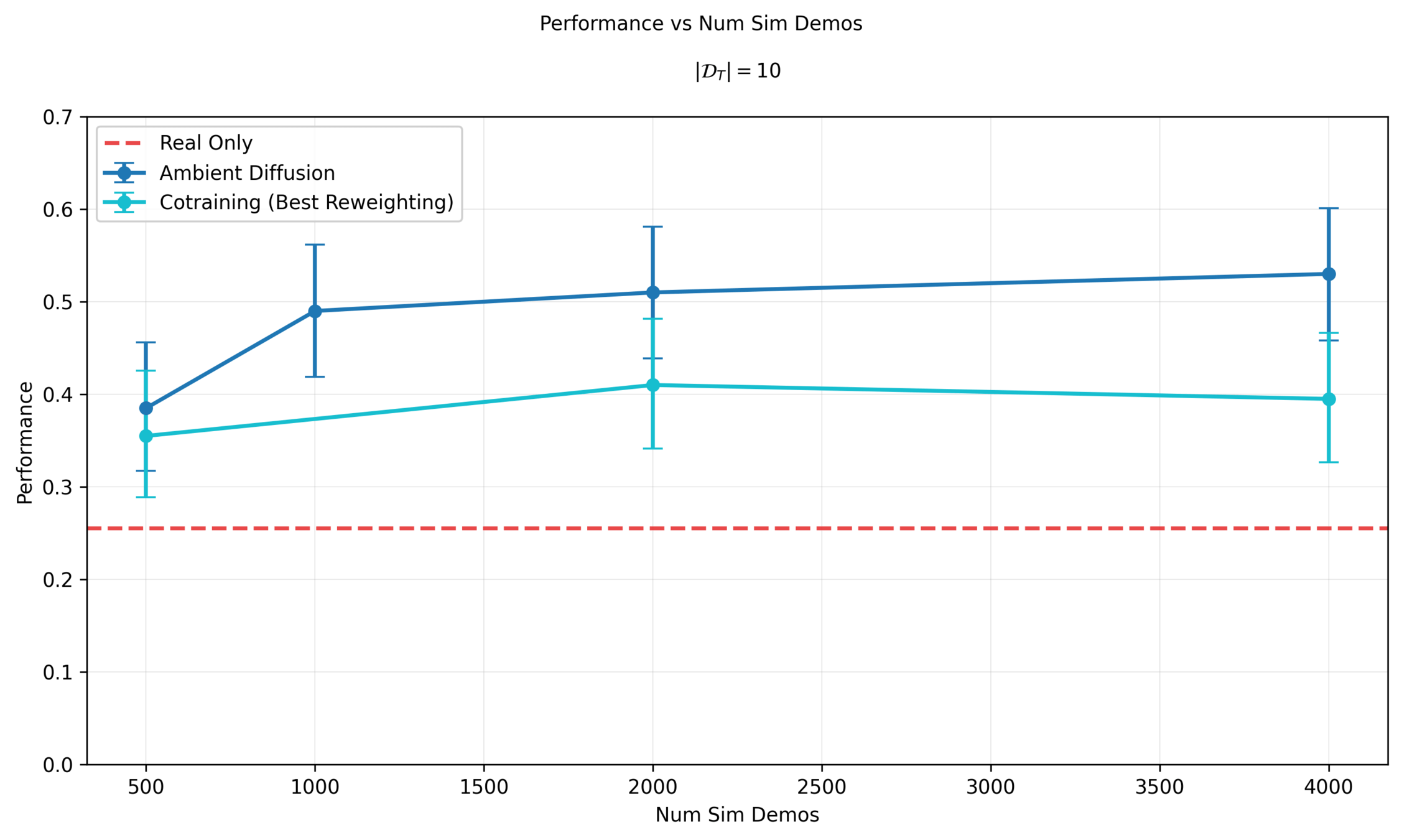
50 Real Demos
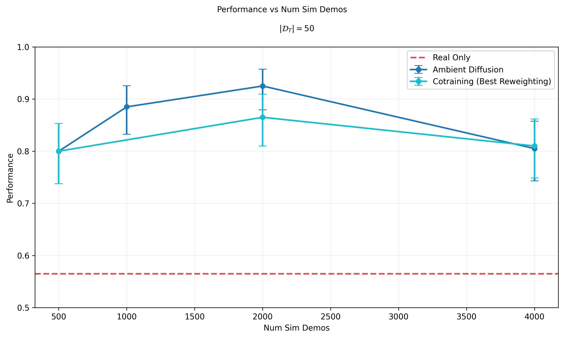
!!
Part 4
Scaling Low-Quality Data
Denoising Loss vs Ambient Loss
Whats going wrong?
Problem 1
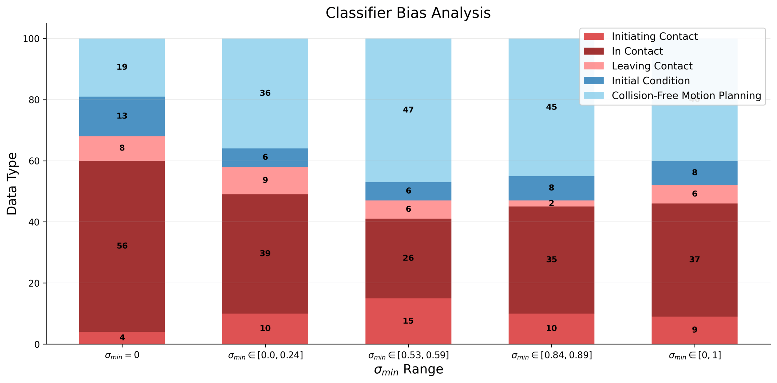
Classifier biases data distribution at different noise-levels
Denoising Loss vs Ambient Loss
What's going wrong?
Let's examine the problems one at a time...
Ambient \(\to\) sim-only as \(|\mathcal{D}_S| \to \infty\)
... and sim-only is bad!
Classifier biases data distribution at different noise-levels
Problem 1
Problem 2
Denoising Loss vs Ambient Loss
Problem 1: Biasing from classifier
Some "types" of data are more likely to be assigned low \(\sigma_{min}\)
- This biases the training distribution, and thus the sampling distribution
Denoising Loss vs Ambient Loss
Thought Experiment
\(q_0\) =
w.p. \(\frac{1}{2}\)
w.p. \(\frac{1}{2}\)
\(p_0\) =
w.p. \(\frac{1}{2}\)
w.p. \(\frac{1}{2}\)
Denoising Loss vs Ambient Loss
Thought Experiment
\(q_0\) =
w.p. \(\frac{1}{2}\)
w.p. \(\frac{1}{2}\)
- Training becomes biased towards dogs
- In the limit of \(\infty\) samples from \(q_0\), we will only generate dogs!!
not in \(p_0\)
\(\implies\) \(\sigma_{min}\approx 1\)
(dont use this data)
in \(p_0\)
\(\implies\) \(\sigma_{min}\approx 0\)
(use this data!)
Denoising Loss vs Ambient Loss
Is Problem 1 real?
Mode 1
Mode 2
Mode 3
Mode 4
Denoising Loss vs Ambient Loss
Is Problem 1 real?
Mode 1
Mode 2
Mode 3
Mode 4
Denoising Loss vs Ambient Loss
Solution: Bucketing
"Can't do statistics with n=1" - Costis
Increasing granularity
Assign \(\sigma_{min}\) per datapoint
Assign \(\sigma_{min}\) per dataset
Assign \(\sigma_{min}\) per bucket
Split dataset into N buckets
\(N=1\)
\(N=|\mathcal{D}|\)
Denoising Loss vs Ambient Loss
Solution: Bucketing
How to bucket?
- Randomly per datagram
- Randomly per episode
- Find \(\sigma^i_{min}\) per datapoint; assign buckets in order of increasing \(\sigma^i_{min}\)
Increasing granularity
Assign \(\sigma_{min}\) per datapoint
Assign \(\sigma_{min}\) per dataset
Assign \(\sigma_{min}\) per bucket
\(N=1\)
\(N=|\mathcal{D}|\)
Denoising Loss vs Ambient Loss
Solution: Bucketing
Denoising Loss vs Ambient Loss
Solution: Bucketing
What's going wrong?
Solution: bucketing
Ambient \(\to\) sim-only as \(|\mathcal{D}_S| \to \infty\)
... and sim-only is bad!
Classifier biases data distribution at different noise-levels
Problem 1
Problem 2
Denoising Loss vs Ambient Loss
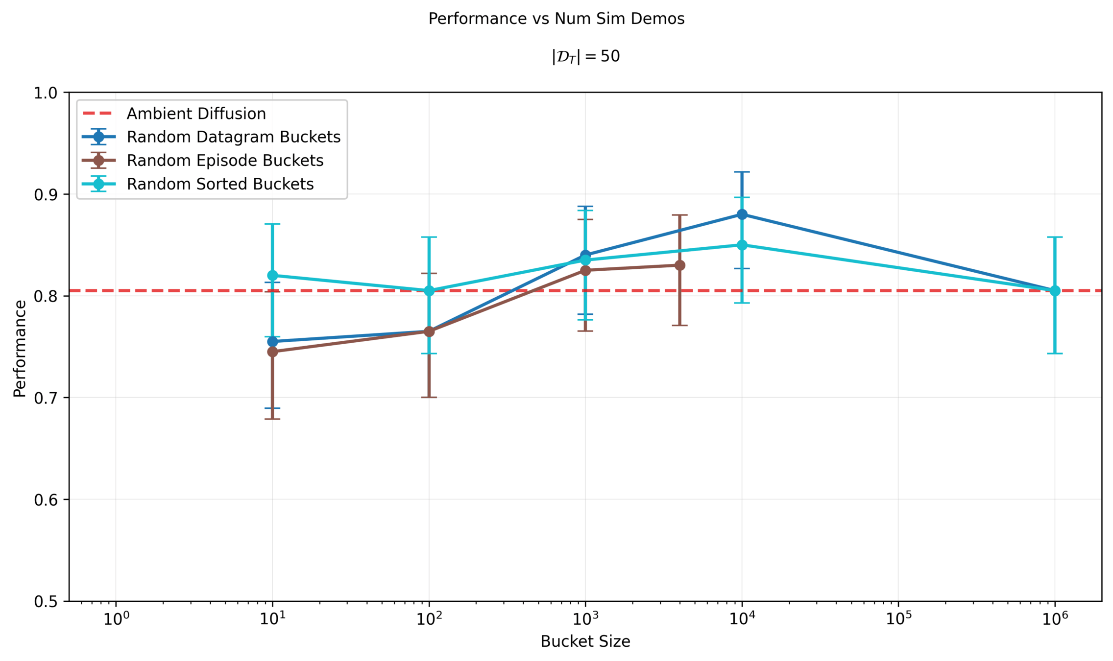
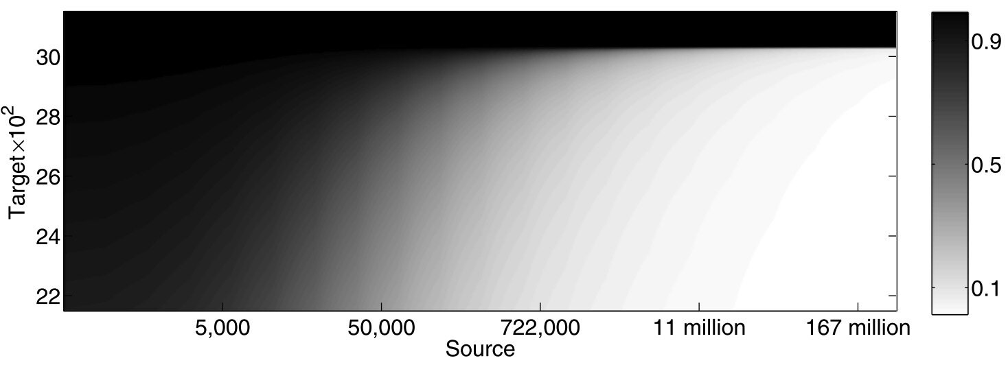
Problem 2: Ambient \(\to\) sim-only
\(|\mathcal{D}_S|=500\)
\(|\mathcal{D}_S|=4000\)
Sampling procedure:
- Sample \(\sigma\) ~ Unif([0,1])
- Sample (O, A, \(\sigma_{min}\)) ~ \(\mathcal{D}\) s.t. \(\sigma > \sigma_{min}\)
Denoising Loss vs Ambient Loss
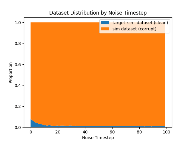
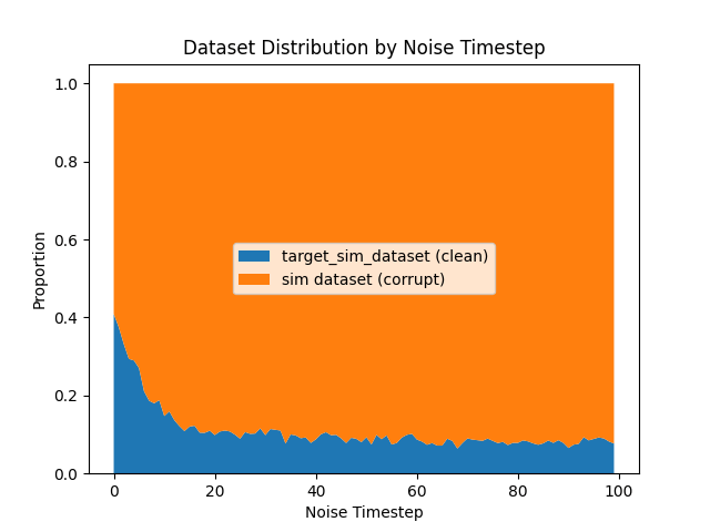
Solution: "Soft" Ambient Diffusion
"Doesn't make sense to use a hard threshold" - Pablo
(I am paraphrasing...)
Hard threshold!
\(\sigma=1\)
\(\sigma=0\)
\(\sigma=\sigma_{min}\)
Corrupt Data (\(\sigma_>\sigma_{min}\))
Clean Data (\(\sigma_{min}=0\))
Denoising Loss vs Ambient Loss
Different \(\alpha_\sigma\) per \(\sigma\in [0, 1]\)
"Doesn't make sense to use a hard threshold" - Pablo
(I am paraphrasing...)
\(\sigma=1\)
\(\sigma=0\)
Clean Data
Corrupt Data
Soft Ambient: ratio of clean to corrupt is a function of \(\alpha_\sigma\)
Ambient: ratio of clean to corrupt is a function of dataset size
Denoising Loss vs Ambient Loss
Why this should work
Optimal mixing ratio is a function of:
- Size of dataset 1
- Size of dataset 2
- \(D(p, q)\)
Ex. In binary classification and fixed \(D(p,q)\)...
Ben-David et. al, A theory of learning from different domains, 2009
Denoising Loss vs Ambient Loss
Why this should work
\(\sigma\)
\(D(p_\sigma, q_\sigma)\)
ratio for "bad" data
This idea is fits naturally in the noise as contraction interpretation.
Denoising Loss vs Ambient Loss
How to find \(\alpha^*(\sigma, n_1, n_2)\)
Have some ideas to find \(\alpha^*\) based on theoretical bounds...
... first try linear function just to get some signal.
\(\sigma=1\)
\(\sigma=0\)
Clean Data
Corrupt Data
Denoising Loss vs Ambient Loss
Will hopefully fix scaling issues?
Solution: bucketing
Ambient \(\to\) sim-only as \(|\mathcal{D}_S| \to \infty\)
... and sim-only is bad!
Classifier biases data distribution at different noise-levels
Problem 1
Problem 2
Solution: soft ambient
Part 5
Ambient Omni
Denoising Loss vs Ambient Loss
Locality
Ambient: "use low-quality data at high noise levels"
Ambient Omni: "use low-quality data at low and high noise levels"
- Leverages locality structure in many real world datasets
Denoising Loss vs Ambient Loss
Locality
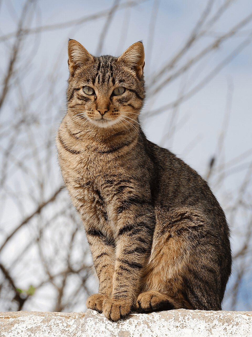
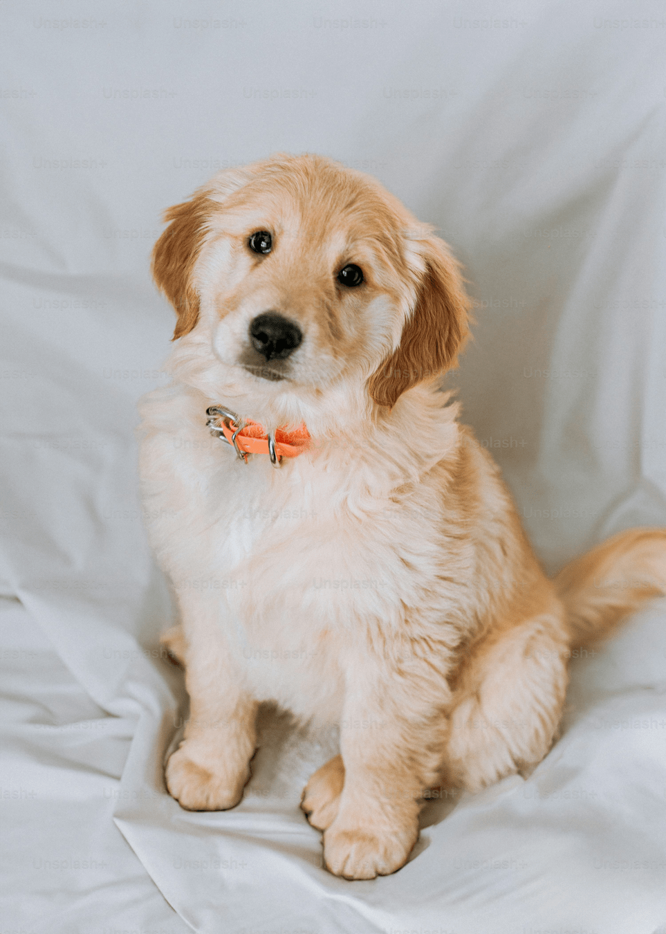
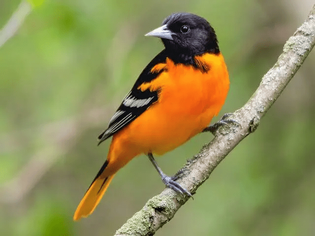
Which photo is the cat?
Denoising Loss vs Ambient Loss
Locality
Which photo is the cat?

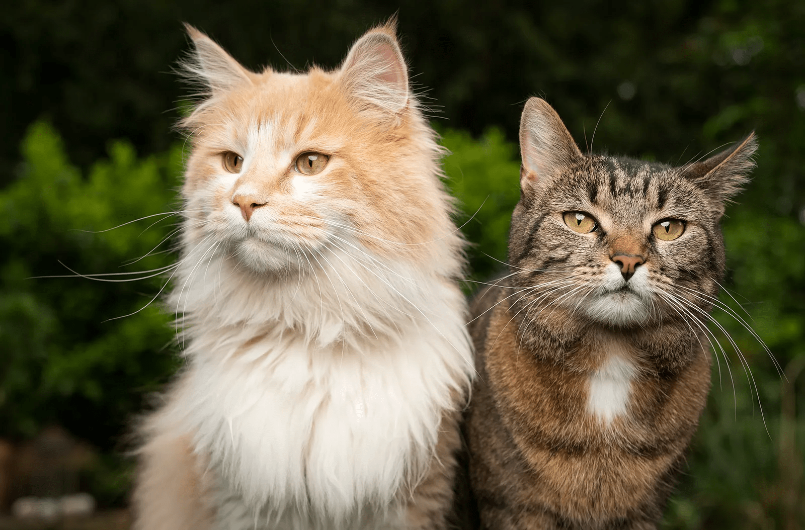
Which photo is the cat?
Locality
Locality
Which photo is the cat?
Locality
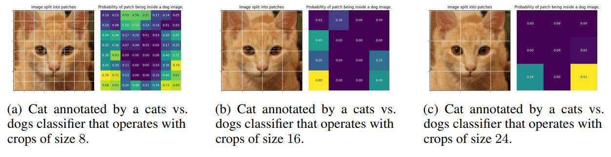
Loss vs Receptive Field
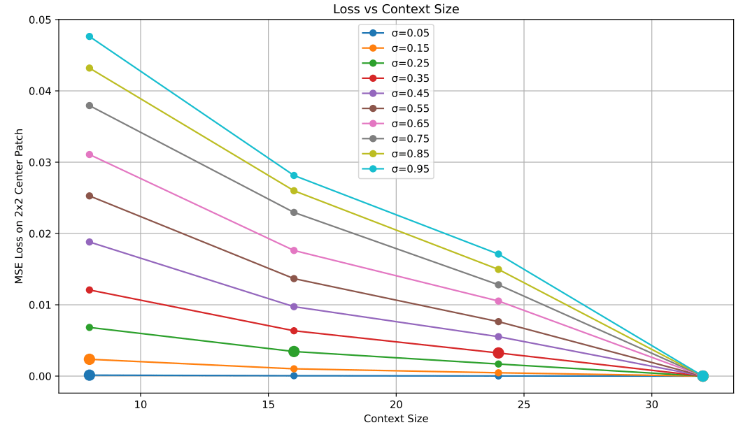
Receptive Field vs \(\sigma\)
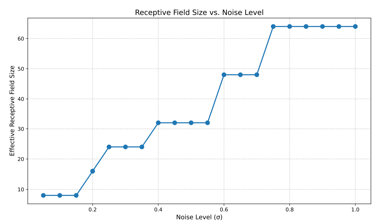
receptive field = \(f(\sigma)\)
Leveraging Locality
Intuition
- If \(p_\sigma \approx q_\sigma\) at receptive field \(f(\sigma)\), then \(q_\sigma\) can be used to learn \(p_\sigma\)
- The largest such \(\sigma\) is \(\sigma_{max}\)
receptive field = \(f(\sigma)\)
Ambient Omni
Repeat:
- Sample \(\sigma\) ~ Unif([0,1])
- Sample (O, A, \(\sigma_{min}, \sigma_{max}\)) ~ \(\mathcal{D}\) s.t. \(\sigma \in [0, \sigma_{max}) \cup (\sigma_{min}, 1]\)
- Optimize denoising loss or ambient loss
\(\sigma=0\)
\(\sigma>\sigma_{min}\)
\(\sigma_{min}\)
*\(\sigma_{min} = 0\) for all clean samples
\(\sigma=1\)
\(\sigma_{max}\)
\(\sigma>\sigma_{min}\)
\(\sigma_{max}\)
Implication for Robotics
\(\sigma=0\)
\(\sigma>\sigma_{min}\)
\(\sigma_{min}\)
\(\sigma=1\)
\(\sigma_{max}\)
\(\sigma>\sigma_{min}\)
\(\sigma_{max}\)
Task level
Motion level
- Data can be corrupt on the motion level and/or the task level
- Ambient handles motion level corruption
- Ambient Omni handles task level corruption as well
Example: Bin Sorting
Distribution shift: task level mismatch, motion level correctness
In-Distribution:
50 demos with correct sorting logic
Out-of-Distribution:
200 demos with arbitrary sorting
2x
2x
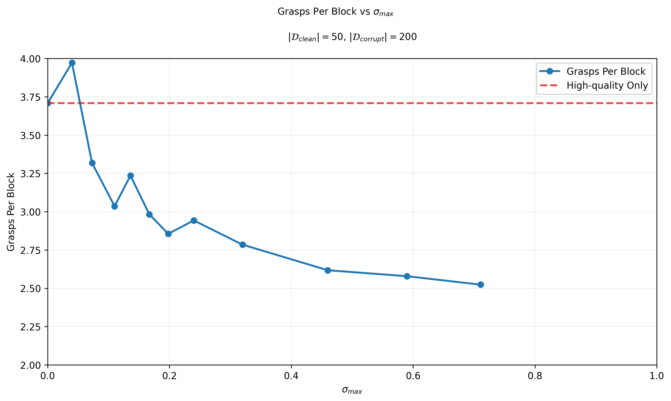
Example: Bin Sorting
Distribution shift: task level mismatch, motion level correctness
Contrived experiment... but it effectively illustrates the effect of \(\sigma_{max}\)
In-Distribution
Out-of-Distribution
2x
2x
Example: Bin Sorting
Contrived experiment... but it effectively illustrates the effect of \(\sigma_{max}\)
Repeat:
- Sample \(\sigma\) ~ Unif([0,1])
- Sample (O, A, \sigma_{max}\)) ~ \(\mathcal{D}\) s.t. \(\sigma \in [0, \sigma_{max})\)
- Optimize denoising loss
\(\sigma=0\)
\(\sigma=1\)
\(\sigma_{max}\)
\(\sigma>\sigma_{min}\)
\(\sigma_{max}\)
Results
Diffusion
Score
(Task + motion)
Correct logic
(Task level)
Cotrain
Completion
(Motion level)
Ambient-Omni
(\(\sigma_{max}=0.24\))
70.4%
48%
High...
55.2%
88%
Low...
94.0%
88%
97.5%
Results
Diffusion
Correct logic
(Task level)
Cotrain
Cotrain
(task conditioned)
Completion
(Motion level)
Ambient-Omni
(\(\sigma_{max}=0.24\))
70.4%
48%
High...
55.2%
88%
Low...
88.8%
86%
92.5%
94.0%
88%
97.5%
Score
(Task + motion)
Sweeping \(\sigma_{max}\): Task-Level Metrics
Motion Planning*
Task
Planning*
* not a binary distinction!!

Sweeping \(\sigma_{max}\): Motion Planning Metrics

Motion Planning
Task
Planning
* not a binary distinction!!
Sweeping \(\sigma_{max}\): Motion Planning Metrics
Motion Planning
Task
Planning
* not a binary distinction!!
Example: Bin Sorting
Distribution shift: task level mismatch, motion level correctness
In-Distribution
Out-of-Distribution
2x
2x
Open-X
Part 6
Concluding Thoughts
Project Roadmap
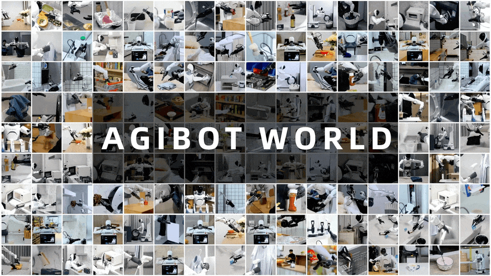
North Star Goal: Train with internet scale data (Open-X, AgiBot, etc)
So far: "Stepping stone" experiments
- Each experiment tests a specific part of the algorithm
Please suggest task ideas! Think big!
Revisting Distribution Shifts
- Sim2real gaps
- Noisy/low-quality teleop
- Task-level mismatch
- Changes in low-level controller
- Embodiment gap
- Camera models, poses, etc
- Different environment, objects, etc
robot teleop
simulation
Open-X
- Sim2real gaps
- Noisy/low-quality teleop
- Task-level mismatch
- Changes in low-level controller
- Embodiment gap
- Camera models, poses, etc
- Different environment, objects, etc
Revisting Distribution Shifts
- Sim2real gaps
- Noisy/low-quality teleop
- Task-level mismatch
- Changes in low-level controller
- Embodiment gap
- Camera models, poses, etc
- Different environment, objects, etc
- Observation space is a key part of robot data
- Currently not reasoning about corruption in the observations...
Revisting Distribution Shifts
Project Roadmap
- Sim2real gaps
- Noisy/low-quality teleop
- Task-level mismatch
- Changes in low-level controller
- Embodiment gap
- Camera models, poses, etc
- Different environment, objects, etc
Open-X
Project Roadmap
Open-X
Variant of Ambient Omni
Cool Task!!
(TBD)
Cool Demo!!
Thank you!! (please suggest tasks...)