Learning From Corrupt/Noisy Data
RLG Long Talk
May 2, 2025
Adam Wei
Agenda
- Motivation
- Ambient Diffusion
- Interpretation
- Experiments
... works in progress
Part 1
Motivation
Sources of Robot Data
Open-X
expert robot teleop
robot teleop
simulation

Goal: sample "high-quality" trajectories for your task
Train on entire spectrum to learn "high-level" reasoning, semantics, etc
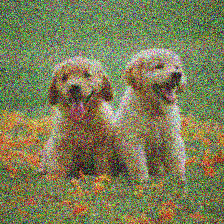
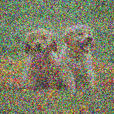
"corrupt"
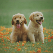
"clean"
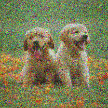
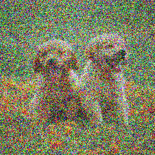
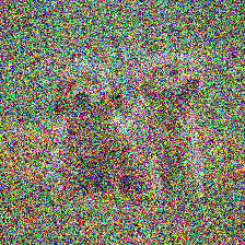
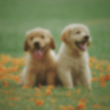
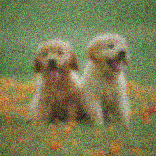
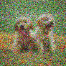
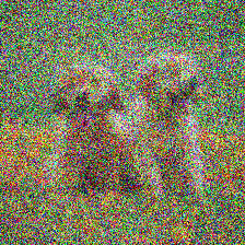
Corrupt Data
Corrupt Data
Clean Data
Computer Vision
Language


Poor writing, profanity, toxcity, grammar/spelling errors, etc


👀
Research Questions
- How can we learn from both clean and corrupt data?
- Can these algorithms be adapted for robotics?

Giannis Daras
Part 2a
Ambient Diffusion
Diffusion: Sample vs Epsilon Prediction
Epsilon prediction:
Sample prediction:
affine transform
Diffusion: VP vs VE
Variance preserving:
Variance exploding:
Variance exploding and sample-prediction simplify analysis
... analysis can be extended to DDPM
Ambient Diffusion
Assumptions
1. Each corrupt data point contains additive gaussian noise up to some noise level \(t_n\)
\(t=0\)
\(t=T\)
\(t=t_n\)


Corrupt data: \(X_{t_n} = X_0 + \sigma_{t_n} Z\)
Ambient Diffusion
Assumptions
1. Each corrupt data point contains additive gaussian noise up to some noise level \(t_n\)
2. \(t_n\) is known for each dataset or datapoint
\(t=0\)
\(t=T\)
\(t=t_n\)
Corrupt data: \(X_{t_n} = X_0 + \sigma_{t_n} Z\)
Naive Diffusion
\(t=0\)
\(t=T\)
\(t=t_n\)
noise
denoise
Forward Process
Backward Process
Can we do better?
\(t=0\)
\(t=T\)
\(t=t_n\)
noise
denoise
Forward Process
Backward Process
Can we do better?
\(t=0\)
\(t=T\)
\(t=t_n\)
noise
denoise
How can we learn \(h_\theta^*(x_t, t) = \mathbb E[X_0 | X_t = x_t]\) using noisy samples \(X_{t_n}\)?
Ambient Diffusion
Ambient Loss
Note that this loss does not require access to \(x_0\)
How can we learn \(h_\theta^*(x_t, t) = \mathbb E[X_0 | X_t = x_t]\) using noisy samples \(X_{t_n}\)?
Diffusion Loss
No access to \(x_0\)
Ambient Diffusion
We can learn \(\mathbb E[X_0 | X_t=x_t]\) using only corrupted data!
Remarks
- From any given \(x_{t_n}\), you cannot recover \(x_0\)
- Given \(p_{X_{t_n}}\), you can compute \(p_{X_0}\)
- "No free lunch": learning \(p_{X_0}\) from \(X_{t_n}\) requires more samples than learning from clean data \(X_0\)
Proof: "Double Tweedies"
\(X_{t} = X_0 + \sigma_{t}Z\)
\(X_{t} = X_{t_n} + \sqrt{\sigma_t^2 - \sigma_{t_n}^2}Z\)
\(\nabla \mathrm{log} p_t(x_t) = \frac{\mathbb E[X_0|X_t=x_t]-x_t}{\sigma_t^2}\)
\(\nabla \mathrm{log} p_t(x_t) = \frac{\mathbb E[X_{t_n}|X_t=x_t]-x_t}{\sigma_t^2-\sigma_{t_n}^2}\)
(Tweedies)
(Tweedies)
Proof: "Double Tweedies"
\(g_\theta(x_t,t) := \frac{\sigma_t^2 - \sigma_{t_n}^2}{\sigma_t^2} h_\theta(x_t,t) + \frac{\sigma_{t_n}^2}{\sigma_t^2}x_t\).
Ambient loss:
Proof: "Double Tweedies"
\(\frac{\sigma_t^2 - \sigma_{t_n}^2}{\sigma_t^2} h_\theta^*(x_t,t) + \frac{\sigma_{t_n}^2}{\sigma_t^2}x_t = \mathbb E [X_{t_n} | X_t = x_t]\)
(from double Tweedies)
\(\implies\)
\(\implies\)
(definition of \(g_\theta\))
Training Algorithm
For each data point:
Clean data: \(t\in (0, T]\)
\(x_t = x_0 + \sigma_t z\)
\(\mathbb E[\lVert h_\theta(x_t, t) - x_0 \rVert_2^2]\)
Forward process:
Backprop:
Corrupt data
\(t\in (t_n, T]\)
\(x_t = x_{t_n} + \sqrt{\sigma_t^2-\sigma_{t_n}^2} z_2\)
\(\mathbb E[\lVert \frac{\sigma_t^2 - \sigma_{t_n}^2}{\sigma_t^2} h_\theta(x_t,t) + \frac{\sigma_{t_n}^2}{\sigma_t^2} - x_{t_n} \rVert_2^2]\)
Ambient Diffusion
\(t=0\)
\(t=T\)
\(t=t_n\)
\(\mathbb E[\lVert h_\theta(x_t, t) - x_0 \rVert_2^2]\)
\(\mathbb E[\lVert \frac{\sigma_t^2 - \sigma_{t_n}^2}{\sigma_t^2} h_\theta(x_t,t) + \frac{\sigma_{t_n}^2}{\sigma_t^2}x_t - x_{t_n} \rVert_2^2]\)
Use clean data to learn denoisers for \(t\in(0,T]\)
Use corrupt data to learn denoisers for \(t\in(t_n,T]\)
Part 2b
Ambient Diffusion w/ Contraction
Protein Folding Case Study
Case Study: Protein Folding
Assumptions
1. Each corrupt data point contains additive gaussian noise up to some noise level \(t_n\)
2. \(t_n\) is known for each dataset or datapoint
\(t=0\)
\(t=T\)
\(t=t_n\)
Corrupt data: \(X_{t_n} = X_0 + \sigma_{t_n} Z\)
Case Study: Protein Folding
Corrupt Data
Clean Data


+ 5 years
=
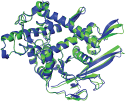
~100,000 solved protein structures
200M+ protein structures
Case Study: Protein Folding
Corrupt Data
Clean Data
\(X_0^{corrupt} \neq X_0^{clean} + \sigma_{t_n} Z\)
Breaks both assumptions:
- Corruption is not additive Gaussian noise
- Don't know \(t_n\) for each AlphaFold protein
\(X_0^{clean}\)
\(X_0^{corrupt}\)
Corrupt Data
Clean Data
Corrupt Data + Noise

For sufficiently high \(t_n\): \(X_{t_n}^{corrupt} = X_0^{corrupt} + \sigma_{t_n} Z \approx X_0^{clean} + \sigma_{t_n} Z\)
\(X_{t_n}^{corrupt} = X_0^{corrupt} + \sigma_{t_n} Z\)
Key idea: Corrupt data further with Gaussian noise
Assumption 1: Contraction


\(X_0^{clean}\)
\(X_0^{corrupt}\)
\(X_{t_n}^{corrupt}\)
Key idea: Corrupt data further with Gaussian noise
For sufficiently high \(t_n\): \(X_{t_n}^{corrupt} = X_0^{corrupt} + \sigma_{t_n} Z \approx X_0^{clean} + \sigma_{t_n} Z\)

\(x_0^{clean}\)
\(x_0^{corrupt}\)
\(t=0\)
\(t=T\)
\(t=t_n\)
Assumption 1: Contraction
For sufficiently high \(t_n\): \(X_{t_n}^{corrupt} \approx X_0^{clean} + \sigma_{t_n} Z\)
\(P_{Y|X}\)
\(Y = X + \sigma_{t_n} Z\)
\(P_{X_0}^{clean}\)
\(Q_{X_0}^{corrupt}\)
\(P_{X_{t_n}}^{clean}\)
\(Q_{X_{t_n}}^{corrupt}\)
Assumption 1: Contraction
\(\implies\) Adding noise makes the corruption appear Gaussian (Assumption 1)
- Clean and corrupt data share coarse structure
- Adding noise masks high-frequency differences, preserves low frequency similarities
\(x_0^{clean}\)
\(x_0^{corrupt}\)
\(t=0\)
\(t=T\)
\(t=t_n\)
Assumption 1: Intuition
Assumption 2: Finding \(t_n\)
1. Train a "clean" vs "corrupt" classifier for all \(t \in [0, T]\)
2. For each corrupt data point, increase noise until the classification accuracy drops. This is \(t_n\).
\(x_0^{clean}\)
\(x_0^{corrupt}\)
\(t=0\)
\(t=T\)
\(t=t_n\)
Training Algorithm
For each data point:
Clean data
\(x_t = x_0 + \sigma_t z\)
\(\mathbb E[\lVert h_\theta(x_t, t) - x_0 \rVert_2^2]\)
Forward process:
Backprop:
Corrupt data
\(x_t = x_{t_n} + \sqrt{\sigma_t^2-\sigma_{t_n}^2} z_2\)
\(x_{t_n} = x_0 + \sigma_{t_n} z_1\)
Contract data:
\(\mathbb E[\lVert \frac{\sigma_t^2 - \sigma_{t_n}^2}{\sigma_t^2} h_\theta(x_t,t) + \frac{\sigma_{t_n}^2}{\sigma_t^2} - x_{t_n} \rVert_2^2]\)
Part 3
Interpretations
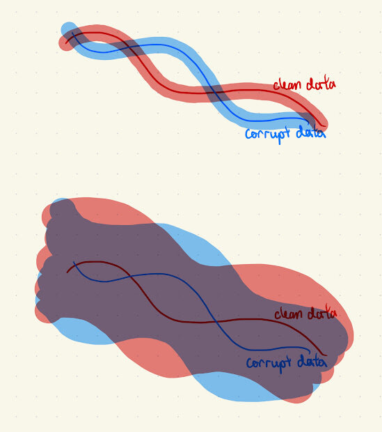
Frequency Domain Interpretation
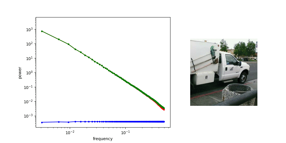
Diffusion is AR sampling in the frequency domain
Frequency Domain Interpretation*
\(t=0\)
\(t=T\)
\(t=t_n\)
Low Frequency
High Frequency
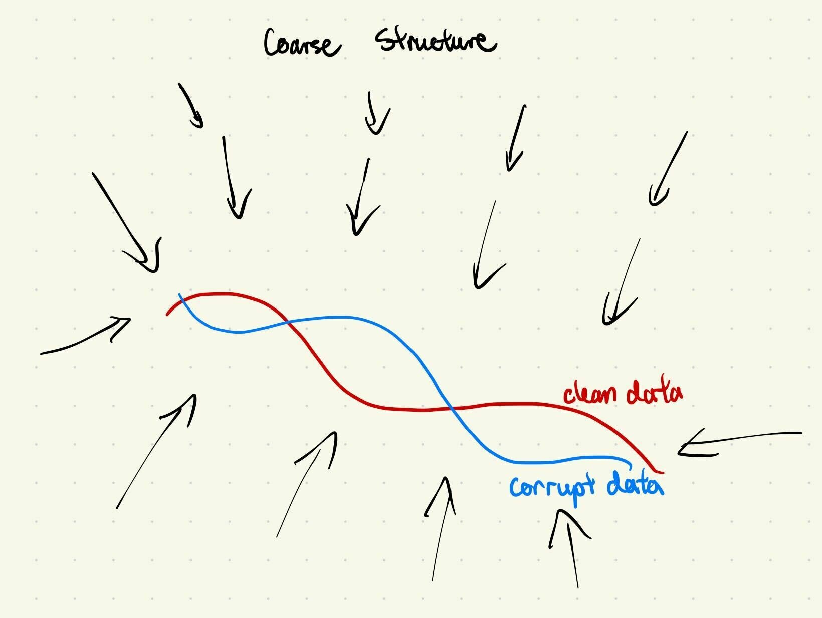
Coarse Structure
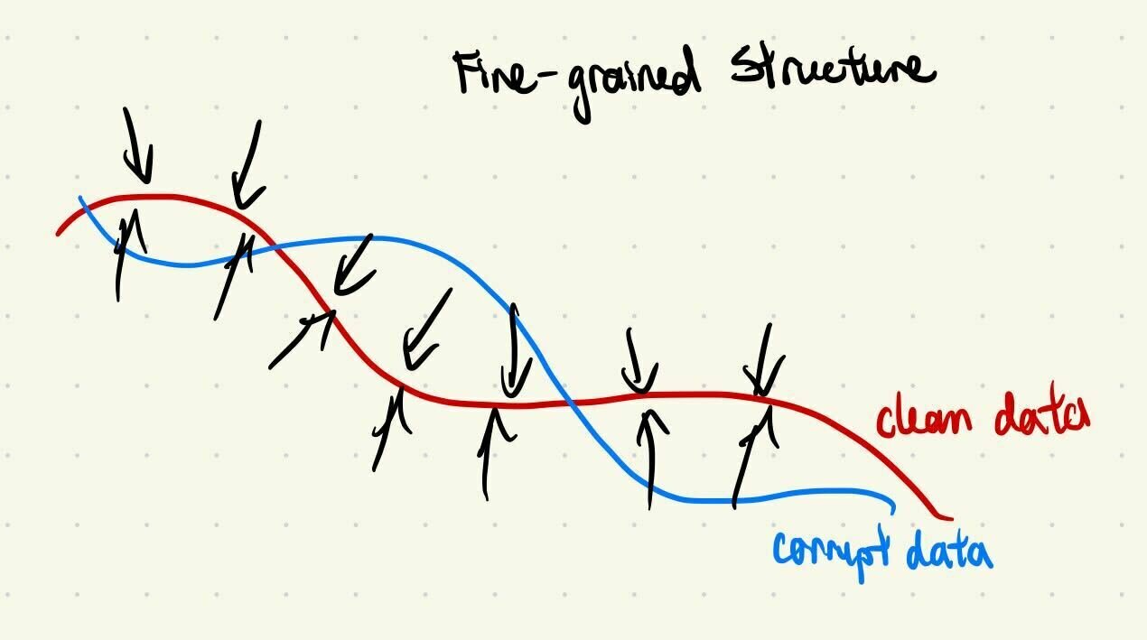
Fine-grained Details
* assuming power spectral density of data is decreasing
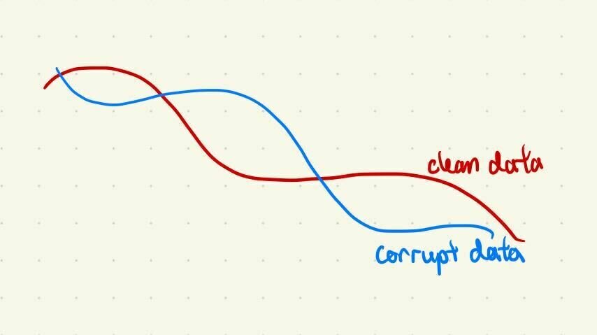
Frequency Domain Interpretation
\(t=0\)
\(t=T\)
\(t=t_n\)
\(\mathbb E[\lVert h_\theta(x_t, t) - x_0 \rVert_2^2]\)
\(\mathbb E[\lVert \frac{\sigma_t^2 - \sigma_{t_n}^2}{\sigma_t^2} h_\theta(x_t,t) + \frac{\sigma_{t_n}^2}{\sigma_t^2}x_t - x_{t_n} \rVert_2^2]\)
Low Freq
High Freq
Clean & corrupt data share the same "coarse structure"
Learn coarse structure from all data
Learn fine-grained details from clean data only
i.e. same low frequency features
Clean Data
Corrupt Data
Robotics Hypothesis
Hypothesis: Robot data shares low-frequency features, but differ in high frequency features
Clean & corrupt data share the same "coarse structure"
i.e. same low frequency features
Low Frequency
- Move left or right
- Semantics & language
- High-level decision making
Learn with Open-X, AgiBot, sim, clean data, etc
High Frequency
- Environment physics/controls
- Task-specific movements
- Specific embodiment
Learn from clean task-specific data
"Manifold" Interpretation
Diffusion is Euclidean projection onto the data manifold
Assumption: The clean and corrupt data manifolds lie in a similar part of space, but differ in shape
"Manifold" Interpretation
Diffusion is Euclidean projection onto the data manifold
Large \(\sigma_t\)
Both clean and corrupt data project to close to the clean data manifold
"Manifold" Interpretation
Diffusion is Euclidean projection onto the data manifold
Small \(\sigma_t\)
Use clean data to project onto the clean data manifold
Part 4
Robotics??
Robotics
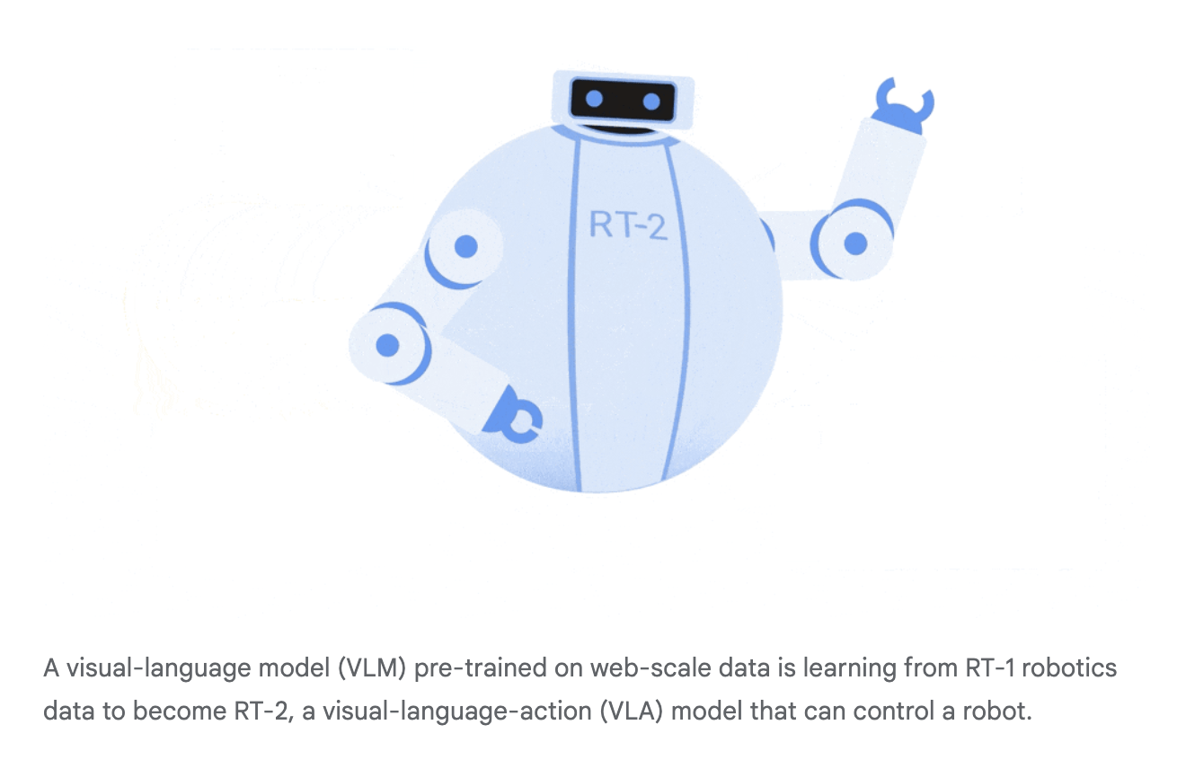
Open-X
expert robot teleop
robot teleop
simulation
"corrupt"
"clean"
Start by exploring ideas inspired by Ambient Diffusion on sim-and-real cotraining
Robotics: Sim-and-Sim Cotraining
Corrupt Data (Sim): \(\mathcal D_S\)
Clean Data (Real): \(\mathcal D_T\)
Replayed GCS plans in Drake
Sources of corruption: (non-Gaussian...)
- Physics gap
- Visual gap
- Action gap
Teleoperated demos in a target-sim environment
... sorry no video :(
Robotics Idea 1: Modified Diffusion
- Assume all simulated data points in \(\mathcal D_S\) are corrupted with some fixed level \(t_n\)
- For \(t > t_n\): train denoisers with clean and corrupt data
- For \(t \leq t_n\): train denoisers with only clean data
- Use regular DDPM loss (i.e. not ambient loss)
- Since the sim_data \(\neq\) real_data + noise
Training:
Robotics Idea 1: Modified Diffusion
\(t=0\)
\(t=T\)
\(t=t_n\)
\(\mathbb E[\lVert h_\theta(x_t, t) - x_0^{clean} \rVert_2^2]\)
\(\mathbb E[\lVert h_\theta(x_t, t) - x_0^{corrupt} \rVert_2^2]\)
Low Freq
High Freq
Learn with all data
Learn with clean data
Clean Data
Corrupt Data
Intuition: mask out high-frequency components of "corrupt" data
Robotics Idea 1
Robotics Idea 2: Ambient w/o Contraction
\(t=0\)
\(t=T\)
\(t=t_n\)
\(\mathbb E[\lVert h_\theta(x_t, t) - x_0^{clean} \rVert_2^2]\)
Low Freq
High Freq
Learn with all data
Learn with clean data
Clean Data
Corrupt Data
Assume \(X_0^{corrupt} = X_{t_n}^{clean} = X_0^{clean} + \sigma_{t_n} Z\)
(NOT TRUE)
\(\mathbb E[\lVert \frac{\sigma_t^2 - \sigma_{t_n}^2}{\sigma_t^2} h_\theta(x_t,t) + \frac{\sigma_{t_n}^2}{\sigma_t^2}x_t - x_0^{corrupt} \rVert_2^2]\)
Robotics Idea 1
Results: Idea 1
- 50 clean (real) demos
- 2000 corrupt (sim) demos
- 200 trials each
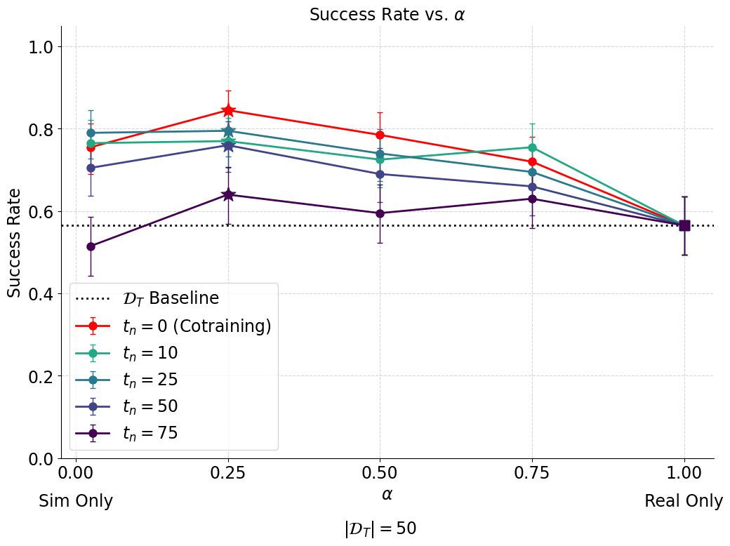
Results are currently worse than the cotraining baseline :(
Robotics Idea 1
Discussion: Idea 1
- Ambient diffusion loss rescaling
- Real and sim data are too similar at all noise levels
- \(\implies\) no incentive to mask out high-frequency components of "corrupt" data
- Will potentially find more success using Open-X, AgiBot, etc
- Image conditioning is sufficient to disambiguate sampling from clean (real) vs corrupt (sim)
\(\mathbb E[\lVert \frac{\sigma_t^2 - \sigma_{t_n}^2}{\sigma_t^2} h_\theta(x_t,t) + \frac{\sigma_{t_n}^2}{\sigma_t^2}x_t - x_{t_n} \rVert_2^2]\)
\(\mathbb E[\lVert h_\theta(x_t,t) + \frac{\sigma_{t_n}^2}{\sigma_t^2-\sigma_{t_n}^2}x_t - \frac{\sigma_t^2}{\sigma_t^2 - \sigma_{t_n}^2}x_{t_n} \rVert_2^2]\)
Ambient Loss
"Rescaled" Ambient Loss
... blows up for small \(\sigma_t\)
Robotics Idea 1
Discussion: Idea 1
- Ambient diffusion loss rescaling
- Real and sim data are too similar at all noise levels
- \(\implies\) no incentive to mask out high-frequency components of "corrupt" data
- Will potentially find more success using Open-X, AgiBot, etc
- Image conditioning is sufficient to disambiguate sampling from clean (real) vs corrupt (sim)
- Hyperparameter sweep
Robotics Idea 1
Results: Idea 2
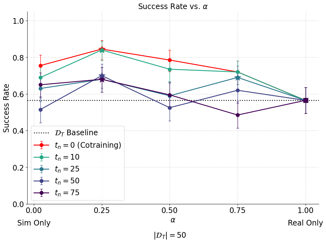
Worse than idea 1, but this was expected
Assume \(X_0^{corrupt} = X_{t_n}^{clean} = X_0^{clean} + \sigma_{t_n} Z\)
(NOT TRUE)
Robotics Idea 1
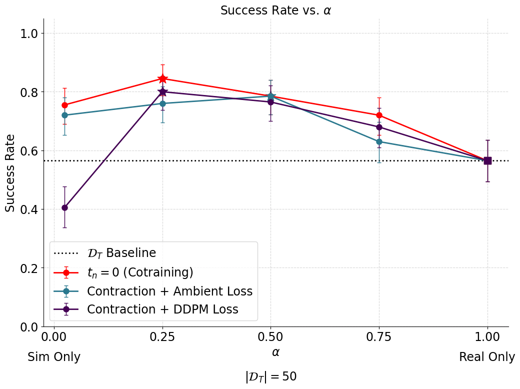
Idea 3: Ambient w/ Contraction
1. Train a binary classifier to distinguish sim vs real actions
2. Use the classifier to find \(t_n\) for all sim actions in \(\mathcal D_S\)
3. Noise all sim actions to \(t_n\):
\(X_{t_n}^{corrupt} = X_0^{corrupt} + \sigma_{t_n} Z\)
\(\approx X_0^{clean} + \sigma_{t_n} Z\)
4. Train with ambient diffusion and \(t_n\) per datapoint
*same algorithm as SOTA protein folding
Robotics Idea 1
Idea 3: Ambient w/ Contraction
1. Train a binary classifier to distinguish sim vs real actions
2. Use the classifier to find \(t_n\) for all sim actions in \(\mathcal D_S\)
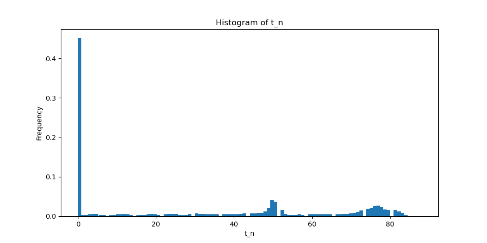
\(t_n\) = 0 for 40%+ of action sequences... \(\implies\) sim data is barely corrupt
Robotics Idea 1
Idea 3: Ambient w/ Contraction
Robotics Idea 1
Idea 4: ... but first recall idea 1
\(t=0\)
\(t=T\)
\(t=t_n\)
\(\mathbb E[\lVert h_\theta(x_t, t) - x_0^{clean} \rVert_2^2]\)
\(\mathbb E[\lVert h_\theta(x_t, t) - x_0^{corrupt} \rVert_2^2]\)
Low Freq
High Freq
Learn with all data
Learn with clean data
Clean Data
Corrupt Data
Robotics Idea 1
Idea 4: Different \(\alpha_t\) per \(t\in (0, T]\)
\(t=0\)
\(t=T\)
Low Freq
High Freq
Clean Data
Corrupt Data
- Train with different data mixtures \(\alpha_t\) at different noise levels
\(\mathbb E[\lVert h_\theta(x_t, t) - x_0^{clean} \rVert_2^2]\)
\(\mathbb E[\lVert h_\theta(x_t, t) - x_0^{corrupt} \rVert_2^2]\)
\(\alpha_T\)
\(\alpha_0\)
Robotics Idea 1
Idea 4: Different \(\alpha_t\) per \(t\in (0, T]\)
\(D(\red{p^{clean}_{\sigma_t}}||\blue{p^{corrupt}_{\sigma_t}})\) is large
\(\implies\) sample more clean data
Low noise levels
(small \(\sigma_t\))
High noise levels
(large \(\sigma_t\))
\(D(\red{p^{clean}_{\sigma_t}}||\blue{p^{corrupt}_{\sigma_t}})\) is small
\(\implies\) sample more corrupt data
Robotics Idea 1
Next Directions
- Try to improve results for all 4 ideas on planar pushing
- Try ambient diffusion related ideas for cotraining from Open-X or AgiBot
Robotics Idea 1
Thoughts
Motivating ideas for ambient diffusion
- Noise as partial masking (mask out high frequency corruption)
- Clean and corrupt distributions are more similar at high noise levels
Motivating ideas could be useful for robotics, but the exact Ambient Diffusion algorithm might not??