Unifying Perspectives on Diffusion
RLG Short Talk
May 3, 2024
Adam Wei
Interpretations of Diffusion
Goal: Show how the different interpretations of diffusion are connected.
Diffusion
Sohl-Dickstein et al
DDPM
Ho et al
SMLD
Song et al
SDE
Song et al
Projection
Permenter et al
2015
2019
2021
2023
Denoising
Score-based
Optimization
2020
What this presentation is not...
- Not a deep dive into the papers
- Not a rigorous mathematical presentation
- Not about how to train diffusion policies or score-matching
Goal: Show how the different interpretations of diffusion are connected.
SDE Interpretation
Summary
2. Score-based and denoiser approaches are discrete instantiations of the SDE approach
1. Both SMLD and DDPM learn the score function of the noisy distributions.
Interpretations of Diffusion Policy
Diffusion
Sohl-Dickstein et al
DDPM
Ho et al
SMLD
Song et al
SDE
Song et al
Projection
Permenter et al
2015
2019
2021
2023
Denoising
Score-based
Optimization
2020
Goal: Show how the different interpretations of diffusion are connected.
SMLD: Langevin Dynamics (1/5)
Intuition: On each step..
Key Takeaway: under regularity conditions
- Move in a direction that increases log probability
- Add Gaussian noise (prevent collapse onto peaks of p)
"Score Function"
Goal: Sample from some distribution p
SMLD: Langevin Dynamics (2/5)
"Gradient ascent with Gaussian noise"

SMLD: Algorithm (3/5)
1. Construct sequence of noised distributions:
2. Learn
3. Sample from annealed Langevin Dynamics
SMLD: Algorithm (4/5)
Advantages
- Faster convergence
- Better learned scores
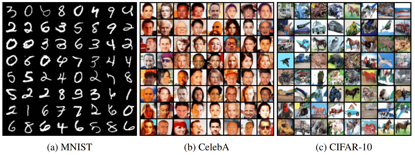
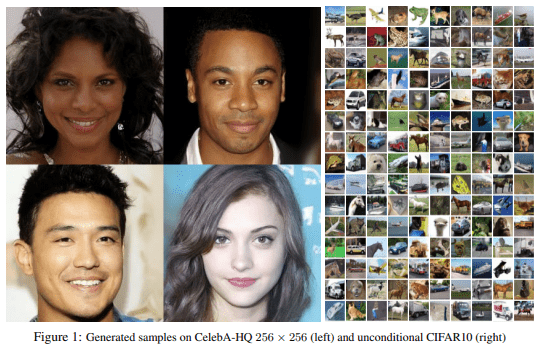
SMLD: Results (5/5)
SMLD: Connection to control... (Bonus)
1. Design a trajectory in distribution space
2. Use Langevin Dynamics to track this trajectory
TODO: DRAW IMAGE
Interpretations of Diffusion Policy
Diffusion
Sohl-Dickstein et al
DDPM
Ho et al
SMLD
Song et al
SDE
Song et al
Projection
Permenter et al
2015
2019
2021
2023
Denoising
Score-based
Optimization
2020
Goal: Show how the different interpretations of diffusion are connected.
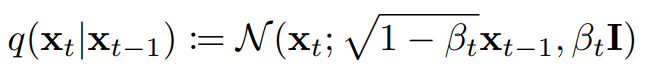
DDPM: Overview (1/6)
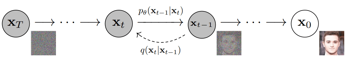
Forward Process: Noise the data
Backward Process: Denoising
DDPM: Results (2/6)
DDPM vs SMLD (3/6)
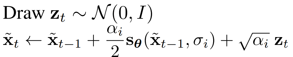
SMLD Sampling:
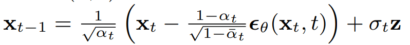
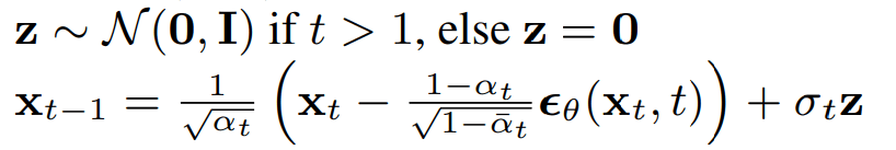
DDPM Sampling:
Screenshots from the papers. Notation is not same!!
DDPM vs SMLD (4/6)
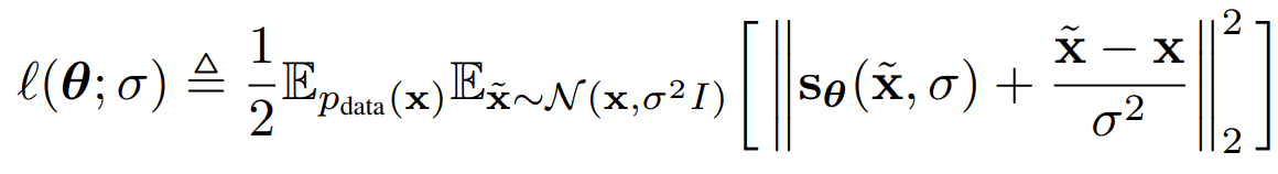
SMLD Loss
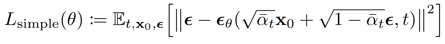
DDPM Loss
Screenshots of original loss functions. Notation is not same!!
DDPM vs SMLD (5/6)
SMLD Loss*:
DDPM Loss*:
*Rewritten loss functions with severe abuse of notation to highlight similarities.
DDPM: Connection to Score-Matching (6/6)
Key Takeaway
SDE Interpretation
Interpretations of Diffusion Policy
Diffusion
Sohl-Dickstein et al
DDPM
Ho et al
SMLD
Song et al
SDE
Song et al
Projection
Permenter et al
2015
2019
2021
2023
Denoising
Score-based
Optimization
2020
Goal: Show how the different interpretations of diffusion are connected.
SDE Interpretation
SDE: Overview (1/8)
SMLD/DDPM: Noise and denoise in discrete steps.
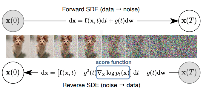
SDE: Noise and denoise according to continuous SDEs
SDE Interpretation
SDE: Overview (2/8)
Key Takeaway: SMLD and DDPM are discrete instances of the SDE interpretation!
SDE Interpretation
SDE: Ito-SDE (3/8)
[1] Bernt Øksendal, 2003 [2] Brian D O Anderson, 1982
1. If f and g are Lipschitz, the Ito-SDE has a unique solution [1].
2. The reverse-time SDE is [2]:
"Ito-SDE"
SDE Interpretation
SDE: Algorithm (4/8)
1. Define f and g s.t. X(0) ~ p transforms into a tractable distribution, X(T)
2. Learn
3. To sample:
- Draw sample x(T)
- Reverse the SDE until t=0
SMLD/DDPM
SDE Interpretation
SDE: SMLD (5/8)
Forward (N-steps):
SDE Interpretation
SDE: SMLD (6/8)
SDE Interpretation
SDE: DDPM (7/8)
Forward (N-steps):
SDE Interpretation
SDE: Summary (8/8)
SDE Interpretation:
Forward:
Reverse:
SMLD
DDPM
SDE Interpretation
Summary
2. Score-based and denoiser approaches are discrete instantiations of the SDE approach
1. Both SMLD and DDPM learn the score function of the noisy distributions.
SDE Interpretation
Resources
Papers: Sohl-Dickstein, SMLD, DDPM, SDE, Permenter, Understanding Diffusion Models
Blogs: Lillian Weng, Yang Song, Peter E. Holderrieth
Tutorials: Yang Song, "What are Diffusion Models"
Diffusion in Robotics: https://github.com/mbreuss/diffusion-literature-for-robotics