A Quick Overview of POMDP Solution Methods

Markov Model
- \(\mathcal{S}\) - State space
- \(T:\mathcal{S}\times\mathcal{S} \to \mathbb{R}\) - Transition probability distributions
Markov Decision Process (MDP)
- \(\mathcal{S}\) - State space
- \(T:\mathcal{S}\times \mathcal{A} \times\mathcal{S} \to \mathbb{R}\) - Transition probability distribution
- \(\mathcal{A}\) - Action space
- \(R:\mathcal{S}\times \mathcal{A} \to \mathbb{R}\) - Reward

Partially Observable Markov Decision Process (POMDP)

- \(\mathcal{S}\) - State space
- \(T:\mathcal{S}\times \mathcal{A} \times\mathcal{S} \to \mathbb{R}\) - Transition probability distribution
- \(\mathcal{A}\) - Action space
- \(R:\mathcal{S}\times \mathcal{A} \to \mathbb{R}\) - Reward
- \(\mathcal{O}\) - Observation space
- \(Z:\mathcal{S} \times \mathcal{A}\times \mathcal{S} \times \mathcal{O} \to \mathbb{R}\) - Observation probability distribution
Objective Function
$$\underset{\pi}{\mathop{\text{maximize}}} \, E\left[\sum_{t=0}^{\infty} \gamma^t R(s_t, \pi(\cdot)) \right]$$
\(Q^\pi(s, a)\) = Expected sum of future rewards
- Starting at \((s,a)\)
- Following \(\pi\) thereafter
POMDP Sense-Plan-Act Loop
Environment
Belief Updater
Planner/Policy
\(o\)
\(b\)
\(a\)
Aggressive: 63%
Normal: 34%
Timid: 3%
\(x, y, v\)
Turn Left
C. H. Papadimitriou and J. N. Tsitsiklis, “The complexity of Markov decision processes,” Mathematics of Operations Research, vol. 12, no. 3, pp. 441–450, 1987
Computational Complexity

POMDPs
(PSPACE Complete)
Model Approximations
Try to solve something other than a POMDP
Numerical Approximations
Converge to the optimal POMDP solution
Model Approximations
- QMDP
- Fast Informed Bound
- Hindsight Optimization
- Ignore Observations
- Most Likely Observation
Numerical Approximations
Converge to the optimal POMDP solution
QMDP
POMDP:
QMDP:
\[\pi_{Q_\text{MDP}}(b) = \underset{a\in\mathcal{A}}{\text{argmax}} \underset{s\sim b}{E}\left[Q_\text{MDP}(s,a)\right]\]
where \(Q_\text{MDP}\) are the optimal \(Q\) values for the fully observable MDP.
$$\pi^* = \underset{\pi}{\mathop{\text{argmax}}} \, E\left[\sum_{t=0}^{\infty} \gamma^t R(s_t, \pi(b_t)) \right]$$
QMDP

INDUSTRIAL GRADE
QMDP


ACAS X
[Kochenderfer, 2011]

[Sunberg, 2018]
Ours
Suboptimal
State of the Art
Discretized


Offline
- Find a solution for all possible beliefs offline, then use look-up table online
- Typically use point-based value iteration with \(\alpha\)-vectors
Online
- Find solution for current belief online
- Typically use heuristic search or Monte Carlo Tree Search
Numerical POMDP Solvers
| (S,A,O) | Offline | Online |
|---|---|---|
| (D,D,D) | All PBVI Variants SARSOP |
AEMS |
| (C,D,D) | POMCP DESPOT |
|
| (C,D,C) | MCVI | POMCPOW DESPOT-alpha |
| (C,C,C) |
(All solvers can also handle the cells above)
Special Cases/RL Only
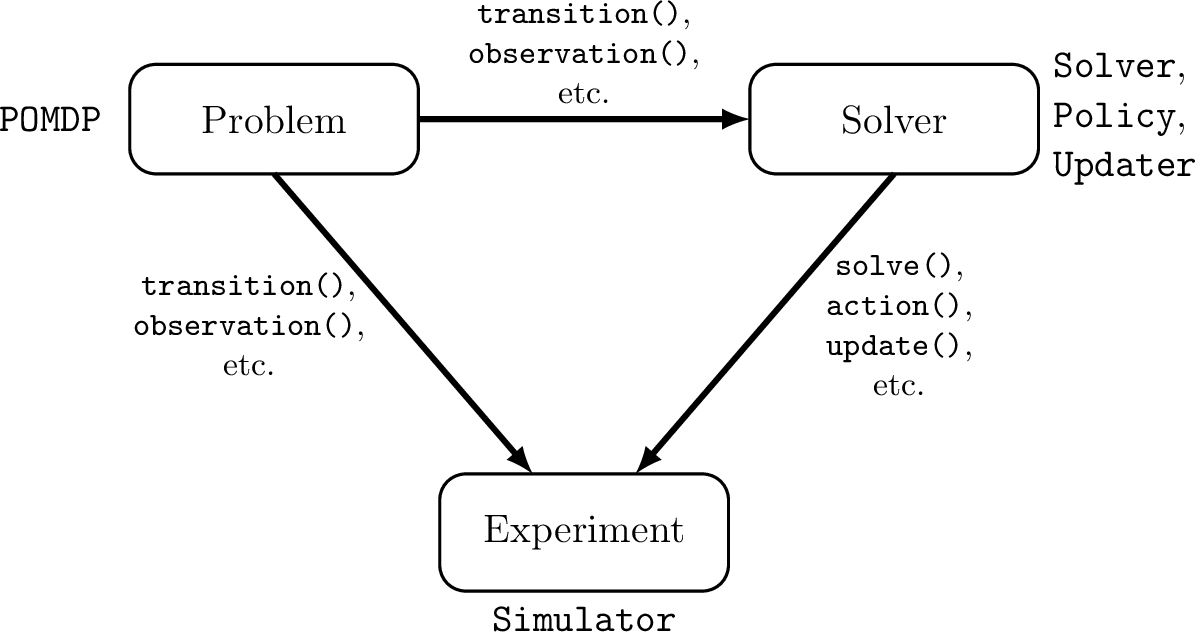
POMDPs.jl - An interface for defining and solving MDPs and POMDPs in Julia
PBVI/SARSOP
Efficiency comes from judiciously choosing beliefs for backup

- A POMDP is an MDP on the Belief Space but belief updates are expensive
- POMCP* uses simulations of histories instead of full belief updates
- Each belief is implicitly represented by a collection of unweighted particles


[Ross, 2008] [Silver, 2010]
*(Partially Observable Monte Carlo Planning)
Types of Uncertainty
ALEATORY
MODEL (Epistemic, Static)
STATE (Epistemic, Dynamic)


\begin{aligned}
& \mathcal{S} = \mathbb{Z} \quad \quad \quad ~~ \mathcal{O} = \mathbb{R} \\
& s' = s+a \quad \quad o \sim \mathcal{N}(s, s-10) \\
& \mathcal{A} = \{-10, -1, 0, 1, 10\} \\
& R(s, a) = \begin{cases}
100 & \text{ if } a = 0, s = 0 \\
-100 & \text{ if } a = 0, s \neq 0 \\
-1 & \text{ otherwise}
\end{cases} & \\
\end{aligned}

State
Timestep
Accurate Observations
Goal: \(a=0\) at \(s=0\)
Optimal Policy
Localize
\(a=0\)
POMDP Example: Light-Dark
POMDP Solution
QMDP


Same as full observability on the next step
Environment
Belief Updater
Policy
\(a\)
\(b = \mathcal{N}(\hat{s}, \Sigma)\)
True State
\(s \in \mathbb{R}^n\)
Observation \(o \sim \mathcal{N}(C s, V)\)
LQG Problem (a simple POMDP)
\(s_{t+1} \sim \mathcal{N}(A s_t + B a_t, W)\)
\(\pi(b) = K \hat{s}\)
Kalman Filter
\(R(s, a) = - s^T Q s - a^T R a\)
QMDP
POMDP:
QMDP:
\[\pi_{Q_\text{MDP}}(b) = \underset{a\in\mathcal{A}}{\text{argmax}} \underset{s\sim b}{E}\left[Q_\text{MDP}(s,a)\right]\]
where \(Q_\text{MDP}\) are the optimal \(Q\) values for the fully observable MDP. \(O(T |S|^2|A|)\)
$$\pi^* = \underset{\pi: \mathcal{B} \to \mathcal{A}}{\mathop{\text{argmax}}} \, E\left[\sum_{t=0}^{\infty} \gamma^t R(s_t, \pi(b_t)) \right]$$
A Quick Overview of POMDP Solution Methods
By Zachary Sunberg


